2.1 Implementation of opposition control

Opposition control is applied at both the lower and upper walls for Couette flow, whereas it applied only at the lower wall for Poiseuille flow due to the symmetric boundary condition at the mid-channel plane. To implement the control, the wall-normal velocity at the wall is modified such that:

(2.1) $$\begin{eqnarray}v(x,0,z,t)=-\unicode[STIX]{x1D719}v(x,y_{d},z,t),\end{eqnarray}$$

where $\unicode[STIX]{x1D719}$ is the control amplitude and $y_{d}$ is the detection plane height $y_{d}$ . Here, $y_{d}$ is chosen to be $y_{d}^{+}\approx 10$ since this is reported to be the most efficient detection plane height for drag reduction (Choi et al. Reference Choi, Moin and Kim1994). The control amplitude $\unicode[STIX]{x1D719}$ is considered to vary as $0\leqslant \unicode[STIX]{x1D719}\leqslant 1$ in order to examine the effect of opposition control on the dynamics in phase space. The implementation of opposition control has also been verified against the results of Choi et al. (Reference Choi, Moin and Kim1994). For further details on the effects of varying the amplitude, phase and detection plane height of opposition control, the reader may refer to Chung & Talha (Reference Chung and Talha2011) and Luhar et al. (Reference Luhar, Sharma and Mckeon2014).

2.2 Computation of edge state and equilibria

To understand the phase-space dynamics associated with the application of opposition control, the edge state and equilibria are calculated. The edge state is obtained using the standard bisection technique (see e.g. Itano & Toh Reference Itano and Toh2001; Skufca et al. Reference Skufca, Yorke and Eckhardt2006). We introduce the turbulent fluctuation energy averaged over a given computational domain:

(2.2) $$\begin{eqnarray}(E_{uu},E_{vv},E_{ww})=\frac{1}{2V_{d}}\int _{\unicode[STIX]{x1D6FA}_{d}}({u^{\prime }}^{2},{v^{\prime }}^{2},{w^{\prime }}^{2})/U_{ref}^{2}\,\text{d}V,\end{eqnarray}$$

where $u^{\prime }$ , $v^{\prime }$ and $w^{\prime }$ are the velocity fluctuations in each coordinate direction, $U_{ref}=U_{w}$ in Couette flow and $U_{ref}=U_{l}$ in Poiseuille flow, $\unicode[STIX]{x1D6FA}_{d}$ denotes the computational domain and $V_{d}$ is the volume of $\unicode[STIX]{x1D6FA}_{d}$ . The bisection is carried out based on the energy of the cross-streamwise velocity components ( $E_{vv}+E_{ww}$ ). The invariant solutions examined in the present study are the pair of equilibrium states found by Nagata (Reference Nagata1990) in Couette flow (figure 4) and a relative periodic orbit embedded in the edge state of Poiseuille flow at $Re=4200$ (figure 9; see also table 1). The details of the invariant solutions specific to Couette flow and Poiseuille flow are given in §§ 2.2.1 and 2.2.2, respectively.

2.2.2 Computing the periodic edge state in Poiseuille flow

In the case of Poiseuille flow, the simulations are performed in the subspace of shift–reflect symmetry:

(2.3) $$\begin{eqnarray}[u,v,w,p](x,y,z)=[u,v,-w,p](x-L_{x}/2,y,-z),\end{eqnarray}$$

where $p$ is the pressure. We note that imposing this symmetry reduces the dimension of the state space in Poiseuille flow but does not significantly distort the dynamics and statistics of the turbulent state (Hwang et al. Reference Hwang, Willis and Cossu2016). This is because the symmetry (2.3) is designed to capture the fundamental ‘sinuous’ mode of streak instability, which has been understood to be the dominant mechanism of streak breakdown in the near-wall self-sustaining process (Hamilton et al. Reference Hamilton, Kim and Waleffe1995). As an aside, this process has been found to occur at a streamwise wavelength $\unicode[STIX]{x1D706}_{x}^{+}\approx 300$ (Schoppa & Hussain Reference Schoppa and Hussain2002; Cassinelli et al. Reference Cassinelli, de Giovanetti and Hwang2017), which is of the same order as the streamwise domain length, $L_{x}^{+}$ , used here. The main difference caused by the imposition of the symmetry (2.3) is that the edge state at the Reynolds number considered here is changed from a chaotic state to a time-periodic one due to the lower dimensionality of the system. However, this relative periodic solution should still lie on the edge of turbulence because it belongs to the subspace of the edge of turbulence characterised by (2.3). This symmetry also allows the edge state to be computed at relatively high Reynolds number ( $Re_{\unicode[STIX]{x1D70F}}\simeq 180$ ), while avoiding technical complications originating from the chaotic edge state. This higher Reynolds number ensures that there is a separation of scales between the very large-scale motions Hwang (Reference Hwang2015) and the near-wall structures of the self-sustaining process ( $\unicode[STIX]{x1D706}_{z}^{+}\simeq 100$ ) at least to some extent. As such, it is possible to study the near-wall structures (i.e. the structures on which opposition control was originally designed to act), reasonably well separated from the outer larger ones.

The relative periodic orbit sitting on the edge of turbulence in Poiseuille flow is computed with the bisection method described above. The periodicity of this orbit is found to be very long ( $T\simeq 2000h/U_{l}$ ; see figure 5) and is very similar to those observed in an asymptotic suction boundary layer (Kreilos et al. Reference Kreilos, Veble, Schneider and Eckhardt2013) and in Poiseuille flow with a different computational domain (Zammert & Eckhardt Reference Zammert and Eckhardt2014). Such a periodic orbit has been understood to be the result of a saddle-node infinite-period (SNIPER) bifurcation. This involves the collision of the related upper- and lower-branch equilibrium states and their subsequent disappearance, along with the appearance of very long periodicity in the orbit (Kreilos et al. Reference Kreilos, Veble, Schneider and Eckhardt2013). Therefore, computation of the equilibrium states from such an edge state has not been attempted and the focus in Poiseuille flow is given to understanding the change in dynamics of the periodic orbit in the presence of opposition control.

3.1 The effect of opposition control on the equilibrium states in Couette flow

First, we discuss the behaviour of the edge state in Couette flow at $Re=400$ (see table 1) with opposition control. The bisection method is implemented to compute the edge state at five different control amplitudes $\unicode[STIX]{x1D719}=0.0,0.1,0.2,0.5$ and $1.0$ . This results in a steady and statistically stationary edge state for all values of $\unicode[STIX]{x1D719}$ that changes very little as the control amplitude is increased. In particular, we see a reduction in the measured friction Reynolds number of less than 0.5 % from $Re_{\unicode[STIX]{x1D70F}}=23.3$ at $\unicode[STIX]{x1D719}=0.0$ to $Re_{\unicode[STIX]{x1D70F}}=23.2$ at $\unicode[STIX]{x1D719}=1.0$ . The edge states for the five control amplitudes are then used as initial guesses for the Newton–Krylov–Hookstep solver so that the corresponding lower-branch equilibria may be found. In each case, it is found that the solution quickly converges to a lower-branch equilibrium state that is the same as the edge state used as the initial guess. We then reduce the Reynolds number gradually for each value of $\unicode[STIX]{x1D719}$ and compute the lower-branch equilibrium solution down to the bifurcation point at $Re=Re_{crit}$ . Finally, this is further continued onto the upper-branch solution back up to $Re=400$ .

Figure 1 shows the effect of opposition control on the $C_{f}$ – $Re$ bifurcation diagram for the equilibrium solutions, where $C_{f}=2(Re_{\unicode[STIX]{x1D70F}}/Re)^{2}$ is the skin-friction coefficient. Three points of note are immediately clear: (i) for $Re>150$ , increasing the control amplitude has a negligible effect on the drag of the lower-branch solution; (ii) the critical Reynolds number increases noticeably from $Re_{crit}|_{\unicode[STIX]{x1D719}=0}\approx 128$ to $Re_{crit}|_{\unicode[STIX]{x1D719}=1}\approx 147$ (an increase of 15 %); (iii) the upper-branch equilibrium solutions see a large drop in $C_{f}$ for all values of $Re$ as the control is applied, including a substantial reduction of 29 % at $Re=400$ for $\unicode[STIX]{x1D719}=1.0$ . More specific data from the bifurcation diagram are presented in table 2 for reference. The physical significance of this increase in critical Reynolds number would be to delay transition, because it is the Reynolds number below which only the laminar solution exists. As an aside, in table 2 we see that the skin-friction coefficient of the mean turbulent state falls by 25 % (as also shown in figure 1), which supports the notion that the turbulent trajectory is organised around the upper-branch equilibrium solution in phase space. In other words, if the upper-branch solution is pulled closer to the lower-branch solution in phase space by opposition control, then so too should the mean turbulent state. As we will see later, this result is significant because it explains why we observe opposition control to have such a large effect on turbulence lifetimes (see § 3.3.2).

Figure 1.

$C_{f}$ – $Re$ bifurcation diagram of the equilibrium solutions in Couette flow for $\unicode[STIX]{x1D719}=0.0,0.1,0.2,0.5,1.0$ . The triangle and cross symbols correspond to the mean turbulent state at $Re=400$ for $\unicode[STIX]{x1D719}=0.0$ and $\unicode[STIX]{x1D719}=1.0$ , respectively.

Table 2.

Parameters relating to the $C_{f}$ – $Re$ bifurcation diagram (figure 1). $C_{f,l}$ and $C_{f,u}$ denote the skin friction coefficient of the lower- and upper-branch solutions, respectively, and $C_{f,t}$ is that of the mean turbulent state. The skin-friction coefficients reported here are the values at $Re=400$ .

The mean streamwise velocity profiles of the upper- and lower-branch solutions and mean turbulent state at $Re=400$ are plotted in figure 2 for $\unicode[STIX]{x1D719}=0.0$ and 1.0. The profiles for the upper-branch solution and mean turbulent state are noticeably similar (figure 2 $a$ ). The lower-branch solution, on the other hand, exhibits a profile much closer to that of the laminar state. Analysis of the $U^{+}$ profile very near the wall (figure 2 $b$ ) highlights this point further and also shows how little the control affects the lower-branch solution. However, the $U^{+}$ profiles of the upper-branch solution and mean turbulent state are pulled closer to that of the lower-branch solution when the control is applied.

In figure 3, we plot the second-order statistics normalised by $U_{w}$ and $u_{\unicode[STIX]{x1D70F}}$ in outer and inner coordinates, respectively. What we first see in the case of the lower-branch solution, whose profile is again hardly modified by the control, is that it is dominated by streamwise velocity fluctuations (figure 3 a–c). Since opposition control acts on the $v$ fluctuations near the wall, this would explain why we see almost no reduction in the drag of the lower-branch solution, even at large control amplitudes. On the contrary, in the case of the fully developed state and the upper-branch solution, the wall-normal fluctuations are more significant. As a result, as the control is applied, the fluctuations of all the velocity components, when normalised by $U_{w}$ , are more significantly reduced (figure 3 a–c). Since $U_{w}$ is a constant, what this demonstrates is that opposition control reduces the absolute magnitude of the velocity fluctuations for the upper-branch solution and mean turbulent state. However, this results in a reduction in skin friction drag and corresponds to a lower value of $u_{\unicode[STIX]{x1D70F}}$ . Therefore, when the velocity fluctuations are normalised by $u_{\unicode[STIX]{x1D70F}}$ , the difference between the controlled and uncontrolled cases is much less pronounced (figure 3 d–f). It is also interesting to note that the profiles of the upper-branch solution and mean turbulent state are modified in similar ways by the control, while the lower-branch solution remains practically unchanged.

Figure 2.

Mean velocity profile for Couette flow with $\unicode[STIX]{x1D719}=0.0$ (solid lines) and $\unicode[STIX]{x1D719}=1.0$ (dash-dotted lines) at $Re=400$ : (a)  $U(y/h)/U_{w}$ ; (b)  $U^{+}(y^{+})$ . Here, black lines, fully developed simulations; green lines, upper-branch equilibrium solution; red lines, lower-branch equilibrium solution.

Figure 3.

Root mean squared (r.m.s.) velocity profiles for Couette flow with $\unicode[STIX]{x1D719}=0.0$ (solid lines) and $\unicode[STIX]{x1D719}=1.0$ (dash-dotted lines) at $Re=400$ : (a–c)  $u_{i,rms}(y/h)/U_{w}$ ; (d–f)  $u_{i,rms}^{+}(y^{+})$ . Here, black lines, fully developed simulations; green lines, upper-branch equilibrium solution; red lines, lower-branch equilibrium solution.

The upper- and lower-branch equilibrium solutions are visualised in figure 4 for $\unicode[STIX]{x1D719}=0.0$ and 1.0 at $Re=400$ . In general, the solutions consists of a quasi-streamwise vortex at the domain centre (indicated by the regions of positive and negative ${v^{\prime }}^{+}$ ), which results in a pair of low- and high-speed streaks (indicated by the tube-like isosurfaces of ${u^{\prime }}^{+}$ ). In the lower-branch solution, these are centred approximately at $y/h=1$ (figure 4 a,b). However, the stronger vortex in the upper-branch solution (figure 4 c,d) results in narrower low-speed streaks located closer to the wall. This difference in the location of the streaks is also indicated in figure 3(a) by the $y$ -location of the maxima in $u_{rms}$ in each case. The visualisation of the lower-branch solution shows that there is no noticeable change in the size of the streaks when the control is applied, however there is a very slight reduction in $u_{rms}$ across the wall-normal domain (figure 3 a). On the other hand, the size of the streaks and quasi-streamwise vortex in the upper-branch solution is significantly reduced by the control, in agreement with the more significant change in $u_{rms}$ and $v_{rms}$ (figure 3 a,b).

Figure 4.

Flow visualisation of the (a,b) lower-branch and (c,d) upper-branch equilibrium solutions in Couette flow at $Re=400$ without and with control: (a,c)  $\unicode[STIX]{x1D719}=0.0$ ; (b,d)  $\unicode[STIX]{x1D719}=1.0$ . In (a,b), the blue and cyan isosurfaces indicate ${u^{\prime }}^{+}=Re_{\unicode[STIX]{x1D70F},l}\pm 7.50$ , while the red and green ones indicate ${v^{\prime }}^{+}=\pm 0.18$ . In (c,d), the blue and cyan isosurfaces indicate ${u^{\prime }}^{+}=Re_{\unicode[STIX]{x1D70F},u}\pm 4.25$ , while the red and green ones indicate ${v^{\prime }}^{+}=\pm 1.2$ . $Re_{\unicode[STIX]{x1D70F},l}$ and $Re_{\unicode[STIX]{x1D70F},u}$ are the friction Reynolds numbers of the corresponding lower-branch and upper-branch equilibrium solutions, respectively.

3.2 The effect of opposition control on the periodic edge state in Poiseuille flow

We then proceed to compute the edge state for plane Poiseuille flow in a domain close to the minimal unit at $Re=4200$ (see table 1) with the same five control amplitudes $\unicode[STIX]{x1D719}=0.0,0.1,0.2,0.5$ and 1.0. This time, however, we enforce the shift–reflect symmetry constraint (2.3) on the flow, as discussed in § 2.2.2. The resulting edge state is a periodic orbit for all five control amplitudes, the behaviour of which changes as the control amplitude is increased. The temporal evolution of the streamwise turbulent fluctuation energy, $E_{uu}$ , of the edge state is shown in figure 5 for each value of $\unicode[STIX]{x1D719}$ , along with its trajectory projected onto $E_{uu}$ – $E_{vv}$ phase space. We will show later that these orbits are in fact noticeably similar to the self-sustaining process (see figure 9), as also found by Zammert & Eckhardt (Reference Zammert and Eckhardt2014). This representation of the periodic orbit of the edge state (figure 5) is motivated by the fact that the qualitative behaviour of the near-wall streaks and quasi-streamwise vortices is relatively well described by the temporal evolution of $E_{uu}$ and $E_{vv}$ , respectively (see e.g. Hwang et al. Reference Hwang, Willis and Cossu2016).

Figure 5.

Periodic orbits of the edge state for Poiseuille flow for various control amplitudes: (a,c,e,g,i) $E_{uu}$ against $(t-t_{0})U_{l}/h$ , where $t_{0}$ is the time of the initial velocity field; (b,d,f,h,j) $E_{uu}$ versus $E_{vv}$ . (a,c,e,g,i) correspond to $\unicode[STIX]{x1D719}=0.0,0.1,0.2,0.5,1.0$ , respectively; likewise for (b,d,f,h,j).

In general, for each value of $\unicode[STIX]{x1D719}$ we see an interval of slowly decreasing $E_{uu}$ , which is then followed by an interval of rapid oscillations (figure 5 a,c,e,g,i). Note that in the no-control case (figure 5 a), there is a very short interval among these oscillations where $E_{uu}$ varies more slowly (marked by the dotted line at $(t-t_{0})U_{l}/h=2050$ , where $t_{0}$ is the time of the initial velocity field). As the control amplitude is increased, the extent of this oscillatory behaviour is dramatically reduced, even for values as low as $\unicode[STIX]{x1D719}=0.1$ (figure 5 c). We also observe that the long interval of slowly decreasing $E_{uu}$ gets shorter and the very short interval just mentioned becomes longer. This continues until $\unicode[STIX]{x1D719}=0.5$ (figure 5 g), at which point the two intervals are the same length. The periods of the orbits for each control amplitude are presented in table 3. The period, $T$ , gradually decreases as the control amplitude is increased, up to $\unicode[STIX]{x1D719}=0.5$ . After this point, we actually observe an increase in the period of the orbit of 10 % between $\unicode[STIX]{x1D719}=0.5$ and $\unicode[STIX]{x1D719}=1.0$ (figure 5 i). Essentially, what we see is that each period of the edge state without control consists of two distinct phases that last for different lengths of time: the first is a long interval of slowly decreasing $E_{uu}$ followed by rapid oscillations; the second is a much shorter interval of relatively slow-varying $E_{uu}$ followed, again, by rapid oscillations. These two distinct phases are then manipulated by the control until they exhibit identical behaviour at approximately $\unicode[STIX]{x1D719}=0.5$ . This is strongly indicative of a period-halving bifurcation, which is supported further by the fact that $T|_{\unicode[STIX]{x1D719}=0.2}=2T|_{\unicode[STIX]{x1D719}=0.5}$ . Since period-halving bifurcations are associated with a system becoming less chaotic, we can say that the effect of opposition control is to regularise the edge state in plane Poiseuille flow. In this paper, the term ‘regularise’ refers to a system (or process) changing such that it exhibits less chaotic behaviour.

Table 3.

Parameters relating to the periodic orbit of the edge state in Poiseuille flow at $Re=4200$ . Here, $T$ is the period of the orbit and $C_{f,e}$ is its mean skin-friction coefficient. The skin-friction coefficient of the mean turbulent state, $C_{f,t}$ , is also included for reference.

We demonstrate this further by analysing the change in projection of the orbits onto $E_{uu}$ – $E_{vv}$ phase space when the control is applied (figure 5 b,d,f,h,j). For $\unicode[STIX]{x1D719}=0.0$ , we see a relatively chaotic periodic trajectory (figure 5 b). This has already become considerably more ordered by $\unicode[STIX]{x1D719}=0.1$ (figure 5 d) and the two different phases of the orbit have now started to overlap in the $E_{uu}$ – $E_{vv}$ plane. By $\unicode[STIX]{x1D719}=0.2$ (figure 5 $f$ ), there are still two phases to the orbit, but they are much closer together. The period-halving bifurcation, however, has clearly taken place by $\unicode[STIX]{x1D719}=0.5$ (figure 5 h), since now the orbit has just one distinct and very regular phase. Only a very subtle change to the trajectory is seen between $\unicode[STIX]{x1D719}=0.5$ and $\unicode[STIX]{x1D719}=1.0$ (figure 5 j), indicating that the effect of the bifurcation on the edge state’s dynamics is well established before this point, i.e. at $\unicode[STIX]{x1D719}=0.5$ .

It is also interesting to note how the trajectories of the edge state occupy very similar regions of the $E_{uu}$ – $E_{vv}$ plane for all control amplitudes, which is also observed for the lower-branch equilibrium solutions in Couette flow in the $C_{f}$ – $Re$ bifurcation diagram (see figure 1). In fact, there is almost no change in the time-averaged skin-friction coefficient of the edge state in plane Poiseuille flow when the control is applied (table 3). This is again similar to the results for Couette flow above, where we see a negligible change in the measured $C_{f}$ of the lower-branch solution. For the mean turbulent state in Poiseuille flow, on the other hand, we see a significant reduction in $C_{f}$ of approximately 17 % (table 3).

It should be said that Choi et al. (Reference Choi, Moin and Kim1994) report a reduction in $C_{f}$ of approximately 24 %, which differs somewhat from the value presented here. Their simulations were conducted at the same Reynolds number as the present study, but in channels with both upper and lower walls and in domains of considerably larger streamwise and spanwise extent. This discrepancy is, therefore, consistent with the smaller domain size and symmetric boundary condition at $y=h$ in our simulations.

Figure 6.

Mean velocity profile for Poiseuille flow with $\unicode[STIX]{x1D719}=0.0$ (solid lines) and $\unicode[STIX]{x1D719}=1.0$ (dash-dotted lines) at $Re=4200$ : (a)  $U(y/h)/U_{l}$ ; (b)  $U^{+}(y^{+})$ . Here, black lines, fully developed simulations; red lines, periodic orbit of the edge state.

Figure 7.

Root mean squared velocity profiles for Poiseuille flow with $\unicode[STIX]{x1D719}=0.0$ (solid lines) and $\unicode[STIX]{x1D719}=1.0$ (dash-dotted lines) at $Re=4200$ : (a–c) $u_{i,rms}(y/h)/U_{l}$ ; (d–f) $u_{i,rms}^{+}(y^{+})$ . Here, black lines, fully developed simulations; red lines, periodic orbit of the edge state.

In figure 6, we plot the mean streamwise velocity profiles of the turbulent state and edge state in both inner and outer units for $\unicode[STIX]{x1D719}=0.0$ and 1.0. Their second-order statistics are also plotted in figure 7. As can be expected, there are many similarities in the change in behaviour of the mean turbulent state near the wall for Couette flow and Poiseuille flow (see figure 2 and figure 3). However, we also see many similarities in the effect of the control on the edge state in both flows. For example, their $U^{+}$ profiles are hardly changed by the control (compare figure 6 b with figure 2 b). In Poiseuille flow, the root mean squared velocity fluctuations of the edge state are modified slightly but are also not suppressed to any great extent (figure 7 a–c). Another similarity is that the edge state in plane Poiseuille flow is likewise dominated by streamwise velocity fluctuations (figure 7 d–f). As mentioned above, this explains the lack of drag reduction when the control is applied. Therefore, even though the temporal dynamics of the edge state in plane Poiseuille flow is altered significantly via a period-halving bifurcation, the fact that its mean statistics are not modified to any great extent suggests that, on average, it would not move significantly in phase space as the control amplitude is increased (see also § 3.3.1).

This can be assessed further by plotting the evolution in time of $E_{uu}$ and $E_{vv}$ for $\unicode[STIX]{x1D719}=0.0$ and 1.0 (figure 8). We see that the oscillatory behaviour of $E_{uu}$ during streak breakdown is also accompanied by oscillations in $E_{vv}$ . For $\unicode[STIX]{x1D719}=1.0$ , these oscillations are noticeably damped (figure 8 b,d) and, as discussed above, the period of the orbit is reduced considerably. Despite this, the qualitative temporal evolution of $E_{uu}$ during one complete orbit is not significantly different for $\unicode[STIX]{x1D719}=0.0$ and 1.0 (figure 8 a,b). However, $E_{vv}$ becomes more regular and remains almost constant for some time (figure 8 c,d). In terms of turbulent fluctuation energy, the streaks (which are characterised by $E_{uu}$ ) are the dominant flow feature in the edge state. Since opposition control does not greatly affect their average behaviour, this supports the idea that the edge state does not move in phase space when the control is applied.

Figure 8.

Evolution of (a,b) $E_{uu}$ and (c,d)  $E_{vv}$ in time for the periodic edge state in Poiseuille flow: (a,c)  $\unicode[STIX]{x1D719}=0.0$ ; (b,d)  $\unicode[STIX]{x1D719}=1.0$ . The point symbols in (a,b) correspond to the flow fields visualised in figure 9.

In figure 9, the periodic orbits without control ( $\unicode[STIX]{x1D719}=0.0$ ) and with control ( $\unicode[STIX]{x1D719}=1.0$ ) are visualised by taking eight snapshots of the flow in each case. In this figure, the isosurfaces of negative ${u^{\prime }}^{+}$ and ${v^{\prime }}^{+}$ denote low-speed streaks and quasi-streamwise vortices, respectively. The flow fields are chosen at roughly analogous points in the two orbits (see point symbols in figure 8 a,b). It is clear that the qualitative flow structure is very similar for both orbits; compare for example the flow visualisations at the point of streak breakdown (figure 9 d,l). From the figure, we can also see that the periodic orbit exhibits some of same visual features as the self-sustaining process, something that has been observed previously in other studies (see e.g. Zammert & Eckhardt Reference Zammert and Eckhardt2014). Take for instance the case of $\unicode[STIX]{x1D719}=0.0$ (figure 9 a–h): in figure 9(a), we see a well-defined low-speed streak that has formed across the spanwise-periodic boundary condition and its corresponding quasi-streamwise vortex in the domain centre; the streak slowly becomes smaller and more meandering, which is indicative of streak instability (figure 9 b,c); next, the streak and vortex break down, at which point the streak is seen to reside briefly in the centre of the domain (figure 9 d,e); the streak and vortex, however, quickly reform in their original locations (figure 9 f,g); and, in figure 9(h), the cycle starts again. A very similar process can be observed for $\unicode[STIX]{x1D719}=1.0$ . The main difference in the periodic orbit with $\unicode[STIX]{x1D719}=1.0$ is that the high-frequency event after the interval of slowly decreasing $E_{uu}$ and $E_{vv}$ that is present for $\unicode[STIX]{x1D719}=0.0$ is damped significantly by the control (see figure 8). At the start of this high-frequency event (which takes place between figures 9 d and 9 e), the streak and vortex break down. They then briefly reform, rapidly break down, and then finally reform again at the start of the next period. This brief interval in which we temporarily observe a second streak and vortex is the same interval that we note above gets longer as the control amplitude is increased (see dotted line in figure 5 a). Therefore, this suggests that the control stabilises the second streak, allows it to persist for a longer time and then damps its eventual breakdown. As mentioned before, this continues until approximately $\unicode[STIX]{x1D719}=0.5$ , at which point both sets of streaks and vortices undergo exactly the same process.

Even though the above behaviour is qualitatively similar to the self-sustaining process, there are some important differences. Firstly, as shown in figure 7, the strength of the $v$ and $w$ fluctuations of the fully developed simulations are much higher than that of the edge state. This is why the edge state is only regularised by the control rather than suppressed by it, which is the case for the self-sustaining process (Lim & Kim Reference Lim and Kim2004). Finally, it should be noted that streak instability and breakdown in the turbulent state occur over a much shorter time than the very long periods of instability observed in the edge state here (Hwang & Bengana Reference Hwang and Bengana2016).

Figure 9.

Flow visualisation of the edge state in Poiseuille flow for (a–h) $\unicode[STIX]{x1D719}=0.0$ and (i–p) $\unicode[STIX]{x1D719}=1.0$ : (a–h) correspond to the eight points highlighted in figure 8(a); (i–p) correspond to those in figure 8(b). The cyan isosurfaces indicate ${u^{\prime }}^{+}=-3$ , while the red isosurfaces indicate ${v^{\prime }}^{+}=-0.22$ .

3.3 Phase-space dynamics and lifetimes statistics with opposition control

3.3.1 Phase-space dynamics of Couette and Poiseuille flow

We will now discuss how opposition control affects the overall phase-space dynamics of Couette flow and Poiseuille flow. We have already alluded to this in § 3.1, where we comment on the movement of the upper- and lower-branch equilibrium solutions in Couette flow in the $C_{f}$ – $Re$ diagram (figure 1), and in § 3.2, where we discuss the change in the temporal dynamics of the edge state in plane Poiseuille flow in the $E_{uu}$ – $E_{vv}$ plane (figure 5) as the control is applied. The key point is that it would appear that the edge state and lower-branch solutions move very little in phase space, whereas the upper-branch solution and mean turbulent state move considerably.

We investigate this further by projecting both systems onto two simple phase portraits: $(I,D)$ space and $(E_{uu},E_{vv})$ space. $I$ and $D$ are the energy input and dissipation of the system, respectively. In Couette flow, the energy input is defined as

(3.1a ) $$\begin{eqnarray}\displaystyle I & = & \displaystyle \frac{\unicode[STIX]{x1D708}U_{w}}{V_{d}}\int _{0}^{L_{x}}\int _{0}^{L_{z}}\left.\frac{\unicode[STIX]{x2202}u}{\unicode[STIX]{x2202}y}\right|_{y=0}+\left.\frac{\unicode[STIX]{x2202}u}{\unicode[STIX]{x2202}y}\right|_{y=2h}\,\text{d}x\,\text{d}z\nonumber\\ \displaystyle & & \displaystyle +\,\frac{1}{V_{d}}\int _{0}^{L_{x}}\int _{0}^{L_{z}}\left.\left(vp+\frac{v^{3}}{2}\right)\right|_{y=0}-\left.\left(vp+\frac{v^{3}}{2}\right)\right|_{y=2h}\,\text{d}x\,\text{d}z,\end{eqnarray}$$

while, in plane Poiseuille flow with a symmetric boundary condition at $y=h$ , it is given by

(3.1b ) $$\begin{eqnarray}I=\frac{\unicode[STIX]{x1D708}U_{m}}{V_{d}}\int _{0}^{L_{x}}\int _{0}^{L_{z}}\left.\frac{\unicode[STIX]{x2202}u}{\unicode[STIX]{x2202}y}\right|_{y=0}\,\text{d}x\,\text{d}z+\frac{1}{V_{d}}\int _{0}^{L_{x}}\int _{0}^{L_{z}}\left.\left(vp+\frac{v^{3}}{2}\right)\right|_{y=0}\,\text{d}x\,\text{d}z.\end{eqnarray}$$

In both cases, the dissipation is given by

(3.1c ) $$\begin{eqnarray}D=\frac{\unicode[STIX]{x1D708}}{V_{d}}\int _{\unicode[STIX]{x1D6FA}_{d}}\frac{\unicode[STIX]{x2202}u_{i}}{\unicode[STIX]{x2202}x_{j}}\frac{\unicode[STIX]{x2202}u_{i}}{\unicode[STIX]{x2202}x_{j}}\,\text{d}V\end{eqnarray}$$

for $j=1,2,3$ , where $x_{1}$ , $x_{2}$ and $x_{3}$ are $x$ , $y$ and $z$ , respectively. We note that the second term in the right-hand side of each of (3.1a ) and (3.1b ) is the energy input by opposition control, and its contribution is found to be typically less than only a few per cent of the total energy input for all the states examined. If we define the total energy of the system as $E=[1/(2V_{d})]\int _{\unicode[STIX]{x1D6FA}_{d}}u_{i}u_{i}\,\text{d}V$ , $I$ and $D$ must satisfy $\text{d}E/\text{d}t=I-D$ and their long-term averages must be equal in wall-bounded shear flows. Here, it is not difficult to realise that $I$ is basically the sum of the instantaneous skin friction (especially for Poiseuille flow, where the mass flux in the simulations is constant). Therefore, both $I$ and $D$ , when averaged in time, should be representative of the time-averaged skin friction.

Figure 10.

Phase portrait of Couette flow at $Re=400$ with $\unicode[STIX]{x1D719}=0.0$ (dotted lines/open symbols) and $\unicode[STIX]{x1D719}=1.0$ (solid lines/closed symbols): $(a)$ $I/I_{l,ref}$ versus $D/D_{l,ref}$ , where $I_{l,ref}$ and $D_{l,ref}$ are the corresponding energy input and dissipation of the uncontrolled laminar flow at the same Reynolds number; (b) $E_{uu}$ versus $E_{vv}$ . Here, cyan lines, fully developed simulations; circles, mean turbulent state; diamonds, upper-branch equilibrium solution; triangles, lower-branch equilibrium solution.

In figure 10, we show the $I$ – $D$ and $E_{uu}$ – $E_{vv}$ phase portraits of Couette flow. The upper- and lower-branch equilibrium solutions, the mean turbulent state, and a typical turbulent trajectory are plotted for $\unicode[STIX]{x1D719}=0.0$ and $\unicode[STIX]{x1D719}=1.0$ . It is not surprising then that the lower-branch solution does not move in $I$ – $D$ phase space when the control is applied (figure 10 a), since very little reduction in skin friction is observed. The upper-branch equilibrium solution and mean turbulent state, however, move much closer to the edge state. Note also that the turbulent trajectory occupies a smaller region in phase space when the control is applied; the r.m.s. fluctuations of $I$ and $D$ are reduced by approximately 45 % and 27 %, respectively. Furthermore, in $E_{uu}$ – $E_{vv}$ phase space (figure 10 b), we see a similar situation: the lower-branch solution moves very little, and the upper-branch solution and mean turbulent state move much closer to the origin when the control is applied. The slight increase in $E_{vv}$ in the case of the lower-branch solution with $\unicode[STIX]{x1D719}=1.0$ is due to the fact that the control imparts energy on the flow through blowing and suction of wall-normal velocity at the wall, as can be seen from (3.1a ), but does not cause a reduction in $v$ velocity fluctuations near the wall (figure 3). As discussed previously, this explains why there is no noticeable decrease in drag (table 2) and ultimately results in an increase in $E_{vv}$ . However, in the case of the upper-branch solution and turbulent state, which see a significant decrease in drag, the energy input from the control is outweighed by the subsequent reduction in $v$ velocity fluctuations near the wall, which results in a net decrease in $E_{vv}$ .

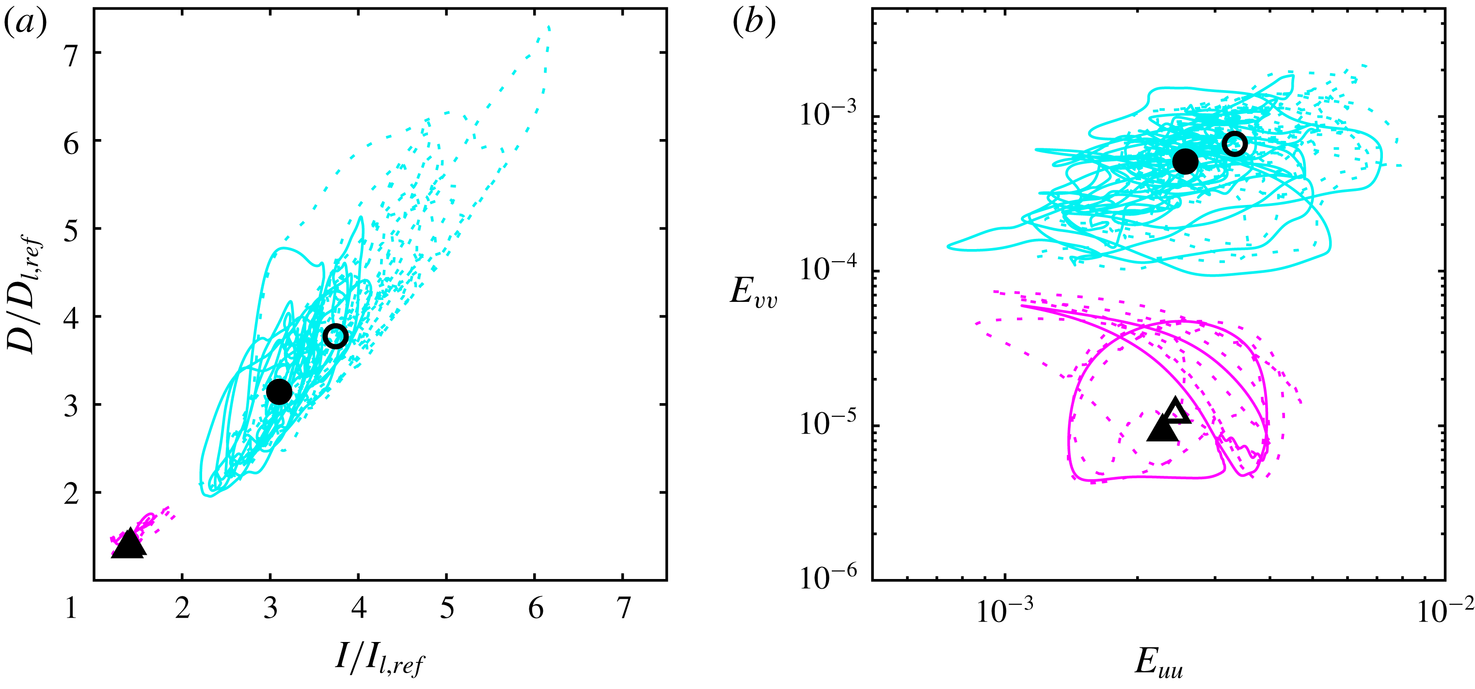
Figure 11 shows the $I$ – $D$ and $E_{uu}$ – $E_{vv}$ phase portraits of plane Poiseuille flow with and without control. The edge state, which consists of a periodic orbit in this case (see § 3.2), is plotted, along with its mean location in phase space. Again, we also plot the mean turbulent state and a typical turbulent trajectory. The change in behaviour of the system in $I$ – $D$ space when the control is applied (figure 11 a) is similar to that of Couette flow (see figure 10 a): the mean location of the edge state moves very slightly, but the mean turbulent state moves much closer to it. We also observe that the turbulent trajectory again occupies a smaller region of phase space and that the mean turbulent state is manipulated more than the edge state by the control in $E_{uu}$ – $E_{vv}$ phase space (figure 11 b). For the turbulent state in Poiseuille flow with $\unicode[STIX]{x1D719}=1.0$ , the r.m.s. fluctuations of $I$ and $D$ fall by 49 % and 39 %, respectively, when compared to the turbulent state with $\unicode[STIX]{x1D719}=0.0$ .

Figure 11.

Phase portrait of Poiseuille flow at $Re=4200$ with $\unicode[STIX]{x1D719}=0.0$ (dotted lines/open symbols) and $\unicode[STIX]{x1D719}=1.0$ (solid lines/closed symbols): (a)  $I/I_{l,ref}$ versus $D/D_{l,ref}$ , where $I_{l,ref}$ and $D_{l,ref}$ are the corresponding energy input and dissipation of the uncontrolled laminar flow at the same Reynolds number; (b)  $E_{uu}$ versus $E_{vv}$ . Here, cyan lines, fully developed simulations; magenta lines, edge state; circles, mean turbulent state; triangles, mean of the edge state.

As discussed above, the upper-branch equilibrium solution is an element forming the ‘skeleton’ of the turbulent trajectory in phase space. These equilibria are unstable by nature. In both plane Couette flow and Poiseuille flow, we see that not only does the mean turbulent state move closer to the edge state but also the fluctuations in $I$ and $D$ about this mean are noticeably reduced. This suggests that the stability of the upper-branch solution is also modified in some way by the control such that it may become less ‘repelling’ in phase space. In order to analyse this, we examine the eigenvalues of the equilibrium solutions, which are computed by Arnoldi iteration (see § 2.2.1). Figure 12 shows how the eigenvalues of the lower- and upper-branch solutions change when the control is applied. Firstly, as we would expect, the eigenvalues for the lower-branch solution (figure 12 a) are modified very little. In particular, the one unstable eigenvalue is not modified at all. For the upper-branch solution (figure 12 b), we see a much more significant change in the eigenvalues and the real part of the leading unstable eigenvalue is reduced by almost a half. This implies that the repelling strength of the upper-branch solution is indeed reduced by the control as the turbulent trajectory approaches it in phase space. Therefore, this would explain why we observe a significant reduction in $I$ and $D$ fluctuations in both Couette flow and Poiseuille flow for the $\unicode[STIX]{x1D719}=1.0$ case. The number of unstable eigenvalues with and without control could also be related to the reduction in $I$ and $D$ fluctuations of the turbulent state. Fewer unstable eigenvalues would imply fewer possible trajectories away from the upper-branch solution, which could also cause a reduction in the $I$ and $D$ fluctuations. For $\unicode[STIX]{x1D719}=0.0$ there is one real unstable eigenvalue and ten complex conjugate pairs of unstable eigenvalues for the upper-branch equilibrium solution, whereas for $\unicode[STIX]{x1D719}=1.0$ there are just ten complex conjugate pairs of unstable eigenvalues. Therefore, this is clearly only a weak effect. As a final point, in figure 13, we plot the change in the eigenvalues of the upper-branch solution without control as the Reynolds number is reduced from $Re=400$ to 300 and note that the leading unstable eigenvalues also reduce in magnitude. This similarity suggests that the control also somewhat regularises the behaviour of the turbulent trajectory in phase space as well as the edge state.

Figure 12.

Eigenspectra of equilibrium solutions of Couette flow at $Re=400$ with $\unicode[STIX]{x1D719}=0.0$ (open symbols) and $\unicode[STIX]{x1D719}=1.0$ (closed symbols): (a) lower-branch solution; (b) upper-branch solution. In each case, the 20 most unstable eigenvalues are shown.

Figure 13.

Eigenspectra of upper-branch equilibrium solution of Couette flow at $Re=400$ (open symbols) and $Re=300$ (closed symbols) with $\unicode[STIX]{x1D719}=0.0$ for comparison with figure 12. In each case, the 20 most unstable eigenvalues are shown.

3.3.2 Lifetime statistics of Couette and Poiseuille flow

Thus far, we have observed that the upper-branch equilibrium solution and mean turbulent state gradually approach the edge state as the control amplitude is increased. We note that this observation is made only with two simple state-space projections (i.e. the $I$ – $D$ and $E_{uu}$ – $E_{vv}$ phase spaces). Given the very high-dimensional nature of the present systems, these projections are evidently not ideal, and, as such, it may be possible to define a better, higher-dimensional state-space projection or relevant measure of the distance between two states. However, it should also be pointed out that the introduction of another state-space projection does not necessarily provide any new physical insight into the dynamics of the turbulent state, because the choice of any such projection would contain a certain degree of ‘arbitrariness’. For this reason, here, we aim to study the statistical features of turbulence that would be directly relevant to the physical implication of the reduced distance between the turbulent state and the edge of turbulence.

Since the edge of turbulence is not compact in phase space, the reduced distance in phase space between the turbulent state and the edge state observed in the previous sections indicates that opposition control may increase the probability of escaping from the turbulent state, which takes the form of a chaotic saddle. In other words, the control may increase the probability of laminarisation. Therefore, the final step in the present study is to assess how opposition control alters the turbulence lifetime statistics of Couette flow and Poiseuille flow, bearing in mind the change in their phase-space dynamics. We generate 100 different turbulent flow fields for both Couette flow and Poiseuille flow by running long simulations at a slightly elevated Reynolds number ( $Re=415$ for Couette flow and $Re=4350$ for Poiseuille flow) and then taking snapshots of the flow field at regular intervals. In each case, these 100 flow fields are used as initial conditions for a turbulence lifetime study at the nominal Reynolds numbers given in table 1. The temporal evolution of the initial conditions are tracked up to $t=5000h/U_{ref}$ for the five different control amplitudes $\unicode[STIX]{x1D719}=0.0,0.1,0.2,0.5$ and 1.0. We then determine the time it takes for each flow field to decay to the laminar solution (if at all) by defining a threshold of the cross-flow turbulent fluctuation energy below which turbulence cannot be recovered. In other words, the lifetime of a given initial condition is defined as the time taken for the flow to satisfy $(E_{vv}+E_{ww})<\unicode[STIX]{x1D716}$ . We choose $\unicode[STIX]{x1D716}=10^{-4}$ and $10^{-5}$ for Couette flow and Poiseuille flow, respectively. It is then possible to compute the probability of turbulence as a function of time for each value of $\unicode[STIX]{x1D719}$ . This is defined as the fraction of the 100 initial flow fields that remain turbulent at a given time instant up to $t=5000h/U_{ref}$ .

The results are plotted on semi-logarithmic axes in figure 14 for both flows. For the $\unicode[STIX]{x1D719}=0.0$ case in both Couette flow (figure 14 a) and Poiseuille flow (figure 14 b), we see an initial region that depends on the nature of the initial conditions, followed by an approximately exponential distribution that is characteristic of turbulence lifetimes (Eckhardt et al. Reference Eckhardt, Schneider, Hof and Westerweel2007). This verifies that the sample of 100 initial conditions used in this turbulence lifetimes study is sufficiently large and varied in each case. The first point to note is that the control has a very similar effect on the lifetime statistics of both flows: in general, as the control amplitude is increased, the probability of turbulence at a given time decreases. This change is small for lower amplitudes of control and more pronounced at $\unicode[STIX]{x1D719}=1.0$ . Interestingly, the effect of increasing the control amplitude is similar to the effect of decreasing the Reynolds number, indicating again that opposition control regularises the turbulent state as well as reducing its drag. It would seem, therefore, that this progressive decrease in turbulence lifetimes is related to the gradual approach of the upper-branch equilibrium solution and mean turbulent state towards the edge state in phase space as the control amplitude is increased.

Figure 14.

Probability of turbulence as a function of time for various control amplitudes: (a) Couette flow at $Re=400$ ; (b) Poiseuille flow at $Re=4200$ .

Figure 15.

Variation of (a) $\unicode[STIX]{x0394}D_{1}$ and (b)  $\unicode[STIX]{x0394}D_{2}$ with $\unicode[STIX]{x1D719}$ . Here, circles, Couette flow at $Re=400$ ; triangles, Poiseuille flow at $Re=4200$ : $\unicode[STIX]{x0394}D_{1}$ and $\unicode[STIX]{x0394}D_{2}$ are defined by (3.2a ) and (3.2b ), respectively.

At first glance, it might seem obvious that this would increase the likelihood of the turbulent trajectory passing through the edge state and decaying to the laminar solution. However, as discussed in § 3.3.1, the fluctuations of the turbulent state about its mean in the $I$ – $D$ plane seem also to be reduced by the control, which would actually reduce the probability of the solution passing through the edge state (or increase the probability of turbulence in time). Therefore, we further investigate this by calculating the distance between the turbulent trajectory and the edge state in terms of the dissipation, $D$ . We define two parameters:

(3.2a ) $$\begin{eqnarray}\unicode[STIX]{x0394}D_{1}=D_{mean}-D_{edge},\end{eqnarray}$$

where $D_{mean}$ is the mean dissipation of the turbulent state and $D_{edge}$ is the mean dissipation of the edge state, and

(3.2b ) $$\begin{eqnarray}\unicode[STIX]{x0394}D_{2}=(D_{mean}-D_{rms})-D_{edge},\end{eqnarray}$$

where $D_{rms}$ is the root mean squared fluctuation of the dissipation of the turbulent state. The expression (3.2a ) corresponds to the distance in $D$ space between the mean turbulent state and the edge state. As we have seen (figure 10 a; figure 11 a), this should decrease on increasing $\unicode[STIX]{x1D719}$ . By taking into account the magnitude of the fluctuations of the turbulent state about its mean, equation (3.2b ) is therefore a representation of the shortest possible distance in $D$ space between the edge state and the turbulent trajectory. This gives a more complete description of the actual proximity of the two states in phase space.

In figure 15, we show the variation in $\unicode[STIX]{x0394}D_{1}$ and $\unicode[STIX]{x0394}D_{2}$ with the control amplitude for Couette flow and Poiseuille flow. What we see is that both $\unicode[STIX]{x0394}D_{1}$ and $\unicode[STIX]{x0394}D_{2}$ decrease considerably as the control amplitude is increased. This verifies that not only does the turbulent trajectory reside closer to the edge state on average for larger $\unicode[STIX]{x1D719}$ , but also that the shortest distance between the two states is significantly reduced. This occurs despite the fluctuations being damped by the control and explains more precisely why the probability of turbulence decreases as the control amplitude increases.