1 Introduction
Nonlinear invariant solutions of the incompressible Navier–Stokes (NS) equations, such as equilibria (Nagata Reference Nagata1990) or periodic orbits (Kawahara & Kida Reference Kawahara and Kida2001), are believed to play an important role in transitional and self-sustaining turbulence. In particular, it has been proposed that coherent structures in turbulent flows are incomplete representations of such solutions, corresponding to times in which the flow approaches an invariant solution in phase space (Jiménez Reference Jiménez1987). The solutions themselves could then be considered ‘exact’ coherent structures (Waleffe Reference Waleffe2001). Their properties and significance are reviewed in Kawahara, Uhlmann & Van Veen (Reference Kawahara, Uhlmann and Van Veen2012).
An additional advantage of invariant solutions in the description of turbulence is that they can be exactly reproduced numerically, potentially providing a well-defined dynamical ‘alphabet’ for the flow evolution, and chaotic fluid motions are created by homoclinic or heteroclinic entanglement of their stable/unstable manifolds. Their statistical agreement with turbulence at low Reynolds numbers has often been noted in the literature (Kawahara & Kida Reference Kawahara and Kida2001; Jiménez et al. Reference Jiménez, Kawahara, Simens, Nagata and Shiba2005; Kerswell & Tutty Reference Kerswell and Tutty2007; Viswanath Reference Viswanath2007). Unfortunately, the dynamically important solutions embedded in turbulence have only been found at low Reynolds numbers in wall-bounded flows such as plane Poiseuille or Couette flow (Kawahara & Kida Reference Kawahara and Kida2001; van Veen & Kawahara Reference van Veen and Kawahara2011; Kreilos & Eckhardt Reference Kreilos and Eckhardt2012; Park & Graham Reference Park and Graham2015). From a practical point of view, they are hard to continue to higher Reynolds numbers partly because of their increasing complexity and instability, and by the limitations of the numerical resources. From the theoretical side, their increasing instability as the Reynolds number increases calls into question whether the flow would approach them often enough for them to be considered relevant. There has also been a challenge to estimate turbulence statistics by using all of recurrent flows (Chandler & Kerswell Reference Chandler and Kerswell2013; Cvitanović Reference Cvitanović2013); however, such an exhaustive study is still limited to low Reynolds numbers. A more promising method will be required to find invariant solutions at high Reynolds numbers with a large number of degrees of freedom, such as the multiple-shooting method (Sánchez & Net Reference Sánchez and Net2010; van Veen, Kawahara & Matsumura Reference van Veen, Kawahara and Matsumura2011). As a consequence they have mostly been discussed in the context of the transition to turbulence from the laminar state (Schmiegel & Eckhardt Reference Schmiegel and Eckhardt1997; Faisst & Eckhardt Reference Faisst and Eckhardt2003; Wedin & Kerswell Reference Wedin and Kerswell2004; Wang, Gibson & Waleffe Reference Wang, Gibson and Waleffe2007; Itano & Generalis Reference Itano and Generalis2009; Avila et al. Reference Avila, Mellibovsky, Roland and Hof2013; Zammert & Eckhardt Reference Zammert and Eckhardt2015).
The dynamical system approach to the transition to turbulence advocates that there is an edge state on the basin boundary between the linearly stable laminar state and turbulent state, which can be captured by edge tracking (Itano & Toh Reference Itano and Toh2001; Toh & Itano Reference Toh and Itano2003; Skufca, Yorke & Eckhardt Reference Skufca, Yorke and Eckhardt2006). Typically, it determines how the fluid behaves as it transitions from laminar to turbulent states and vice versa. Some of the lower-branch solutions often sit on the edge state, and form a critical layer at high Reynolds number (Wang et al. Reference Wang, Gibson and Waleffe2007; Viswanath Reference Viswanath2009). Such critical-layer-type solutions are described by an asymptotic theory called vortex–wave interaction (VWI) (Hall & Smith Reference Hall and Smith1991; Hall & Sherwin Reference Hall and Sherwin2010) and their instability has the edge mode (Deguchi & Hall Reference Deguchi and Hall2016). It is shown that vertically localised equilibrium states can be embedded in any shear flow at high Reynolds number (Blackburn, Hall & Sherwin Reference Blackburn, Hall and Sherwin2013; Deguchi & Hall Reference Deguchi and Hall2014a ; Deguchi Reference Deguchi2015).
The multiscale nature of fully developed turbulence at high Reynolds number and the possible role of coherent structures in the energy cascade raise the question of whether invariant solutions may also be relevant in such processes. Van Veen, Kida & Kawahara (Reference van Veen, Kida and Kawahara2006) found a periodic orbit in highly symmetric turbulence that results in a
 $k^{-5/3}$
energy spectrum, and could be part of the generic energy cascade (Goto Reference Goto2008). Similar attempts, however, have not been successful in wall-bounded turbulence at high Reynolds number, because it is difficult to accommodate the anisotropy and inhomogeneity of the length scales introduced by the wall.
Here, we simplify the problem in two ways. In the first place we substitute shear-driven wall-bounded flow by a homogeneous shear without walls, the large-scale motion of which is limited by the spanwise box dimension in a long-term simulation (Sekimoto, Dong & Jiménez Reference Sekimoto, Dong and Jiménez2016). Secondly, we substitute the full NS equations by large-eddy simulations (LES), the small-scale property of which is determined by the eddy viscosity.
Homogeneous shear turbulence is an idealised case that shares with wall-bounded flows the basic source of turbulent energy by the shear. Ideal unbounded homogeneous shear flow has no intrinsic length scale and is believed to grow without bound from any initial condition (Champagne, Harris & Corrsin Reference Champagne, Harris and Corrsin1970; Rogers & Moin Reference Rogers and Moin1987; Tavoularis & Karnik Reference Tavoularis and Karnik1989; Cambon & Scott Reference Cambon and Scott1999) but, when simulated in a finite computational box, it reaches a statistically stationary and homogeneous state (SS-HST) characterised by repeated bursting reminiscent of near-wall and logarithmic-layer turbulence (Pumir Reference Pumir1996; Gualtieri et al. Reference Gualtieri, Casciola, Benzi and Piva2007). The problem was recently revisited by Sekimoto et al. (Reference Sekimoto, Dong and Jiménez2016) using direct numerical simulations (DNS), from which the simulation code and parameters in this paper are derived. They determined which computational boxes best mimic wall-bounded turbulence, and showed that the relevant limiting dimension is the spanwise box width. In terms of this dimension, SS-HST is always minimal in the sense that a single velocity streak tends to fill the whole span, as in minimal channels (Jiménez & Moin Reference Jiménez and Moin1991; Flores & Jiménez Reference Flores and Jiménez2010). They showed that this minimal flow, even with no walls, is a very promising model for shear turbulence with a non-inflectional mean profile, and particularly for the logarithmic layer of wall-bounded flows.
LES is based on the idea that the large flow scales, which are explicitly computed, are essentially independent of the smaller ones, which are typically modelled by some kind of eddy viscosity (Pope Reference Pope2000). In shear flows, the larger scales usually account for most of the kinetic energy and momentum transfer, while the smaller ones tend to be isotropic and basically provide dissipation and act as random perturbations. In particular, it is known that the large-scale motion is maintained in channels even when the small scales have been filtered in LES (Scovazzi, Jiménez & Moin Reference Scovazzi, Jiménez and Moin2001; Hwang & Cossu Reference Hwang and Cossu2010). The key idea of extending the dynamical system approach to higher Reynolds numbers is to focus on the quasi-autonomous behaviour of the larger scales by modelling the effect of the smaller ones using a subgrid (SG) model (Yasuda, Goto & Kawahara Reference Yasuda, Goto and Kawahara2014; Rawat et al. Reference Rawat, Cossu, Hwang and Rincon2015; Hwang, Willis & Cossu Reference Hwang, Willis and Cossu2016; Sasaki et al. Reference Sasaki, Kawahara, Sekimoto and Jiménez2016), where some LES steady states and periodic orbits are numerically obtained in wall-bounded flow and they are considered as a representation of large-scale motions. However, as mentioned above, the anisotropy and inhomogeneity of the length scales introduced by the wall makes the role of the eddy-viscosity term, which should be zero on the wall, on the invariant solutions ambiguous. We apply LES here to the identification of equilibrium structures in SS-HST, where the large length scale is constrained and represented by the spanwise box dimension and the smallest scale is imposed by an SG model, so that the scale separation is statistically homogeneous, and the length-scale ratio is used as a grid-independent LES parameter. The application of LES greatly also decreases the number of degrees of freedom required to track invariant solutions at high Reynolds number.
Section 2 presents the numerical method and establishes a baseline LES with sinuous (streamwise-shift-reflection and spanwise-shift-rotation) symmetry. Equilibria are numerically obtained and overviewed in § 3, focusing on lower-branch solutions. The dependences of the lower- and upper-branch equilibria on the computational domain and on the LES parameters are investigated in § 4, while §§ 4.2 and 4.3 discuss the vertical localisation of the equilibrium solutions and of the baseline LES. Finally, § 5 offers conclusions and future perspectives. An appendix discusses the linear stability of the equilibrium solutions.
2 Numerical methods
2.1 The governing equations
We solve the incompressible LES momentum and continuity equations,
 $$\begin{eqnarray}\displaystyle & \unicode[STIX]{x2202}_{t}\overline{u}_{i}+\overline{u}_{j}\unicode[STIX]{x2202}_{j}\overline{u}_{i}=-\unicode[STIX]{x2202}_{i}\overline{p}+\unicode[STIX]{x2202}_{j}(2\unicode[STIX]{x1D708}_{t}\overline{\unicode[STIX]{x1D70E}}_{ij}), & \displaystyle\end{eqnarray}$$
 $$\begin{eqnarray}\displaystyle & \unicode[STIX]{x2202}_{j}\overline{u}_{j}=0, & \displaystyle\end{eqnarray}$$
where
 $\overline{u}_{i}$
are the resolved (large-scale) velocities, and
 $\overline{p}$
is a modified resolved kinematic pressure that includes the diagonal part of the SG stress tensor. The eddy viscosity is written as
 $\unicode[STIX]{x1D708}_{t}=l_{S}^{2}|\overline{\unicode[STIX]{x1D70E}}|$
, in terms of a static length scale
 $l_{S}$
and of the local resolved strain rate (Smagorinsky Reference Smagorinsky1963), where
 $|\overline{\unicode[STIX]{x1D70E}}|^{2}=2\overline{\unicode[STIX]{x1D70E}}_{ij}\overline{\unicode[STIX]{x1D70E}}_{ij}$
and
 $\overline{\unicode[STIX]{x1D70E}}_{ij}=(\unicode[STIX]{x2202}_{j}\overline{u}_{i}+\unicode[STIX]{x2202}_{i}\overline{u}_{j})/2$
is the strain-rate tensor of the filtered velocity. We use
 $(x,y,z)$
to represent the streamwise, vertical (cross-shear) and spanwise coordinates, respectively, and
 $(u,v,w)$
to denote the respective velocity components. Whenever convenient, as in (2.1), this notation is substituted by subindices, in which case repeated indices imply summation. This is always the case for the vorticity components
 $\overline{\unicode[STIX]{x1D714}}_{i}$
. There is no explicit filtering in our code, and the smallest flow scales are controlled either by the grid or by the eddy viscosity.
It is usual in most LES to include the molecular viscosity
 $\unicode[STIX]{x1D708}$
as part of the right-hand side of (2.1), and to write the length
 $l_{S}$
in terms of some convenient grid spacing
 $\unicode[STIX]{x1D6E5}_{g}$
and of a ‘universal’ Smagorinsky constant
 $C_{S}$
. None of those devices are needed here, and will not be used. The main role of the molecular viscosity in LES is to enforce the boundary conditions when
 $\unicode[STIX]{x1D708}_{t}$
vanishes at the wall. Since there are no walls in our problem, we set
 $\unicode[STIX]{x1D708}=0$
, and all our simulations run at infinite molecular Reynolds number.
Similarly, the role of
 $\unicode[STIX]{x1D6E5}_{g}$
in SG models is to accommodate variable grid spacings, assuming that most of the spectral content of the velocity gradients is concentrated at the grid scale. Again, the statistical homogeneity of the flow implies that our grids are uniform, and makes this complication unnecessary.
In fact, the essential role of the eddy viscosity is to introduce a minimum length scale that takes the role of the Kolmogorov length,
 $\unicode[STIX]{x1D702}$
, independently of the grid. If we estimate the energy dissipation by the SG model as
 $\unicode[STIX]{x1D700}=\langle \unicode[STIX]{x1D708}_{t}|\overline{\unicode[STIX]{x1D70E}}|^{2}\rangle =l_{S}^{2}\langle |\overline{\unicode[STIX]{x1D70E}}|^{3}\rangle$
, and define an effective Kolmogorov length as
 $\unicode[STIX]{x1D702}_{t}=(\langle \unicode[STIX]{x1D708}_{t}\rangle ^{3}/\unicode[STIX]{x1D700})^{1/4}$
, it follows from the definition of
 $\unicode[STIX]{x1D708}_{t}$
that
 $\unicode[STIX]{x1D702}_{t}\approx l_{S}$
. Here
 $\langle \cdot \rangle$
represents time and space average, and will occasionally be replaced by
 $\langle \cdot \rangle _{xz}$
to represent the
 $y$
-dependent average over horizontal planes, or by
 $\langle \cdot \rangle _{c}$
to represent
 $\langle \cdot \rangle _{xz}$
particularised to the central plane
 $y=0$
. From now on, capital letters are reserved for mean quantities and lower-case ones for fluctuations with respect to that mean, as in
 $U=\langle \overline{u}\rangle _{xz}$
and
 $\overline{u}=U+u$
. Primes denote root-mean-squared (r.m.s.) intensities of the fluctuations.
Since most of the computational effort in DNS is dedicated to resolving the smallest dissipative scales, the introduction of a cut-off length in LES drastically reduces the size of the linear systems that have to be solved to obtain invariant solutions.
For the parallel flows that are the subject of this paper, (2.1) can be integrated to
 $$\begin{eqnarray}\displaystyle & \langle -uv+2\unicode[STIX]{x1D708}_{t}\overline{\unicode[STIX]{x1D70E}}_{xy}\rangle _{xz}=u_{\unicode[STIX]{x1D70F}}^{2}, & \displaystyle\end{eqnarray}$$
where
 $u_{\unicode[STIX]{x1D70F}}$
is independent of
 $y$
and can be used to scale the velocities. Variables in this scaling are denoted by a ‘+’ superscript.
2.2 LES with sinuous symmetry
We study a flow with a nominally uniform mean shear
 $S=\text{d}U/\text{d}y$
, which is a given constant, in a parallelepiped-shaped computational domain that is periodic in the
 $(x,z)$
directions, and periodic between points of the lower and upper boundaries that are uniformly shifted in time by the shear (Gerz, Schumann & Elghobashi Reference Gerz, Schumann and Elghobashi1989). The mean flow for turbulence statistics is
 $Sy$
plus the vertically periodic correction, which is an approximately linear profile as evaluated later in this section. The numerical code for DNS is described in detail in Sekimoto et al. (Reference Sekimoto, Dong and Jiménez2016). Equations (2.1) and (2.2) for LES are formulated in terms of the Sekimoto et al. (Reference Sekimoto, Dong and Jiménez2016). Equations (2.1) and (2.2) for LES are formulated in terms of the vertical vorticity and of the Laplacian of the vertical velocity (Kim, Moin & Moser Reference Kim, Moin and Moser.1987; Hughes, Oberai & Mazzei Reference Hughes, Oberai and Mazzei2001). The discretisation uses
 $2/3$
-dealiased Fourier expansions in
 $(x,z)$
, and sixth-order spectral-like compact finite differences in
 $y$
, with the shear-periodic boundary conditions embedded in the compact finite-difference matrices for each Fourier mode. As explained in Sekimoto et al. (Reference Sekimoto, Dong and Jiménez2016), this avoids recurrent remeshing and the resulting secular loss of enstrophy over long integration times.
There are three dimensionless parameters: a Reynolds number, and two box aspect ratios,
 $A_{xz}=L_{x}/L_{z}$
and
 $A_{yz}=L_{y}/L_{z}$
, where the
 $L_{j}$
are the dimensions of the computational domain along the three coordinate directions. It was shown in Sekimoto et al. (Reference Sekimoto, Dong and Jiménez2016) that the correct scales for the large-scale length and velocity of SS-HST are based on the spanwise box dimension,
 $L_{z}$
and
 $SL_{z}$
, so that the Reynolds number is
 $Re_{z}\equiv SL_{z}^{2}/\unicode[STIX]{x1D708}$
in DNS. We will extend this definition to LES using the effective mean eddy viscosity,
 $\langle \unicode[STIX]{x1D708}_{t}\rangle$
, replacing the molecular viscosity
 $\unicode[STIX]{x1D708}$
. However, it is more convenient to use the length-scale ratio
 $R_{S}=L_{z}/l_{S}$
in LES. For example, Piomelli, Rouhi & Geurts (Reference Piomelli, Rouhi and Geurts2015) recently developed a grid-independent LES using as parameter the ratio of the small (effective Kolmogorov) and integral scales, which is essentially the inverse of
 $R_{S}$
. It can be extended to DNS by substituting
 $\unicode[STIX]{x1D702}$
for
 $l_{S}$
(
 $L_{z}/\unicode[STIX]{x1D702}\sim Re_{z}^{3/4}$
) and it turns out that, in DNS of SS-HST,
 $Re_{z}\approx 4R_{S}^{4/3}$
(Sekimoto et al.
Reference Sekimoto, Dong and Jiménez2016). We will also use the integral scale
 $L_{0}=u_{0}^{3}/\unicode[STIX]{x1D700}$
, where
 $u_{0}^{2}=\langle u_{i}u_{i}\rangle /3$
.
We study in this paper LES turbulence and invariant solutions in a subspace defined by enforcing two ‘sinuous’ symmetries: (I) a reflection with respect to the plane of
 $z=0$
followed by a streamwise shift by
 $L_{x}/2$
,
 $$\begin{eqnarray}(\text{I}):\quad [u,v,w](x,y,z)=[u,v,-w](x+L_{x}/2,y,-z);\end{eqnarray}$$
and (II) a rotation by
 $\unicode[STIX]{x03C0}$
around
 $x=y=0$
followed by a spanwise shift by
 $L_{z}/2$
,
 $$\begin{eqnarray}(\text{II}):\quad [u,v,w](x,y,z)=[-u,-v,w](-x,-y,z+L_{z}/2).\end{eqnarray}$$
Note that no translational symmetries are allowed in this subspace, so that travelling waves are excluded. Moreover,
 $(\text{I})$
and
 $(\text{II})$
together with the boundary conditions enforce that the instantaneous plane-averaged streamwise velocities at the top and bottom of the box are
 $U(\pm L_{y}/2)=\pm SL_{y}/2$
.
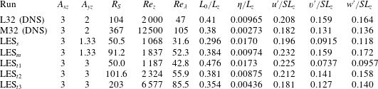
Before proceeding to seek equilibrium solutions, the effect of the symmetry restriction was tested in several LES of symmetric SS-HST, which are summarised in table 1. Table 1 also includes two reference unconstrained DNS from Sekimoto et al. (Reference Sekimoto, Dong and Jiménez2016), and shows that the length and velocity scales found in DNS also work well in the symmetric LES. Although not included in table 1, the effective Kolmogorov scale in the LES is found to be
 $\unicode[STIX]{x1D702}_{t}/l_{S}\approx 0.9$
, in approximate agreement with our analysis in § 2.1. Interestingly, both
 $\unicode[STIX]{x1D702}_{t}/l_{S}\approx 0.9$
–1.0 and
 $L_{0}/L_{z}\approx 0.4$
–0.7 remain good approximations in the localised equilibrium solutions described below. Note that the vertical translational invariance is broken by the symmetries (2.4) and (2.5), so that a uniform mean shear is no longer guaranteed. Even so, the LES of symmetric turbulence retain an approximately linear mean profile
 $(|U-Sy|\approx 0.01SL_{z})$
and approximately constant fluctuation profiles. We will see below that the same is not generally true for the profiles of the equilibrium solutions.
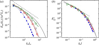
Figure 1 displays the longitudinal streamwise-velocity spectrum of the symmetric LES turbulence, compared to that of the reference DNS. Given the different Reynolds numbers and techniques, the agreement is good, showing that symmetry does not influence turbulence greatly. Note that the three LES in figure 1(b) collapse well in terms of
 $l_{S}$
, and that the resolution of the simulations is fine enough to resolve the smallest LES scales.
Parameters for the turbulence runs. L32 and M32 are reference DNS of SS-HST from Sekimoto et al. (Reference Sekimoto, Dong and Jiménez2016). LES
 $_{s,m,t1,t2,t3}$
are the present LES in the symmetric subspace defined by (I)
 $+$
(II) in (2.4) and (2.5). The effective Reynolds number,
 $Re_{z}$
, and the Kolmogorov viscous scale,
 $\unicode[STIX]{x1D702}$
, are computed with the molecular viscosity in DNS, and with the averaged eddy viscosity in LES. The scale ratio
 $R_{S}$
is
 $L_{z}/l_{S}$
in LES and
 $L_{z}/\unicode[STIX]{x1D702}$
in DNS. The Reynolds number
 $Re_{\unicode[STIX]{x1D706}}\equiv u_{0}\unicode[STIX]{x1D706}/\langle \unicode[STIX]{x1D708}_{t}\rangle$
is that based on the Taylor microscale
 $\unicode[STIX]{x1D706}=\sqrt{15}u_{0}/\langle \unicode[STIX]{x1D714}_{i}\unicode[STIX]{x1D714}_{i}\rangle ^{1/2}$
.

Streamwise velocity spectra
 $E_{uu}(k_{x})$
. (a) Large-scale normalisation,
 $E_{uu}/(u^{\prime 2}L_{z})$
, as a function of
 $k_{x}L_{z}$
. (b) Small-scale normalisation,
 $E_{uu}^{\ast }\equiv \unicode[STIX]{x1D700}^{-2/3}l^{-5/3}E_{uu}(k_{x}l)$
, with
 $l=l_{S}$
for LES and
 $l=\unicode[STIX]{x1D702}$
for DNS. Curves/symbols: – –
 $\triangledown$
– – (grey), DNS (L32); —— (grey), DNS (M32); – –
 $\bullet$
– – (blue),
 $R_{S}=52.6$
; —
 $\circ$
— (red),
 $R_{S}=101.6$
; —
 $\rhd$
— (green),
 $R_{S}=203$
. The slope of the chain-dotted diagonal is
 $-5/3$
.

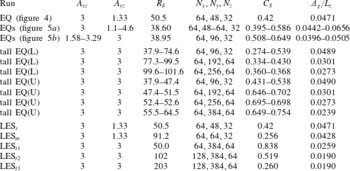
The size of the collocation grids for the turbulence LES and for typical equilibrium solutions are given in table 2. It follows from the definition of the different quantities that the collocation resolution is
 $\unicode[STIX]{x0394}x/l_{S}=R_{S}A_{xz}/N_{x}$
,
 $\unicode[STIX]{x0394}y/l_{S}=R_{S}A_{yz}/N_{y}$
and
 $\unicode[STIX]{x0394}z/l_{S}=R_{S}/N_{z}$
, where the
 $N_{j}$
are the collocation points along the three coordinate directions. For example, in the lowest-Reynolds-number LES
 $_{s}$
in tables 1 and 2, this results in
 $(\unicode[STIX]{x0394}x,\unicode[STIX]{x0394}y,\unicode[STIX]{x0394}z)=(3.6,1.4,2.7)l_{S}$
. If our SG model is interpreted in terms of the usual Smagorinsky formula
 $\unicode[STIX]{x1D708}_{t}=(C_{S}\unicode[STIX]{x1D6E5})^{2}|\overline{\unicode[STIX]{x1D70E}}|$
, with
 $\unicode[STIX]{x1D6E5}$
a representative grid spacing, it follows that
 $C_{S}=l_{S}/\unicode[STIX]{x1D6E5}=0.42$
, which is a relatively high value for usual LES practice. In this sense, all our LES are overdamped. Their dynamics are controlled not by the grid, but by the SG model, and can be expected to be approximately independent of the resolution. They also only resolved the integral scales of the flow, and very little of its inertial range. The effective Smagorinsky constant for the different simulations is included in table 2.
Grid information for the sinuous-symmetric equilibrium and turbulence LES. EQ(L) and EQ(U) represent lower- and upper-branch equilibrium solutions, respectively, and the turbulence LES are defined in table 1. The effective Smagorinsky constant
 $C_{S}$
is discussed in § 2.2, with the filter scale defined as
 $\unicode[STIX]{x1D6E5}_{g}\equiv \sqrt[3]{\unicode[STIX]{x0394}x\unicode[STIX]{x0394}y\unicode[STIX]{x0394}z}$
.

At box aspect ratios
 $(A_{xz},A_{yz})=(3,1.33)$
, symmetric self-sustaining LES turbulence exists for
 $R_{S}\gtrsim 65$
. There is a transitional range,
 $45\lesssim R_{S}\lesssim 65$
, in which the kinetic energy of the flow increases and decreases several times before decaying to laminar after
 $St=O(1000)$
. Both the transitional range and the decay time depend somewhat on
 $A_{yz}$
. We will see in § 4 that LES turbulence in taller boxes,
 $A_{yz}\approx 2$
–3, survives in the range
 $50\lesssim R_{S}\lesssim 60$
, but collapses intermittently to vertically localised turbulence.
2.3 Searching for invariant solutions in LES
Our main interest is to characterise invariant solutions in LES of SS-HST. Strictly equilibrium solutions are technically impossible in this system. The shear-periodic boundary condition slides the upper computational boundary with a velocity
 $SL_{y}$
with respect to the lower one, and the numerical configuration only repeats itself after a ‘box’ period
 $T_{s}\equiv L_{x}/(SL_{y})$
. It was shown in Sekimoto et al. (Reference Sekimoto, Dong and Jiménez2016) that this periodic forcing does not interfere strongly with the turbulent solutions as long as the aspect ratios are kept in the range
 $2<A_{xz}\lesssim 5$
and
 $A_{xz}\lesssim 2A_{yz}$
. We will approximately respect these constraints here, and find solutions that are numerically indistinguishable from fixed points. Vertically localised solutions can be equilibria at the limit of
 $A_{yz}\rightarrow \infty$
, since they are independent of the shear-periodic boundary condition, but it should be remembered that all of them are conceptually periodic orbits in a finite computational domain. All of the statistics discussed below are averages over a box period.
Solutions are computed using the Newton–Krylov–hookstep method (Viswanath Reference Viswanath2007) on
 $\boldsymbol{f}^{T}(\boldsymbol{x})-\boldsymbol{x}=0$
, where
 $\boldsymbol{x}$
is the vector of independent variables, and
 $\boldsymbol{f}^{T}:\boldsymbol{x}(0)\rightarrow \boldsymbol{x}(T)$
is the integration of (2.1) over time
 $T$
, using the evolution code described in the previous section. Because of the periodicity mentioned above, the search time is always an integer multiple of the box period,
 $T_{m}=mT_{s}$
. The convergence criterion for the relative error of the Newton method is generally taken as
 $\Vert \boldsymbol{f}^{T_{m}}(\boldsymbol{x})-\boldsymbol{x}\Vert /\Vert \boldsymbol{x}\Vert <10^{-5}$
, where
 $\Vert \cdot \Vert$
is the
 $L_{2}$
norm.
The initial condition for the search was taken from snapshots of the LES symmetric turbulence in the above-mentioned marginal range in which turbulence eventually decays to laminar,
 $R_{S}<50$
,
 $A_{xz}=3$
and
 $A_{yz}=1.33$
. In order to find a solution, we fix the aspect ratios and the time period
 $T_{m}\approx 10$
(
 $m=5$
), then change
 $R_{S}$
. For
 $R_{S}\approx 35$
, the Newton search always converges to a trivial laminar state. The first non-trivial solution is obtained spontaneously at
 $R_{S}=38.6$
, and a trial with
 $m=7$
converges to the same solution. It is, therefore, a periodic orbit with the period of
 $T_{m}=T_{s}$
(
 $m=1$
) close to the bifurcation point that marks the lowest
 $R_{S}$
of our family of solutions. The solutions are always unstable and some examples of the linear stability analysis are shown in the later section and in the Appendix.
From this initial solution, lower and upper branches are continued along the parameters
 $A_{xz},~A_{yz}$
and
 $R_{S}$
, overcoming the turning points with a pseudo-arclength method. We have seen that all these solutions are periodic orbits in which the period is
 $T_{s}$
. The periodicity is especially noticeable for the upper-branch solutions in flat boxes,
 $A_{yz}=1.33$
–1.64 and
 $R_{S}\approx 45$
, where the temporal oscillation of the integrated kinetic energy is of order 1 %. They asymptotically approach a fixed point in the limit of
 $A_{yz}\rightarrow \infty$
, and the oscillations become negligible,
 $O(10^{-5})$
for
 $A_{yz}>2$
, for the vertically localised solutions described later in taller boxes.
3 Lower-branch solutions in LES
Here, we preview the obtained equilibria, and characterise lower-branch solutions in a computational box,
 $(A_{xz},A_{yz})=(3,1.33)$
. This is slightly ‘flatter’ than the acceptable range,
 $A_{xz}\lesssim 2A_{yz}$
, in which unphysical strong linear bursts appear as described in Sekimoto et al. (Reference Sekimoto, Dong and Jiménez2016), in spite of which the turbulence statistics are reasonably close to the logarithmic layer of channel turbulence. We investigate in this section the
 $R_{S}$
dependence of the equilibria. The effect of the aspect ratios is discussed in § 4.1.
All the equilibria in this section are found using the same numerical grid of the low-
 $R_{S}$
turbulence LES
 $_{s}$
in table 2,
 $(N_{x},N_{y},N_{z})=(64,48,32)$
. They are continued in
 $R_{S}$
as long as convergence is achieved. This happens in
 $R_{S}\lesssim 100$
for the lower-branch solutions, and in
 $R_{S}\lesssim 60$
for the upper branch. We emphasise that
 $R_{S}$
depends on the eddy-viscosity parameter
 $l_{S}$
, rather than on the numerical grid. As long as the numerics resolves features of the order of
 $\unicode[STIX]{x1D702}_{t}\approx l_{S}$
, all grids should converge to the same solution. We saw in the previous section that this is true for most of our simulations. As a further check, finer grids are used in § 4 to compute equilibria in other numerical boxes. In the cases in which the same solution is computed with two different grids, no substantial differences are found (see figure 5).
Although most solutions were converged to a Newton relative error of
 $10^{-5}$
, a few were confirmed to a tighter tolerance. For example, the lower- and upper-branch solutions at
 $R_{S}=50.5$
discussed in figures 3 and 4 are iterated to an accuracy of
 $10^{-12}$
.
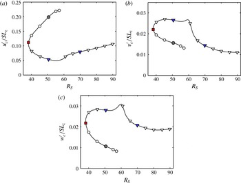
Figure 2(a–c) shows continuation diagrams of the lower- and upper-branch solutions for the box mentioned above, showing the fluctuation intensity of the three velocity components at
 $y=0$
. The lower-branch solutions are characterised by weaker streamwise velocity fluctuations and stronger transverse velocities than those in the upper branch, but note that even the more intense transverse velocity fluctuations,
 $v^{\prime }$
and
 $w^{\prime }$
, are an order of magnitude smaller than in the LES and DNS turbulence at a comparable Reynolds number in table 1
 $(v^{\prime }\approx w^{\prime }\approx 0.16SL_{z})$
.
(a–c) Velocity fluctuation intensities at the centre plane
 $y=0$
, as functions of
 $R_{S}=L_{z}/l_{S}$
, for
 $(A_{xz},A_{yz})=(3,1.33)$
: (a) streamwise component,
 $u_{c}^{\prime }$
; (b) vertical,
 $v_{c}^{\prime }$
; and (c) spanwise
 $w_{c}^{\prime }$
. Symbols: (
 $\circ$
, black) the upper branch; (
 $\triangledown$
, blue) the lower branch; solid symbols are cases plotted in figure 3.

Vortical structures and the velocity streaks in a box
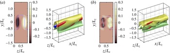
 $(A_{xz},A_{yz})=(3,1.33)$
: (a)
 $R_{S}=50.5$
, upper branch; (b)
 $R_{S}=38.2$
at the bifurcation point; (c)
 $R_{S}=50.5$
, lower branch; (d)
 $R_{S}=69.8$
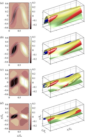
, lower branch. The shaded backgrounds in the left panels are isocontours of the streamwise-averaged
 $\unicode[STIX]{x1D714}_{x}(y,z)/S=[-0.3:0.03:0.3]$
. The light-grey dashed line is the streamwise-averaged
 $\overline{u}=0$
. The right panels shows the isosurfaces of
 $\unicode[STIX]{x1D714}_{x}=0.6|\unicode[STIX]{x1D714}_{x}|_{max}$
(red; dark-grey in black/white),
 $\unicode[STIX]{x1D714}_{x}=-0.6|\unicode[STIX]{x1D714}_{x}|_{max}$
(blue; black) and
 $\overline{u}=0$
(yellow; light-grey), gradually coloured by
 $y$
.

LES equilibrium solutions,
 $(A_{xz},A_{yz})=(3,1.33)$
and
 $R_{S}=50.5$
. (a) Mean streamwise velocity. The thin diagonal is
 $U=Sy$
. (b) Resolved strain rate. In (a,b): ——, lower branch, as in figure 3(a); - - - -, upper branch, as in figure 3(c). (c) Stability eigenvalues
 $(\unicode[STIX]{x1D707}_{r}+\text{i}\unicode[STIX]{x1D707}_{i})/S$
of the equilibria in (a,b):
 $\triangledown$
(blue), lower branch;
 $\circ$
(red), upper branch. (d) Temporal evolution of the fluctuation velocity magnitude of symmetric LES initialised from the equilibria in (a,b). The darker lines are initialised without any disturbance except numerical inaccuracies: —— (dark blue), initialised from the lower branch; - - - - (dark red), from the upper branch. The lighter grey lines are initialised from the lower branch with a small disturbance along the unstable direction corresponding to the real unstable mode: ——, attracted to the turbulence state; - - - -, attracted to the laminar state. All attempts to perturb the upper branch along its unstable modes led to laminarisation. The short thick dotted line represents the fluctuation intensity of LES
 $_{s}$
in table 1, using the same box and Reynolds number.

The identification of which branch is the lower one is not straightforward, but we will denote as such the lower branch in figure 2(a). This is actually consistent with the fact that the lower-branch solution typically has low drag, while the upper one has high drag (figure 6
c), as we shall discuss later in § 4.1. Continuation in
 $R_{S}$
reveals that, as this branch extends towards higher
 $R_{S}$
, its solutions concentrate in a relatively thin critical layer for
 $R_{S}>70$
. This is a common feature of lower-branch solutions in wall-bounded flows at high Reynolds numbers (Wang et al.
Reference Wang, Gibson and Waleffe2007; Viswanath Reference Viswanath2009; Hall & Sherwin Reference Hall and Sherwin2010; Blackburn et al.
Reference Blackburn, Hall and Sherwin2013; Deguchi, Hall & Walton Reference Deguchi, Hall and Walton2013). Figure 3 shows isosurfaces of
 $|\unicode[STIX]{x1D714}_{x}|=0.6|\unicode[STIX]{x1D714}_{x}|_{max}$
, and of
 $\overline{u}=0$
, representing the geometry of the vortical structures and of the velocity streak in the upper- and lower-branch solutions, showing that they are localised around
 $y=0$
. The streamwise-velocity streak of the lower-branch solutions meanders more deeply than the one in the upper branch, leading to stronger cross-flow velocity fluctuations. As
 $R_{S}$
increases, the vortical structure of lower-branch solutions becomes flatter. This occurs drastically, but smoothly, at around
 $R_{S}\approx 60$
, after which it becomes a critical-layer-type solution similar to those described by the VWI theory for the lower-branch solutions in plane Couette flow (Blackburn et al.
Reference Blackburn, Hall and Sherwin2013). This transition probably corresponds to a complex set of bifurcations, since several eigenvalues change stability around that
 $R_{S}$
, but tracking them is difficult in our flow. For example, a new complex pair appears around
 $R_{S}=55$
, but the associated branch cannot be followed by the present method because its period is not a simple multiple of the box period
 $T_{s}$
.
In the high-Reynolds-number limit, Blackburn et al. (Reference Blackburn, Hall and Sherwin2013) have shown that the VWI states begin to localise at
 $y=0$
as spanwise wavenumbers increase, i.e. as
 $L_{z}$
narrows. Waleffe (Reference Waleffe1997) showed that equilibrium solutions similar to those of Couette flow are generic to many shear flows, and Deguchi & Hall (Reference Deguchi and Hall2014a
) and Deguchi (Reference Deguchi2015) have described more recently how a VWI state can be embedded in any shear flow at high Reynolds number. There is an inviscid mechanism as in VWI-type solutions of the Navier–Stokes equation, whose streamwise velocity structure is shown to be thinner for increasing
 $Re$
. ‘The singularity occurs where the wave propagates downstream with the local fluid velocity and defines the location of a critical layer in which viscosity smooths out the singularity’ (Deguchi & Hall Reference Deguchi and Hall2016). The critical layers in LES equilibria must be similar to those in DNS and the singularity occurs, but the eddy viscosity smooths it out.
Upper-branch solutions are characterised by their taller streamwise-velocity streaks. Their height increases with increasing
 $R_{S}$
, while their quasi-streamwise vortices become more inclined (see figure 3
a). The relatively tall streaks suggest that the effect of the vertical box aspect ratio may be important for these solutions. This will be investigated in the next section.
Mean profiles for upper- and lower-branch solutions at the same
 $R_{S}$
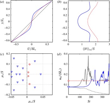
are shown in figure 4(a,b). The lower-branch solution is the one shown in figure 3(c), and the upper-branch one is in figure 3(a). Both solutions are concentrated around
 $y=0$
, but the concentration is more pronounced in the lower branch. This is seen in the more horizontal quasi-streamwise rollers in figure 3(c), and in the shallower mean velocity profile near
 $y=0$
in figure 4(a).
Since it follows from the momentum conservation equation (2.3) that the total shear stress has to be independent of
 $y$
, the shallower profile of the lower branch suggests a higher eddy viscosity, and consequently a higher total strain. The opposite turns out to be the case. Figure 4(b) displays the mean profile of the mean total strain rate for the two solutions, which can also be interpreted as a profile of eddy viscosity. The flatter profile of the lower branch is due to higher resolved Reynolds stresses. Beyond
 $|y|/L_{z}\approx 0.5$
, the mean strain tends to
 $\langle |\overline{\unicode[STIX]{x1D70E}}|\rangle _{xz}\approx \text{d}U/\text{d}y$
, and most of the momentum flux is carried by the SG term.
The simplest interpretation is that the Reynolds stresses created by the transverse velocities of the equilibrium state flatten the profile into a local region of lower shear. This results in a locally lower eddy viscosity and a locally higher Reynolds number, which helps to sustain the solution. However, the requirement from the boundary condition that the total velocity difference across the domain is constant prevents the low-shear layer from spreading over the whole box, and results in a local high-Reynolds-number ‘turbulent’ layer within a box in which all other fluctuations are damped by the model.
The linear stability eigenvalues of the two solutions in figure 4(a,b) are shown in figure 4(c). The upper branch has two unstable complex-conjugate pairs, while the lower-branch solution has a pair of unstable complex-conjugate modes and a real unstable mode. Since we have already noted that all solutions are periodic orbits, all these eigenvalues are actually Floquet exponents that have an underlying periodic component. The period of the real unstable mode of the lower branch in figure 4(c) is the box period, representing an exponentially growing oscillation synchronous with the numerics. The complex-conjugate pairs have periods that are not simple multiples of the box period, and represent bifurcations into a torus. Further details of the distribution of the unstable modes and their dependence on
 $A_{yz}$
are in the Appendix.
Figure 4(d) shows the results of initialising symmetric LES from the equilibria just discussed. At first, the LES is initiated from the equilibrium without adding any disturbances beyond numerical errors. The result is that the lower branch transitions rather quickly to a turbulence-looking bursting state, while the upper branch does not separate from equilibrium during the time plotted in figure 4(d). This is consistent with the stability analysis in figure 4(c), which shows that the instability eigenvalues of the upper branch are weaker than for the lower one.
Next, the LES are initiated by perturbing the equilibria along the eigenfunction of individual unstable modes. The grey lines in figure 4(d) show the result of perturbations of the lower branch along the eigenfunction of its real unstable eigenvalue. One direction leads to exponential growth of the kinetic energy into a burst and chaotic turbulence, while the opposite direction laminarises. None of the LES initialised from the unstable complex modes of the lower branch leads to bursts or to self-sustaining turbulence, and neither do the perturbations of the upper branch. The lower-branch solution thus behaves as a torus ‘edge’, which has not only a single unstable real mode, like simple ‘edge states’, but also two complex unstable modes. However, the most interesting part of this observation is not the detail of this ‘edge’, but the burst originating from the unstable manifold of the real saddle. A similar behaviour was found by van Veen & Kawahara (Reference van Veen and Kawahara2011) in Couette flow.
Reynolds stress averaged over the
 $y=0$
plane,
 $R_{S}=38.9$
,
 $N_{x}=64$
and
 $N_{z}=32$
. (a) As a function of
 $A_{yz}$
for
 $A_{xz}=3$
: ——,
 $N_{y}=48$
;
 $\Box$
- - - -
 $\Box$
,
 $N_{y}=48$
. (b) As in (a), but as a function of
 $A_{xz}$
for
 $A_{yz}=3$
,
 $N_{y}=64$
.

Equilibrium solutions for
 $A_{xz}=3$
and different
 $A_{yz}$
: solid with
 $\triangledown$
, blue,
 $A_{yz}=1.33$
; dashed with
 $\lhd$
, blue, 1.5; dashed with
 $\triangle$
, green, 1.64; solid with
 $\rhd$
, green, 1.8; dashed with
 $\Box$
, black, 2.0; solid with
 $\circ$
, black, 3.0. Plots of: (a)
 $u_{c}^{\prime }/SL_{z}$
; (b)
 $v_{c}^{\prime }/SL_{z}$
; (c) resolved-scale Reynolds stress
 $-\langle uv\rangle _{c}$
; and (d)
 $\langle |\unicode[STIX]{x1D70E}|\rangle _{c}/S\equiv R_{S}^{2}/\langle Re_{z}\rangle _{c}$
. The filled and open symbols represent lower and upper branches, respectively. The red diamonds are box-averaged statistics of symmetric LES turbulence in a box
 $(A_{xz},A_{yz})=(3,3)$
.

4 Vertical localised upper-branch equilibria, and localised turbulence
4.1 The effect of box aspect ratios and characterisation of equilibria
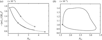
Figure 5(a) shows the dependence on
 $A_{yz}$
of the Reynolds stress at the central plane for
 $R_{S}=38.9$
and
 $A_{xz}=3$
, close to the initial bifurcation. Solutions exist only for
 $A_{yz}>1.1$
. The Reynolds stress decreases as
 $A_{yz}$
increases, and may approach a non-zero constant in the limit
 $A_{yz}\rightarrow \infty$
. The same is true for the velocity fluctuations (not shown). Note that, since the grid becomes relatively coarser as
 $A_{yz}$
increases, a finer
 $y$
grid is used for taller boxes (dashed lines), and that the good agreement of the results whenever the two grids overlap confirms numerical convergence.
The dependence on the streamwise aspect ratio
 $A_{xz}$
is shown in figure 5(b). Solutions exist for
 $1.58\lesssim A_{xz}\lesssim 3.29$
, which covers the range of box aspect ratios (
 $A_{xz}\approx 3$
) identified by Sekimoto et al. (Reference Sekimoto, Dong and Jiménez2016) to be good models for wall-bounded shear turbulence. It is interesting that the minimum aspect ratio for steady Nagata equilibrium solutions in plane Couette flow is
 $A_{xz}\approx 1.62$
at low Reynolds numbers (Jiménez et al.
Reference Jiménez, Kawahara, Simens, Nagata and Shiba2005), and that Deguchi (Reference Deguchi2015) showed that they exist only for
 $A_{xz}\gtrsim 1.5$
, even at high Reynolds numbers. On the other hand, Kawahara & Kida (Reference Kawahara and Kida2001) found unstable periodic orbits for somewhat shorter boxes,
 $A_{xz}=1.46$
.
Figure 6 shows the continuation along
 $R_{S}$
for
 $A_{xz}=3$
and several
 $A_{yz}$
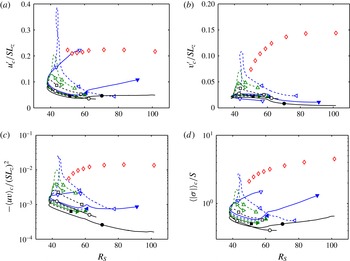
. The box-averaged statistics of LES (symmetric) turbulence are also shown for comparison. For
 $R_{S}\lesssim 60$
, those turbulence simulations occasionally become vertically localised around
 $y=0$
, but they spread again to fill the whole domain (see § 4.3). The box-averaged turbulence statistics in figure 6 include such locally quiescent regions, leading to weaker
 $v^{\prime }$
and
 $w^{\prime }$
fluctuations than would otherwise be obtained at the central plane. When
 $R_{S}\lesssim 50$
, LES turbulence often decays to laminar after these localisation events.
The velocity fluctuations for the upper-branch solutions are quite large in flat boxes and at low Reynolds number,
 $A_{yz}=1.5$
and
 $R_{S}\approx 45$
, but that behaviour disappears for taller boxes and saturates beyond
 $A_{yz}\approx 3$
. These large fluctuations are thus probably an effect of the shear-periodic boundary condition. This is also the range in which the shear periodicity results in the strongest temporal oscillations of the kinetic energy, of the order of 1 %, but we tested that the fluctuations in figure 6(a,c) are not due to the temporal variability. They are also present in the spacial average of instantaneous snapshots. The temporal oscillation of solutions with
 $A_{yz}>2$
is of the order of
 $10^{-5}$
.
The relatively poor scaling of the velocity fluctuations of the LES equilibria with
 $SL_{z}$
can be traced to the poor scaling of
 $|\unicode[STIX]{x1D70E}|/S$
. Figure 6(d) shows that the dimensionless strain rate of the upper-branch equilibria is roughly unity for
 $R_{S}=50$
–100, while that of turbulence is in the range of 2–5. It was shown by Sekimoto et al. (Reference Sekimoto, Dong and Jiménez2016) that, although
 $SL_{z}$
is the natural velocity scale for ‘good’ DNS boxes, the fluctuations in non-optimal boxes scale better with the friction velocity obtained from their total measured stress. In essence, the Reynolds stress and the velocity fluctuations scale with each other.
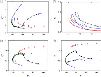
The same is true for LES and for equilibrium solutions. Figure 7(a,c,d) shows that the fluctuations collapse to a common curve in these ‘wall’ units. The vorticity components also scale well with
 $u_{\unicode[STIX]{x1D70F}}/l_{S}$
(not shown). In this normalisation, the velocity fluctuations of symmetric LES turbulence at
 $R_{S}=100$
are
 $u^{\prime +}\approx 2$
,
 $v^{\prime +}\approx 1.2$
and
 $w^{\prime +}\approx 1.4$
, which agree well with those at the top of the logarithmic layer of turbulent channels. When
 $R_{S}<60$
, the velocity fluctuations of the LES equilibria are not very different from those of turbulence, but we have seen that the lower-branch solutions tend to get concentrated around the critical layer as
 $R_{S}$
increases. Their statistics then become very different from turbulence.
Figure 7(b) is an enlargement of figure 7(a), showing the dependence on
 $A_{xz}$
of the minimum bifurcation Reynolds number of equilibria with
 $A_{yz}=3$
. It turns out that the bifurcation is more dependent on
 $A_{xz}$
than on
 $A_{yz}$
. At a fixed
 $A_{xz}=3$
, the minimum
 $R_{S}$
is
 $(38.11,38.00,37.94,37.91,37.89,37.90)$
for
 $A_{yz}=(1.33,1.5,1.64,1.8,2.0,3.0)$
, with a maximum scatter of 0.6 %. On the other hand, when
 $A_{yz}$
is fixed at 3,
 $R_{S}$
changes by 8 %, from 35.05 to 37.90, as
 $A_{xz}$
changes from 2 to 3.
(a,c,d) As in figure 6, but scaled by
 $u_{\unicode[STIX]{x1D70F}}$
at
 $y=0$
: (a,b)
 $u_{c}^{\prime +}$
, (c)
 $v_{c}^{\prime +}$
, (d)
 $w_{c}^{\prime +}$
. (b) Detail of (a): solid with
 $\triangle$
, red,
 $A_{xz}=2$
; solid with
 $\Box$
, blue,
 $A_{xz}=2.5$
; black with
 $\circ$
,
 $A_{xz}=3$
.

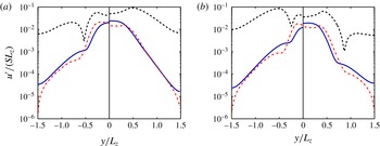
Velocity fluctuations for
 $A_{xz}=A_{yz}=3$
: (a)
 $R_{S}=50$
, (b)
 $R_{S}=62.5$
; only half of each plot is shown, using the symmetry in
 $y$
. Left side is lower branch. Right side is upper branch. Curves: - - - - (black),
 $u^{\prime }$
; —— (blue),
 $v^{\prime }$
; – - – - – (red),
 $w^{\prime }$
.

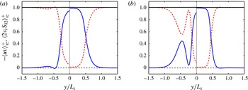
(a,b) As in figure 8, for the momentum balance: —— (blue),
 $\langle -uv\rangle _{xz}/u_{\unicode[STIX]{x1D70F}}^{2}$
; - - - - (red),
 $\langle 2\unicode[STIX]{x1D708}_{t}\overline{\unicode[STIX]{x1D70E}}_{xy}\rangle _{xz}/u_{\unicode[STIX]{x1D70F}}^{2}$
; —— (black), total stress.

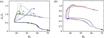
Height of the velocity streak, defined by the distance
 $d_{s}$
between the peaks of
 $u^{\prime }$
in the core part of the solutions in figure 8. Only peaks in the inner core are considered, and the secondary peaks in the outer one-component layer are ignored. (a) Plot for
 $A_{xz}=3$
and
 $A_{yz}=1.33,1.5,1.64,1.8,2,3$
. Lines and symbols as in figure 6. (b) Plot for
 $A_{xz}=2,2.5,3$
and
 $A_{yz}=3$
. Lines and symbols as in figure 7(b).

Vertically localised upper-branch solutions. Plots as in figure 3, for
 $A_{xz}=3,~A_{yz}=3$
and (a)
 $R_{S}=42.7$
and (b)
 $R_{S}=62.5$
.

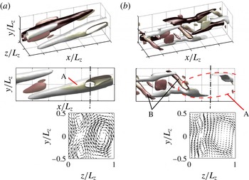
Isosurfaces of the second invariant of the velocity gradient (
 $Q=0.2Q_{max}$
) coloured by
 $\unicode[STIX]{x1D714}_{x}$
, with the same colour code as in the streamwise-averaged
 $\unicode[STIX]{x1D714}_{x}$
maps in the left panels of figure 11(a,b):
 $\unicode[STIX]{x1D714}_{x}<0$
(dark grey),
 $\unicode[STIX]{x1D714}_{x}>0$
(light grey). From top to bottom, each panel shows: a three-dimensional view, a side view of the region
 $0.5\leqslant z/L_{z}\leqslant 1$
, and a cross-section of cross-flow velocity vectors at
 $x/L_{z}=2.25$
, marked as a chain-dotted vertical line in the side views. The primary streamwise rollers visible in these cross-sections are not always compact enough to appear in the
 $Q$
isosurfaces and are marked as A in the lateral views. Flow as in figure 11(a,b). Only the active part,
 $|y|/L_{z}<0.5$
, is shown in all cases.

4.2 The structure of the upper-branch equilibria
We focus next on the flow structure of the vertically localised upper-branch equilibria in a box with
 $A_{xz}=3$
and
 $A_{yz}=3$
. The right-hand side of the two panels in figure 8 shows that the velocity fluctuations of these solutions decay exponentially away from
 $y=0$
, which is a common feature of localised solutions in other shear flows (Schneider, Gibson & Burke Reference Schneider, Gibson and Burke2010; Gibson & Brand Reference Gibson and Brand2014). The tail of
 $u^{\prime }$
is much stronger than those of
 $v^{\prime }$
and
 $w^{\prime }$
. This can be shown to be due to a streamwise-constant ‘streak’ of the streamwise velocity that can be approximated as a roughly sinusoidal spanwise perturbation of the mean profile,
 $u_{s}\sim \sin (2\unicode[STIX]{x03C0}z/L_{z})$
. This weak perturbation is the far tail of the stronger sinuous streak of
 $u$
concentrated near
 $y=0$
and, because it is almost independent of
 $x$
, is essentially independent of
 $v$
,
 $w$
and the shear. The left-hand part of both panels in figure 8 represents lower-branch solutions, which share many of the characteristics of the upper branch. As the Reynolds number increases, all structures become more complex, as seen in figure 8(b) and later in figures 11 and 12, and the core of the structures develop substructures that could perhaps be interpreted as a first indication of a turbulent cascade. The momentum balance of these flows is shown in figure 9. The Reynolds stress is dominant in the core,
 $|y|/L_{z}<0.5$
, but only the mean shear
 $\text{d}U/\text{d}y$
contributes to the eddy viscosity in the outer part.
Figure 10 presents the height of the velocity streak for the different equilibria, defined as twice the distance to
 $y=0$
of the first maximum of the
 $u^{\prime }$
profile of the solutions in figure 8. The height of the lower-branch streak stays roughly constant below
 $R_{S}\approx 50$
, and approaches zero quickly above that limit, as the solutions collapse to the critical layer. In contrast, the height of upper-branch solutions increases drastically near the bifurcation point and reaches a maximum near
 $R_{S}\approx 45$
. This is also the range in which the velocity fluctuations become very strong in figure 6, and only appears in flat boxes with
 $A_{yz}=1.33{-}1.64$
. We argued in the discussion of figure 6 that upper-branch solutions tend to be limited by the height of these flat boxes, and figure 10(a) confirms this interpretation by showing that the maximum height of the streak reaches the box height. On the other hand, this interaction does not take place when
 $A_{yz}\gtrsim 2$
, confirming the independence of those solutions from the box dimensions.
The flow structures of the upper-branch solutions at
 $R_{S}=42.7$
and 62.5 are visualised in figures 11 and 12. The streak is represented by the
 $\overline{u}=0$
isosurface that spans
 $|y|/L_{z}<0.5$
in figure 11 (see also figure 3
a,b). The corresponding vortical structures are located in the flanks of the streak, as seen in the streamwise-averaged cross-stream maps of
 $\unicode[STIX]{x1D714}_{x}$
in figure 11. The vortical structures are shown by themselves in figure 12, and are surprisingly complex for an equilibrium solution. This is especially true for the higher-Reynolds-number case in figures 11(b) and 12(b), which appear to include a double structure that is nevertheless in equilibrium. In fact, there is a first indication of two separate scales in these flow fields. The smaller tube-like vortical structures are isosurfaces of the second invariant of the velocity gradient tensor (
 $Q$
criterion), and are coloured by the streamwise vorticity. They do not always coincide with the larger-scale structures of the cross-stream velocity, which are visible in the cross-sections in the bottom part of figure 12. These ‘rollers’ are too diffuse to appear in the
 $Q$
-map, which may actually appear empty in the region in which the roller is dominant (see the region labelled as A in the side view in figure 12
b, and note that, because of the symmetry of the flow, a mirror-symmetric arrangement is present in the upstream half of the box). On the other hand, it is clear from the cross-sections that the roller dominates the velocity field.
The low-Reynolds-number solution in figure 12(a) shows that the
 $Q$
-vortices are parts of the larger streamwise rollers that have been sheared and stretched by the mean flow. The cross-sections in the bottom part of figure 12 show that these vortices are long enough to spill into neighbouring periodic boxes, so that they appear as double in the cross-section. The inclination angle of these streamwise rollers and vortices is roughly 15
 $^{\circ }$
at all Reynolds numbers. In the higher-Reynolds-number case in figure 12(b), the streamwise vortices are strong enough to create new vortices, roughly perpendicular to them, which are labelled as B in the side view in figure 12(b). They rotate in the opposite sense to the primary streamwise rollers and are aligned in the direction of the strain produced by them. A similar generation mechanism of secondary smaller vortices has been investigated in the homogeneous isotropic turbulence (Goto Reference Goto2012).
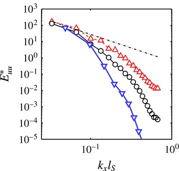
The velocity spectra in figure 13 show that the upper-branch solutions acquires more small-scale structures as
 $R_{S}$
increases, approaching the spectrum of turbulence LES at similar Reynolds numbers. Even though the turbulence state has more small scale, the large-scale end of its spectrum is quantitatively similar to the upper-branch solutions.
Streamwise velocity spectrum
 $E_{uu}^{\ast }=E_{uu}(k_{x})\unicode[STIX]{x1D700}^{-2/3}l_{S}^{-5/3}$
as a function of
 $k_{x}l_{S}$
:
 $\triangledown$
(blue), upper-branch solution at
 $R_{S}=42.7$
;
 $\circ$
(black), upper-branch solution at
 $R_{S}=62.5$
;
 $\triangle$
(red), turbulence LES at
 $R_{S}=62.5$
. The dash-dotted line represents the inertial theory
 $E_{uu}^{\ast }(k_{x})=0.6(l_{S}k_{x})^{-5/3}$
. The spectra and dissipation rates of the upper-branch solutions are averaged over
 $|y|/L_{z}<0.5$
.

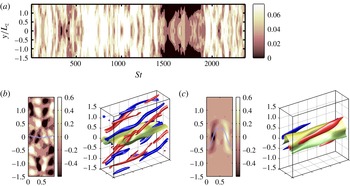
(a) Vertical velocity fluctuation intensity profiles,
 $\langle v^{2}\rangle _{xz}^{1/2}/(SL_{z})$
, as a function of
 $y/L_{z}$
and
 $St$
. The contours are
 $[0.02:0.02:0.08]$
, and the mean value of
 $v^{\prime }$
is approximately
 $0.07SL_{z}$
(see figure 6). Here
 $A_{xz}=3$
,
 $A_{yz}=3$
and
 $R_{S}=50$
. (b) Homogeneous turbulence at
 $St=1318$
. (c) Localised state at
 $St=1525$
. The left panels in (b) and (c) show the streamwise-averaged
 $\unicode[STIX]{x1D714}_{x}$
, and the right ones show isosurfaces of
 $\unicode[STIX]{x1D714}_{x}$
and
 $\overline{u}$
, as in figure 3.

4.3 Intermittent visiting of turbulence to vertically localised states
We mentioned in § 4.1 that, when
 $R_{S}$
is relatively low, LES turbulence collapses intermittently to a localised state around
 $y=0$
, and that these states persist for a long time when
 $R_{S}\gtrsim 50$
. These are the statistics plotted as diamonds in figure 6. Figure 14(a) shows the temporal evolution of the profile of local
 $v^{\prime }$
. Light colours represent active turbulent regions and dark ones are overdamped ‘laminar’ areas. Localised turbulence occurs when laminarisation does not extend over the whole height of the box, such as in
 $St=1500{-}2000$
.
Note that localisation only takes place in flows with sinuous symmetry, so that the profiles are symmetric with respect to
 $y=0$
, but that the symmetry allows localisation either at the centre plane,
 $y=0$
, or at the top or bottom of the box,
 $y=\pm L_{y}/2$
. The strongest event in figure 14(a) is localised at
 $y=0$
 $(St=1500{-}2000)$
, but there are several minor ones (e.g. at
 $St\approx 400$
) localised at the top of the box.
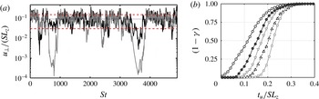
The structure of the flow at a fully turbulent moment is shown in figure 14(b), and shows that vorticity is spread over the whole box. Figure 14(c) represents the flow during a localisation event. Its similarity to the localised lower-branch equilibrium solutions is striking. Since we saw in § 3 that these solutions are edge states whose unstable manifold leads to bursting, it is tempting to interpret localisation as the occasional approach of fully developed turbulence to the localised solution along its stable manifold, and its later spreading to a fully turbulent state along the unstable manifold. A similar behaviour was reported in a plane channel by Itano & Toh (Reference Itano and Toh2001), and Kawahara (Reference Kawahara2005) used the occasional approaches to the edge state to laminarise turbulent Couette flow.
(a) The local cross-flow velocity fluctuation intensity
 $u_{\bot }$
defined in (4.1) at: (black)
 $y=L_{y}/2$
(
 $u_{t}$
); (grey)
 $y/L_{z}=0$
(
 $u_{c}$
). The black dashed line is the mean value,
 $\langle u_{\bot }\rangle$
, and the red dashed lines are
 $\langle u_{\bot }\rangle \pm \unicode[STIX]{x1D70E}$
, where
 $\unicode[STIX]{x1D70E}$
is the standard deviation. They are defined as averages over the centre and top of the box, as explained in the text. (b) The intermittency factor
 $(1-\unicode[STIX]{x1D6FE})$
, where
 $\unicode[STIX]{x1D6FE}$
is defined in (4.2): —
 $\circ$
—,
 $R_{S}=50.0$
; —
 $\bullet$
—,
 $R_{S}=52.6$
; —
 $\triangledown$
— (grey),
 $R_{S}=55.5$
; – –
 ${\vartriangle}$
– –,
 $R_{S}=62.5$
; —
 $\Box$
— (grey),
 $R_{S}=101.6$
.

We next quantify the frequency of these localisation events. Figure 15(a) shows the evolution of the transverse velocity fluctuation intensity, defined as
 $$\begin{eqnarray}u_{\bot }(y)\equiv (\langle v^{2}\rangle _{xz}+\langle w^{2}\rangle _{xz})^{1/2}.\end{eqnarray}$$
The darker line is the intensity at
 $y=0$
, and the lighter one is the intensity at
 $y=\pm L_{y}/2$
. The thin straight solid and the dashed lines are the mean,
 $\langle u_{\bot }\rangle$
, and deviation,
 $\unicode[STIX]{x1D70E}$
, which are the averages of these two positions. By defining
 $u_{c}=u_{\bot }(0)$
and
 $u_{t}=u_{\bot }(L_{y}/2)$
, fully turbulent profiles should have large
 $u_{c}\approx u_{t}\approx \langle u_{\bot }\rangle$
, while localised states are characterised by having one of these intensities much weaker than the fully turbulent one. The quantity
 $$\begin{eqnarray}\unicode[STIX]{x1D6FE}\equiv \int _{t_{u}}^{\infty }\int _{t_{u}}^{\infty }P(u_{c},u_{t})\,\text{d}u_{c}\,\text{d}u_{t},\end{eqnarray}$$
where
 $P(u_{c},u_{t})$
is the joint probability density function of both intensities, and
 $t_{u}$
is a threshold, measures the probability that the points
 $y=0$
or
 $L_{y}/2$
are turbulence according to
 $u_{c}\geqslant t_{u}$
or
 $u_{t}\geqslant t_{u}$
. Since the localised state has the overdamped laminar region, which appears intermittently as shown in figure 15(a),
 $(1-\unicode[STIX]{x1D6FE})$
indicates the intermittency factor of the localised turbulence. Figure 15(b) shows that the frequency of localisation decreases as
 $R_{S}$
increases.
5 Conclusions
We have performed LES of SS-HST in a subspace with sinuous symmetry, and found equilibrium solutions with the same symmetry. We use a Smagorinsky-type model with no molecular viscosity, which is not required because of the absence of walls, so that the eddy viscosity
 $\unicode[STIX]{x1D708}_{t}\equiv l_{S}^{2}|S|$
acts as the only energy sink. It is parametrised by a mixing length
 $l_{S}$
that plays the role of the Kolmogorov scale in LES, independent of the numerical grid. For the grids used in this study, the flow is independent of the numerical resolution. The integral scale in the LES of the SS-HST is comparable to the spanwise box dimension,
 $L_{0}\approx 0.4L_{z}$
, as in the DNS of the same flow in Sekimoto et al. (Reference Sekimoto, Dong and Jiménez2016) and as in wall-bounded turbulence in spanwise-limited boxes (Flores & Jiménez Reference Flores and Jiménez2010). The effective Kolmogorov scale is
 $\unicode[STIX]{x1D702}_{t}\approx 0.9l_{S}$
, and the velocity fluctuations scale well with
 $SL_{z}$
, as in DNS. Even if we introduce the molecular viscosity in our LES, considering the effective Kolmogorov length,
 $\widetilde{\unicode[STIX]{x1D702}_{t}}\approx \widetilde{l_{S}}\equiv l_{S}(1+\unicode[STIX]{x1D708}/\unicode[STIX]{x1D708}_{t})^{1/2}$
(see Pope Reference Pope2000), the results would not change as long as
 $\unicode[STIX]{x1D708}$
is small enough with respect to the mean
 $\unicode[STIX]{x1D708}_{t}$
.
The length-scale ratio
 $R_{S}=L_{z}/l_{S}$
is used as a continuation parameter for LES equilibria, playing the role of a Reynolds number, and it is found that vertically localised equilibrium solutions appear by a saddle-node bifurcation at
 $R_{S}=37.9$
for
 $A_{xz}=3$
. The dependence of the equilibrium solutions on the box aspect ratios has been investigated, and it is revealed that both lower- and upper-branch solutions tend to localise vertically around the central plane of the box. The initial bifurcation point is roughly independent of
 $A_{yz}$
, and much more dependent on
 $A_{xz}$
. These solutions exist in
 $1.58\lesssim A_{xz}\lesssim 3.29$
and
 $A_{yz}>1.1$
at
 $R_{S}=39.0$
. This range of aspect ratios spans those found by Sekimoto et al. (Reference Sekimoto, Dong and Jiménez2016) to be good models for unconstrained shear flows in general. The minimum limit of
 $A_{xz}\gtrsim 1.6$
is also similar to those found for the existence of equilibria in plane Couette flow by Nagata (Reference Nagata1990) and Deguchi (Reference Deguchi2015). These and other authors have mentioned that such equilibria can be embedded in general unbounded shear flows, but the localisation of the present solution in an approximately linear shear is almost surely due to the interaction with the local eddy-viscosity profile. As
 $R_{S}$
increases, the lower-branch solutions take the form of a critical layer, such as those found in previous works on wall-bounded flows (Wang et al.
Reference Wang, Gibson and Waleffe2007; Viswanath Reference Viswanath2009; Deguchi & Hall Reference Deguchi and Hall2014b
), and described by VWI theory (Hall & Smith Reference Hall and Smith1991; Hall & Sherwin Reference Hall and Sherwin2010).
The length scales of the LES equilibria are
 $l_{S}$
for the small scale and
 $L_{z}$
for the large one, as in LES turbulence. The comparison of the contribution of the eddy viscosity and of the Reynolds stress to the momentum balance reveals that the former is weak within the localised equilibrium solutions, and predominates outside it. The velocity fluctuations of the present equilibria are substantially smaller than those of self-sustaining turbulence, especially in the VWI limit, and do not scale well with
 $SL_{z}$
. However, they scale well with their own
 $u_{\unicode[STIX]{x1D70F}}$
, with similar values to those of wall-bounded flows expressed in wall units.
At low Reynolds numbers, lower-branch solutions act as edge states. Although their eigenvalue structure is more complicated than a simple saddle, one of the unstable directions of the saddle leads to an exponential burst and to chaotic turbulence, while the other laminarises. In turbulent LES, the flow occasionally collapses to a localised state that resembles the equilibrium solutions. Depending on the Reynolds number, the outcome of these events is more often reinjection to turbulence, or laminarisation.
Upper-branch solutions have tall velocity streaks associated with small-scale vortices, whose complication increases with increasing
 $R_{S}$
. It is interesting that, even at the relatively low
 $R_{S}\approx 62$
, small secondary vortices begin to appear in these solutions, aligned perpendicularly to the primary streamwise rollers in a manner strongly reminiscent of the multiscale process frequently invoked as models for the turbulent cascade. Further continuations to higher
 $R_{S}$
are hardly successful, probably because of their increasing complexity and instability, which is a similar limitation to the one we encounter when searching for dynamically important invariant solutions in the Navier–Stokes computations at high Reynolds numbers.
In all, the localised LES equilibria discovered here represent a promising model for generic isolated turbulent structures in shear flows. Most intriguingly, the higher Reynolds numbers contain what appear to be the first stages of a multiscale cascade.
Acknowledgements
This research has been funded by the European Research Council grants ERC-2010.AdG-20100224 and ERC-2014.AdG-669505. We are grateful to G. Kawahara for early discussions.
Appendix. Linear stability analysis of equilibria in LES
We discuss in this section the linear stability of the vertically localised symmetric equilibria described in the body of the paper. Even if we saw in figure 7(a) that the continuation diagram of these solutions is roughly independent of the vertical box aspect ratio, it turns out that this aspect ratio affects the stability of the equilibria, especially that of the upper-branch solutions. Since we showed in figure 10 that these solutions are tall enough to span the full height of the box, especially in the case of the flatter boxes with
 $A_{yz}\leqslant 1.5$
, the artificial interactions with the shear-periodic copies in
 $y$
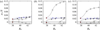
is inevitable. Figure 16 shows the distribution of a few of the least stable eigenvalues obtained from the linear stability analysis of equilibria with
 $A_{xz}=3$
and
 $A_{yz}=1.5,~2$
and 3. The vertically localised equilibrium solution appears through a saddle-node bifurcation as
 $R_{S}$
increases. The upper branch always has at least one pair of unstable complex-conjugate modes, and becomes more stable as
 $A_{yz}$
decreases.
In taller boxes, with
 $A_{yz}=2{-}3$
, the distribution of unstable eigenvalues of the upper-branch solutions is not strongly affected by the box aspect ratio, in rough agreement with the criterion,
 $A_{xz}\lesssim 2A_{yz}$
, found in previous DNS studies of SS-HST to be required for box independence (Sekimoto et al.
Reference Sekimoto, Dong and Jiménez2016).
The real-part of non-dimensional eigenvalues obtained by the linear stability analysis of equilibria for
 $A_{xz}=3$
and (a)
 $A_{yz}=1.5$
, (b)
 $A_{yz}=2$
, (c)
 $A_{yz}=3$
:
 $\triangledown$
, lower branch;
 $\circ$
, upper branch. The filled (open) symbols represent real (complex-conjugate) modes. Positive values represent unstable modes, and the square is the bifurcation point.