

1. Introduction
Granular aggregates of various geometric configurations like size, shape or surface roughness are prone to segregation when sheared, shaken or vibrated, which is called particle segregation. This can be found in nature, industries and even our daily life, e.g. wet snow avalanche (Bartelt & McArdell Reference Bartelt and McArdell2009), debris flow (Iverson Reference Iverson1997), pharmaceutical and chemical processes (Khakhar, McCarthy & Ottino Reference Khakhar, McCarthy and Ottino1997; Ottino & Khakhar Reference Ottino and Khakhar2000; Schlick et al. Reference Schlick, Fan, Umbanhowar, Ottino and Lueptow2015b), and the so-called ‘Brazil nut effect’ in our kitchens (Rosato et al. Reference Rosato, Strandburg, Prinz and Swendsen1987; Gajjar et al. Reference Gajjar, Johnson, Carr, Chrispeels, Gray and Withers2021). In some cases, this effect is desirable by segregation or classification (Jiang et al. Reference Jiang, Wu, Hu, Fu, Chen and Wang2021). However, in many other processes aiming for a homogeneous blend, the resulting non-uniformity is usually undesirable and should be eliminated . To this end, it is of practical significance to have better understanding of the de-mixing process (Trewhela, Gray & Ancey Reference Trewhela, Gray and Ancey2021b; Xu et al. Reference Xu, Yoshinaga, Tsunazawa and Tokoro2021).
Many factors are deemed responsible for particle segregation, including convection (Ehrichs et al. Reference Ehrichs, Jaeger, Karczmar, Knight, Kuperman and Nagel1995), fluidization (Schröter et al. Reference Schröter, Ulrich, Kreft, Swift and Swinney2006), clustering (Mullin Reference Mullin2000), and gravity-driven segregation. Among these, the last is recognized as the most dominant mechanism (Yang et al. Reference Yang, Zheng, Bai and Yu2021). The gravity-driven segregation is subject to the variance in the density or grain size. The former is intuitive and easily understandable, i.e. the particles with smaller density float to the top, while the heavier particles sink to the bottom due to the buoyancy effect. In contrast, the size-driven segregation is less straightforward and involves two processes. The first phase is termed kinetic sieving (Drahun & Bridgwater Reference Drahun and Bridgwater1983). At this stage, the large particles will relocate under shearing and give rise to some gaps, through which the small grains can penetrate downwards easily. Subsequently, all particles are leveraged to its adjacent layer due to the imbalance in contact forces on an individual grain. This process is named squeeze expulsion and believed to be size-insensitive (Savage & Lun Reference Savage and Lun1988). As time marches, the fine particles cluster at the bottom of the granular body, while the large ones tend to appear at the top, leading to the final inhomogeneous particle configuration. Due to its dominant role in particle segregation, the size-driven mechanism has attracted much attention. A comprehensive review on particle segregation in dense granular flows was provided recently by Gray (Reference Gray2018), which is highly recommended for readers interested in this topic.
Gray & Thornton (Reference Gray and Thornton2005) proposed a continuum-transport-based theoretical framework for the segregation-driven shallow granular free-surface flow. This approach starts from the mass and momentum conservation equations for each constituent, and introduces the percolation velocity using the interaction drag between phases. Later, Gray & Chugunov (Reference Gray and Chugunov2006) extended this theory to include the diffusion effect. This model is applied widely, and is capable of predicting qualitatively or quantitatively the results from experiments or simulations in various configurations, such as plug (Thornton, Gray & Hogg Reference Thornton, Gray and Hogg2006), annular shear (May et al. Reference May, Golick, Phillips, Shearer and Daniels2010) and chute (Wiederseiner et al. Reference Wiederseiner, Andreini, Épely-Chauvin, Moser, Monnereau, Gray and Ancey2011). However, as an analytical method, it needs some presumptions of the flow kinematics for simplification, limiting its applicability to the specific flow configurations. Another approach on this topic goes to the particle scale simulation using discrete models such as the discrete element method (DEM) (Brandao et al. Reference Brandao, Lima, Santos, Duarte and Barrozo2020). The DEM captures each particle trajectory in simulation, thus providing microscopic insight into the problem. For example, Thornton et al. (Reference Thornton, Weinhart, Luding and Bokhove2012) studied the relation between the segregation Péclet number (ratio of the segregation velocity to diffusion) and the particle-size ratio in a bidisperse mixture. Fry et al. (Reference Fry, Umbanhowar, Ottino and Lueptow2018) investigated the effect of the confining pressure on segregation of granular material. The DEM is also used to determine some macroscopic quantities for the continuum models (Fan et al. Reference Fan, Schlick, Umbanhowar, Ottino and Lueptow2014; Tunuguntla, Weinhart & Thornton Reference Tunuguntla, Weinhart and Thornton2017). Despite the insight of such DEM simulations for the size-driven particle migration, however, the notorious high computation cost limits the applicability of the DEM to small-scale granular flow modelling. Thus it is of urgency to develop a generic method based on fundamental flow dynamics without the limitation of the system configuration and problem scale.
Continuum-model-based numerical methods are often used in computational fluid dynamics and computational solid mechanics for large-scale problems ascribed to their outstanding calculation efficiency. In the field of polydisperse granular simulation, two theoretical frameworks can be found. One is based on the mixture theory, which takes multisized granular media as spatially overlapped continua specified with different particle sizes, and introduces the source term such as the drag force in the momentum conservation equations to mimic the interplay between different constituents. Within this framework, Huang, Kao & Kuo (Reference Huang, Kao and Kuo2013) studied the solid–solid–gas three-phase particle segregation in a rotating drum using the Eulerian continuum approach. The other framework, adopted in this study, regards the particle aggregates as a single-phase system with varying concentration of constituents, and brings in the convective–diffusive transport equation governing the evolution of the concentration. More works have been conducted with the latter method, as the transport equation has been well studied in the multidisperse granular flow problem (Liu, Gonzalez & Wassgren Reference Liu, Gonzalez and Wassgren2018; Yang et al. Reference Yang, Zheng, Bai and Yu2021). For instance, Barker et al. (Reference Barker, Rauter, Maguire, Johnson and Gray2021) implemented two-way coupling of segregation–diffusion–advection equations with partially regularized incompressible  $\mu (I)$ rheology, and investigated numerically the inclined slope flow and square rotating drum in OpenFOAM. However, it is found that most of these studies adopt hybrid grid-based numerical methods, such as the combination of the Eulerian finite-element method (FEM) and the finite difference method, with the former updating the velocity information, whereas the latter solves the transport equation. Consequently, several drawbacks are inherent in such procedures due to the nature of the Eulerian grids, including (1) the difficulty in obtaining the temporal evolution of the field variables on a fixed particle, (2) the high computational cost and inaccuracy in tracking the free surface of the granular flow, and (3) cumbersomeness to treat irregular or complex geometries. Also, the mixed numerical methods have often complex formulations and are difficult to implement. To overcome these disadvantages, we present a mesh-free solver based on the smoothed particle hydrodynamics (SPH) in the current study.
The SPH method is a Lagrangian particle-based mesh-free method that is suitable for problems involving large deformation and free-surface flows like the granular flow to be discussed in this study, because (1) it can avoid the instability caused by the large deformation or grid distortion in the conventional grid-based methods, and (2) no effort is needed to track the free surface thanks to the inherent property as a Lagrangian method. Initially, SPH was invented to solve problems in astrophysics in the 1970s (Gingold & Monaghan Reference Gingold and Monaghan1977; Lucy Reference Lucy1977). After almost half a century of development, it has been used in various walks of science and engineering, including cardiovascular medicine (Zhang et al. Reference Zhang, Wang, Rezavand, Wu and Hu2021), porous media flow (Peng et al. Reference Peng, Xu, Wu, Yu and Wang2017), high-explosive explosion (Liu et al. Reference Liu, Liu, Zong and Lam2003), the food industry (Harrison et al. Reference Harrison, Eyres, Cleary, Sinnott, Delahunty and Lundin2014), and geohazard prediction (Fourtakas & Rogers Reference Fourtakas and Rogers2016). In the past decades, SPH is also widely used in simulating the granular avalanche and debris flow. Despite the success of this method in multiple disciplines, the explicit time integration scheme adopted in SPH leads to low computation efficiency, in particular when it comes to large-scale three-dimensional problems. Fortunately, the locality property of this method makes it quite suitable for parallel computation. In this study, the GPU acceleration solution empowered by an NVIDIA generic graphic card will be adopted due to its better accessibility, availability and affordability compared with CPU clusters that are usually used in supercomputers.
In the remainder of this paper, the mathematical framework of the size-driven particle segregation will be developed, followed by the introduction of the constitutive model for the granular aggregates, in § 2. Then a brief introduction to the SPH formulation will be given in § 3. Section 4 describes the proposed hybrid continuum surface reaction scheme, which is necessary for realizing the inhomogeneous Neumann boundary condition for each granular constituent. In § 5, the developed solver is examined with the shear box experiment conducted by Van der Vaart et al. (Reference Van der Vaart, Gajjar, Épely-Chauvin, Andreini, Gray and Ancey2015). In § 6, the proposed SPH model is applied to investigate the segregation dynamics in a rotating drum filled with a bidisperse-sized granular assembly. Finally, some conclusions are summarized in § 7 to close the study.
2. Mathematical framework
The bidisperse granular assembly consists of three domains, i.e. the space occupied by the large grains (L), the small ones (S), and the interstitial fluid (F), as shown in figure 1. The volume fractions for each constituent are  $\phi ^{L}$,
 $\phi ^{S}$ and
 $\phi ^{F}$, with the superscript denoting the corresponding phase. In this study, the interstitial fluid is air, and its effect on the particle-size segregation is ignored. Since the concern lies in the evolution of the local grain distribution, the following volumetric concentration is introduced as an indicator to reflect the particle-size segregation:
 \begin{equation} C^{X}=\frac{\phi^X}{\phi^{L}+\phi^{S}}, \end{equation}
where  $X={\rm L}, {\rm S}$, representing the specific grain size. The volume concentration is
 $C^{X}\in [0,1]$, and the two extremes
 $C^{X}=0$ or 1 denote the full segregation. Based on the above concentration definition, the following constraint holds everywhere of the calculation domain:
 \begin{equation} C^{L}+C^{S}=1. \end{equation}
Schematic diagram of a bidisperse granular assembly, in which L, S and F refer to large grains, small grains, and interstitial fluid, respectively.

2.1. Granular flow model
Within the framework of continuum mechanics, the governing equations dictating a granular flow include the mass conservation
 \begin{equation} \frac{{\rm d}\rho}{{\rm d} t}=-\rho\,\boldsymbol{\nabla}\boldsymbol{\cdot}\boldsymbol u, \end{equation}
and the linear momentum conservation
 \begin{equation} \frac{{\rm d}\boldsymbol u}{{\rm d} t}=\frac{1}{\rho}\,\boldsymbol{\nabla}\boldsymbol{\cdot}\boldsymbol\sigma+\boldsymbol g. \end{equation}
Here,  ${\rm d}(\ \cdot\ )/{\rm d} t=\partial (\ \cdot\ )/\partial t+\boldsymbol u\boldsymbol {\cdot }\boldsymbol {\nabla }(\ \cdot\ )$ is the material derivative,
 $\rho$ represents the bulk density;
 $\boldsymbol u$ is the velocity vector;
 $\boldsymbol \sigma$ denotes the stress tensor; and
 $\boldsymbol g$ refers to gravity, which is the most common external body force in granular flows. In this work, the granular mass is assumed incompressible, i.e. the bulk density
 $\rho$ remains constant, so (2.3) can be deactivated.
Often, granular flow is considered within hydrodynamics by Navier–Stokes equations, in which the non-Newtonian viscosity is deployed to describe the behaviour of granular material (Gilberg & Steiner Reference Gilberg and Steiner2020). However, such a model is incompatible with the solid-like behaviours of the granular mass in the quasi-static state (Yang et al. Reference Yang, Zheng, Bai and Yu2021). Therefore, we use a regularized  $\mu (I)$-rheology-based elastoplastic model in this study (Zhu, Peng & Wu Reference Zhu, Peng and Wu2022a). Details will be presented in § 2.3.
2.2. Segregation–diffusion model
To close the governing equations for the segregation dynamics of a bidisperse system, we need the so-called segregation–diffusion equation proposed by Gray & Chugunov (Reference Gray and Chugunov2006), which is formulated initially in the Eulerian framework. In this work, we first propose the following Lagrangian description:
 \begin{equation} \frac{{\rm d}C^{S}}{{\rm d}t}=-C^{S}\,\boldsymbol{\nabla}\boldsymbol{\cdot}\boldsymbol u-\boldsymbol{\nabla}_{g}Q+\boldsymbol{\nabla}\boldsymbol{\cdot}(D\,\boldsymbol{\nabla} C^{S} ). \end{equation}
In this equation,  $\boldsymbol {\nabla }_{g}$ denotes the gradient along the direction of gravity;
 \begin{equation} Q=VF \end{equation}
denotes the segregation flux, with  $V$ the segregation velocity, and
 $F$ the segregation function, whose specific expression will be given subsequently; and
 $D\,\boldsymbol {\nabla } C^{S}$ is the diffusion flux, with
 $D$ the diffusivity. The segregation velocity
 $V$ and diffusivity
 $D$ have similar scaling relations with the shear rate magnitude
 $\dot \gamma$ and average grain diameter
 $d_{avg}$ such that (Savage & Dai Reference Savage and Dai1993; Hajra & Khakhar Reference Hajra and Khakhar2002)
 \begin{equation} D=\chi_{D}\dot\gamma d_{avg}^2,\quad V=\chi_{V}\dot\gamma d_{avg}. \end{equation}
Here,  $\chi _{D}$ and
 $\chi _{V}$ are material coefficients;
 $\dot \gamma =\sqrt {2\dot {\boldsymbol e}:\dot {\boldsymbol e}}$ (with
 $:$ denoting the tensor inner product), where
 $\dot {\boldsymbol e}=\dot {\boldsymbol \varepsilon }-\dot \varepsilon _v\boldsymbol{\mathsf{I}}$ represents the deviatoric strain rate, with
 $\dot {\boldsymbol \varepsilon }=0.5(\boldsymbol u\,\boldsymbol {\nabla }+\boldsymbol {\nabla }\boldsymbol u)$ and
 $\dot \varepsilon _v=\textrm {tr}(\dot {\boldsymbol \varepsilon })/3$ (with
 $\textrm {tr}(\ \cdot\ )$ denoting the trace), and
 $\boldsymbol{\mathsf{I}}$ is the identity tensor:
 $d_{avg}=d^{S}C^{S}+d^{L}C^{L}$ with
 $d$ referring to the grain diameter. It should be noted that (2.7a,b) are indeed simplified, as both segregation velocity and diffusivity are found to rely on many other factors, such as frictional coefficient, inertial number, lithostatic pressure and grain radius ratio (Fry et al. Reference Fry, Umbanhowar, Ottino and Lueptow2019; Bancroft & Johnson Reference Bancroft and Johnson2021; Trewhela, Ancey & Gray Reference Trewhela, Ancey and Gray2021a). Also, in some studies,
 $V$ and
 $D$ are taken as constants, resulting in consistent agreement with experimental data (Van der Vaart et al. Reference Van der Vaart, Gajjar, Épely-Chauvin, Andreini, Gray and Ancey2015; Yang et al. Reference Yang, Zheng, Bai and Yu2021). Therefore, the effect of using constant or functional forms of
 $V$ and
 $D$ will be discussed in § 5. From (2.5), we can identify three factors that influence the temporal evolution of the local concentration of the small-size grain on a material point. The first term on the right-hand side of (2.5) reflects the contribution from the volume change, while the second accounts for the particle-size segregation, and the last for diffusive remixing. As mentioned above, this study is restricted to the incompressible granular flow, so that the first term on the right-hand side in (2.5) can be disregarded. Since the unity condition, i.e. (2.2), holds everywhere, and only
 $C^{S}$ is utilized in the rest of the paper, the superscript is omitted for brevity.
We proceed to consider the segregation function in (2.5). The following quadratic segregation function is used in a number of studies (Dolgunin & Ukolov Reference Dolgunin and Ukolov1995; Gray & Thornton Reference Gray and Thornton2005; Fan et al. Reference Fan, Schlick, Umbanhowar, Ottino and Lueptow2014):
 \begin{equation} F=C(1-C). \end{equation}
Equation (2.8) is also named the symmetric flux function as it is symmetric about  $C=0.5$, where both large and small grains have equal but opposite segregation flux. Despite its success in modelling segregation, the quadratic form may sometimes deviate from reality. For instance, Golick & Daniels (Reference Golick and Daniels2009) observed that the downward penetration of a small grain through a bidisperse matrix in an annular ring shear cell is faster than the rising of a large grain through the same matrix. Likewise, the percolation rate is observed noticeably lower for a large intruder migrating through a dissimilar granular matrix in a shear box than for a small intruder (Trewhela et al. Reference Trewhela, Ancey and Gray2021a). Based on the experimental observation, Gajjar & Gray (Reference Gajjar and Gray2014) proposed the asymmetric flux model
 \begin{equation} F=AC(1-C)(1-\kappa C), \end{equation}
where the parameter  $\kappa \in [0,1)$ controls the degree of asymmetry. The constant
 $A$ is chosen to ensure that the maximum flux is the same as for the symmetric flux function. Two sets of parameters
 $A$ and
 $\kappa$ (i.e.
 $A=1.0$,
 $\kappa =0$ and
 $A=1.6$,
 $\kappa =0.89$) are utilized in this study, and the corresponding segregation functions are demonstrated schematically in figure 2. Notice that (2.9) reduces to (2.8) in the case
 $A=1$ and
 $\kappa =0$. Also, in the case of asymmetric segregation flux, the cubic relation between
 $F$ and
 $C$ can lead to remarkable errors if (2.9) is substituted directly into (2.5) within the SPH framework. This is due to the complexity of high order between the segregation flux
 $Q$ and coordinates. A detailed explanation is presented in Appendix A. For a better approximation, we modify the segregation–diffusion equation as
 \begin{equation} \dfrac{{\rm d}C}{{\rm d}t}=-V\mathcal{F}\,\boldsymbol{\nabla}_{g}C-F\,\boldsymbol{\nabla}_{g}V+\boldsymbol{\nabla}\boldsymbol{\cdot}(D\,\boldsymbol{\nabla} C ), \end{equation}
in which  $\mathcal {F}={\partial F}/{\partial C}=A( 3\kappa C^2-2( 1+\kappa )C+1 )$.
Quadratic and cubic segregation functions.

2.3. Regularized  $\mu (I)$-rheology-based elastoplastic model

In this subsection, the regularized  $\mu (I)$-rheology-based elastoplastic model with Drucker–Prager yield surface, first put forward in Zhu et al. (Reference Zhu, Peng and Wu2022a), is introduced briefly for the sake of self-containment. This model is featured with the pressure-dependent yield function written as
 \begin{equation} f(\,p,J_2)=\sqrt{J_2}-k_\mu p, \end{equation}
where  $p={\rm tr}(\boldsymbol \sigma )/3$ is the hydrostatic pressure;
 $J_2 = 0.5\boldsymbol s:\boldsymbol s$ represents the second invariant of the deviatoric stress
 $\boldsymbol s=\boldsymbol \sigma -p\boldsymbol{\mathsf{I}}$; and
 $k_\mu$ is the constitutive parameter related to the Mohr–Coulomb model through
 \begin{equation} k_\mu=\frac{3\mu}{\sqrt{9+12\mu^2}}, \end{equation}
in which  $\mu$ is the frictional coefficient. In the standard Drucker–Prager model,
 $\mu$ is constant, which is valid for granular materials in quasi-static state. However, under the fast-shear condition, the frictional coefficient is found to be dependent on the local pressure level and shear rate magnitude with the so-called
 $\mu (I)$ relation (Jop, Forterre & Pouliquen Reference Jop, Forterre and Pouliquen2006)
 \begin{equation} \mu(I) =\mu_s + (\mu_d-\mu_s ) /(I_0/I+1). \end{equation}
Here,  $I= {\dot \gamma } d_{avg}/\sqrt {p/\rho _s}$ is the so-called inertial number;
 $\mu _s$ and
 $\mu _d$ denote the static and dynamic frictional coefficients, bounding the lower and upper limits; and
 $I_0$ is a material parameter. Equations (2.11)–(2.13) are the major ingredients of the
 $\mu (I )$ rheology-based elastoplastic model for granular materials.
However, (2.13) contains the potential numerical singularity in the case of zero shear rate,  ${\dot \gamma }=0$. Also, the
 $\mu (I)$ relation is found to be well-posed for intermediate inertial numbers, but ill-posed for both low and high inertial numbers, which could result in a resolution-dependent simulation result or numerical instability (Barker et al. Reference Barker, Schaeffer, Bohorquez and Gray2015). For restoring the well-posedness, the
 $\mu (I)$ relation should be modified, or some regularization techniques such as non-local theory should be utilized (Dsouza & Nott Reference Dsouza and Nott2020). In this study, the following regularized
 $\mu (I )$ relation based on the penalty scheme is adopted (Zhu et al. Reference Zhu, Peng and Wu2022a):
 \begin{equation} \mu(I) =\mu_s + \frac{(\mu_d-\mu_s ) {\dot \gamma}}{I_0\sqrt{p/(\rho_s d_{avg}^2 ) }+\sqrt{ {\dot \gamma}^2+\lambda^2 }}, \end{equation}
where  $\lambda$ is the regularization parameter, and
 $\lambda =0.001$ is taken in this study following the suggestion in Zhu et al. (Reference Zhu, Peng and Wu2022a). The non-associated flow rule is employed in this study with the potential function
 \begin{equation} g(\,p,J_2 ) =\sqrt{J_2}, \end{equation}
which is consistent with the incompressible flow assumption. As a result, the final stress rate could be given explicitly as
 \begin{equation} \dot{\boldsymbol{\sigma}} = \dot{\boldsymbol{\omega}}\boldsymbol{\sigma} - \boldsymbol{\sigma}\dot{\boldsymbol{\omega}} + 2G\dot{\boldsymbol{ e}} + K \dot\varepsilon_v\boldsymbol{\mathsf{I}} - \dfrac{\dot{\lambda}G}{\sqrt{J_2}}\,\boldsymbol{ s}. \end{equation}
In this equation,  $\dot {\boldsymbol \omega }=0.5(\boldsymbol u\,\boldsymbol {\nabla }-\boldsymbol {\nabla }\boldsymbol u)$ is the spin tensor. The first and second terms in (2.16) come from the Jaumann stress rate, which ensures the objectivity of the constructed constitutive equation;
 $\dot {\boldsymbol {e}}$ and
 $\dot \varepsilon _v$ are the deviatoric and volumetric strains, respectively, in which
 $\dot {\boldsymbol {e}}=\dot {\boldsymbol {\varepsilon }}-\dot \varepsilon _v\boldsymbol{\mathsf{I}}$, with the strain rate
 $\dot {\boldsymbol {\varepsilon }}=0.5(\boldsymbol u\,\boldsymbol {\nabla }+\boldsymbol {\nabla }\boldsymbol u)$ and
 $\dot \varepsilon _v = {\rm tr}(\dot {\boldsymbol {\varepsilon }})/3$. Also,
 $G$ and
 $K$ are the shear and bulk moduli, respectively;
 $\boldsymbol {s}=\boldsymbol {\sigma }-p\boldsymbol{\mathsf{I}}$, denoting the deviatoric stress; and
 $\dot {\lambda }$ is the plastic multiplier, which can be written as
 \begin{equation} \dot{\lambda}=\frac{3k_{\mu}K\dot{\varepsilon}_v+(G/\sqrt{J_2})\boldsymbol{s}:\dot{\boldsymbol{\varepsilon}}}{G}. \end{equation}
A brief introduction to the derivation of (2.16) within the elasto-perfect plastic theoretical framework is provided in Appendix B, where more details are accessible.
2.4. One-step return-mapping algorithm
With the specific yield criterion and potential function introduced above, and the generic plasticity theory, one can update the stress state provided that the strain rate is given. Here, a variety of schemes exist, but we consider only the so-called one-step return-mapping algorithm due to its accuracy and efficiency (de Borst Reference de Borst1993; Zhu et al. Reference Zhu, Peng and Wu2022a), which originates from the features of the Drucker–Prager-model-based elasto-perfect plasticity (de Borst Reference de Borst1991; Zhu, Peng & Wu Reference Zhu, Peng and Wu2021). Details for the algorithm are presented in Appendix C.
3. SPH formulation
3.1. SPH approximation
Two key steps are involved in the SPH approximation to an arbitrary field function  $f(\boldsymbol x)$, i.e. the kernel approximation and the particle approximation. The former step starts from the identity
 \begin{equation} f(\boldsymbol x)=\int_{\varOmega}f({\boldsymbol x}^\prime)\,\delta(\boldsymbol x-{\boldsymbol x}^\prime)\,{\rm d}\kern0.06em \boldsymbol {x}^\prime, \end{equation}
in which  $\varOmega$ is the integral domain containing
 $\boldsymbol x$, and
 $\delta (\boldsymbol x-{\boldsymbol x}^\prime )$ represents the Dirac delta function. If we replace
 $\delta (\boldsymbol x-{\boldsymbol x^\prime })$ with a smoothing kernel function, then (3.1) can be rewritten as
 \begin{equation} f(\boldsymbol x)\doteq\int_{\varOmega}f({\boldsymbol x}^\prime)\,W(\boldsymbol x-{\boldsymbol x}^\prime,h)\,{\rm d}\kern0.06em \boldsymbol {x}^\prime. \end{equation}
In the kernel function 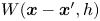 $W(\boldsymbol x-{\boldsymbol x}^\prime,h)$,
 $h$ is the smoothing length defining the influence domain of a particle. Some requirements or properties for the kernel function should be satisfied for a better performance, including the unity, compact support and positivity (for more details, see Liu & Liu Reference Liu and Liu2003, Reference Liu and Liu2010). Various kernel functions have been used in the literature, such as the Gaussian kernel (Gingold & Monaghan Reference Gingold and Monaghan1977), the cubic B-spline function (Monaghan & Lattanzio Reference Monaghan and Lattanzio1985), the higher-order (quartic and quintic) splines (Morris Reference Morris1996), and the Wenland function class (Wendland Reference Wendland1995). Among them, the Wendland C2 kernel is employed in this study due to its computational convenience and the capability to prevent pairing instability (Dehnen & Hossam Reference Dehnen and Hossam2012), which reads
 \begin{equation} W=\alpha_d\begin{cases} (1-q/2)^4(2q+1), & 0\leq{q}\leq2,\\ 0, & q>2, \end{cases} \end{equation}
where  $\alpha _d$ is a constant, taking the value
 ${7}/{(4{\rm \pi} h^2)}$ in two dimensions, and
 ${21}/{(16{\rm \pi} h^3)}$ in three dimensions, and
 $q=r/h$ is the non-dimensional distance between points
 $\boldsymbol x$ and
 $\boldsymbol x^\prime$, with
 $r=\| \boldsymbol x- \boldsymbol x^\prime \|$.
When the field function in (3.2) is replaced by its spatial derivative, we can get the following expression by using integration by parts:
 \begin{equation} \boldsymbol{\nabla}{f(\boldsymbol{x})} \doteq\int_{\varOmega}f(\boldsymbol{x}^{\prime})\,\boldsymbol{\nabla}_{\boldsymbol{x}}W(\boldsymbol{x}-\boldsymbol{x}^{\prime},h)\,{\rm d}\kern0.06em \boldsymbol x^\prime, \end{equation}
where  $\boldsymbol {\nabla }_{\boldsymbol {x}}$ represents the gradient with respect to
 $\boldsymbol x$. The kernel approximation of the diffusion term in (2.5) has the expression
 \begin{align} \boldsymbol{\nabla}(g(\boldsymbol x)\,\boldsymbol{\nabla} f(\boldsymbol x))=\int_{\varOmega}[g(\boldsymbol x)+g(\boldsymbol x^\prime)][\,f(\boldsymbol x)-f(\boldsymbol x^\prime)]\,\frac{\boldsymbol{x}-\boldsymbol{x}^{\prime}}{\| \boldsymbol{x}-\boldsymbol{x}^{\prime}\|^2}\boldsymbol{\cdot} \boldsymbol{\nabla}_{\boldsymbol{x}}W(\boldsymbol{x}-\boldsymbol{x}^{\prime},h)\,{\rm d}\kern0.06em \boldsymbol x^\prime. \end{align}
Details of the mathematical deduction of this equation are presented in Appendix D. Hitherto, we have constructed the integral representations of the field function, its derivative, and the diffusion term in the governing equations. The second step is to conduct the particle approximation, at which stage discrete particles will be used to replace the continuous domain, and the integral representations will be converted as summations over all the particles in the support domain such that
 $$\begin{gather} f(\boldsymbol{x}_i) \doteq\sum_{j=1}^{n}f(\boldsymbol{x}_j)\,W_{ij}m_j/\rho_j, \end{gather}$$
 $$\begin{gather}\boldsymbol{\nabla}{f(\boldsymbol{x}_i)} \doteq\sum_{j=1}^{n}f(\boldsymbol{x}_j)\,\boldsymbol{\nabla}_i{W_{ij}m_j}/\rho_j, \end{gather}$$
 $$\begin{gather}\{ \boldsymbol{\nabla}(g(\boldsymbol x)\,\boldsymbol{\nabla} f(\boldsymbol x))\} _i=\sum_{j=1}^{n}[g(\boldsymbol x_i)+g(\boldsymbol x_j)][\,f(\boldsymbol x_i)-f(\boldsymbol x_j)]\,\frac{\boldsymbol{x}_{ij}}{\| \boldsymbol{x}_{ij}\| ^2+\eta^2}\boldsymbol{\cdot}\boldsymbol{\nabla}_i{ W_{ij}}m_j/\rho_j, \end{gather}$$
where the subscripts  $i$ and
 $j$ denote the target particle and the neighbouring particles in the support domain;
 $n$ means the total particle number within the support domain of particle
 $i$;
 $\boldsymbol x_{ij}=\boldsymbol x_i-\boldsymbol x_j$;
 $\eta =0.1h$ acts as a clipping constant to keep the denominator non-zero;
 $W_{ij}$ is short for
 $W(\boldsymbol x_{ij},h)$; and
 $\boldsymbol {\nabla }_i{W_{ij}}$ short for
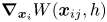 $\boldsymbol {\nabla }_{\boldsymbol {x}_i}W(\boldsymbol x_{ij},h)$.
3.2. The SPH discretization of governing equations
By applying (3.6)–(3.8), one can obtain the SPH formulation for the momentum conservation equation as
 \begin{equation} \frac{{\rm d}\boldsymbol u_i}{{\rm d}t}=\sum_{j=1}^{n}m_j\left( \frac{\boldsymbol\sigma_i}{\rho_i^2}+\frac{\boldsymbol\sigma_j}{\rho_j^2}+\varPi_{ij}\right)\boldsymbol{\nabla}_i W_{ij} +\boldsymbol g. \end{equation}
In (3.9),  $\varPi _{ij}$ denotes the artificial viscosity, which is a common stabilization scheme in the SPH theory to damp out unphysical numerical oscillations. In this study, the formulation proposed by Monaghan (Reference Monaghan1992) is adopted, reading
 \begin{equation} \varPi_{ij}=\begin{cases} \dfrac{\alpha_{\varPi}{c_{s}}h}{{\bar\rho}_{ij}}\,\dfrac{\boldsymbol{u}_{ij}\boldsymbol{\cdot}\boldsymbol{x}_{ij}}{\| \boldsymbol{x}_{ij}\| ^2+0.01h^2}, & \boldsymbol{u}_{ij}\boldsymbol{\cdot}\boldsymbol{x}_{ij}<0,\\ 0, & \boldsymbol{u}_{ij}\boldsymbol{\cdot}\boldsymbol{x}_{ij}\geq0, \end{cases} \end{equation}
in which  $\alpha _{\varPi }$ is a constant coefficient, taken as 0.1 in this study (Bui et al. Reference Bui, Fukagawa, Sako and Ohno2008);
 $c_{s}$ is the sound velocity;
 $\bar \rho _{ij}=0.5( \rho _i+\rho _j)$ is the average density of particles
 $i$ and
 $j$; and
 $\boldsymbol u_{ij}=\boldsymbol u_i-\boldsymbol u_j$. The specific terms related to stress in (3.9) come from the identity
 \begin{equation} \frac{\boldsymbol{\nabla}\boldsymbol\sigma}{\rho}=\boldsymbol{\nabla}\boldsymbol{\cdot}\left( \frac{\boldsymbol\sigma}{\rho}\right) +\frac{\boldsymbol\sigma}{\rho^2}\,\boldsymbol{\nabla}\rho. \end{equation}
The pairwise SPH form of the momentum equation, i.e. (3.9), ensures the action–reaction principle and is stable in the calculation, thus gaining high popularity. Note that SPH suffers from the short-length-scale-noise problem, which could lead to unrealistic stress perturbations (Nguyen et al. Reference Nguyen, Nguyen, Bui, Nguyen and Fukagawa2000; Monaghan Reference Monaghan2012). To regularize the stress field, the Shepard filter scheme is adopted every so many steps ( $N_{step} = 30$ in this study) to reproduce the linear variation of stress fields, reading
 \begin{equation} \sigma_i^{new}=\frac{\sum\sigma_jW_{ij}}{\sum W_{ij}}. \end{equation}
Likewise, the SPH formulation for the segregation–diffusion equation should be written as
 \begin{align} \frac{{\rm d}C}{{\rm d}t}&=-\sum_{j=1}^{n}\frac{m_j}{\rho_j}\,( V_i\mathcal{F}_{i}C_{ij}+F_{i}V_{ij})\,\frac{\boldsymbol g}{\| \boldsymbol g\|}\boldsymbol{\cdot}\boldsymbol{\nabla}_i W_{ij}\nonumber\\ &\quad +\sum_{j=1}^{n}\frac{m_j}{\rho_j}\,(D_i+D_j)C_{ij}\,\frac{\boldsymbol{x}_{ij}}{\| \boldsymbol{x}_{ij}\| ^2+\eta^2}\boldsymbol{\cdot}\boldsymbol{\nabla}_i{ W_{ij}}, \end{align}
where  $C_{ij}=C_i-C_j$ and
 $V_{ij}=V_i-V_j$. A similar process for the strain rate tensor and spin tensor gives
 $$\begin{gather} \dot{\boldsymbol\varepsilon}=\dfrac{1}{2}\left( \sum_{j=1}^{n}\boldsymbol u_{ij}\otimes\boldsymbol{\nabla}_i{W_{ij}m_j}/\rho_j+\sum_{j=1}^{n}\boldsymbol{\nabla}_i{W_{ij}}\otimes\boldsymbol u_{ij}m_j/\rho_j\right) \!, \end{gather}$$
 $$\begin{gather}\dot{\boldsymbol \omega}=\dfrac{1}{2}\left( \sum_{j=1}^{n}\boldsymbol u_{ij}\otimes\boldsymbol{\nabla}_i{W_{ij}m_j}/\rho_j-\sum_{j=1}^{n}\boldsymbol{\nabla}_i{W_{ij}}\otimes\boldsymbol u_{ij}m_j/\rho_j\right) \!, \end{gather}$$
where  $\boldsymbol u_{ij}=\boldsymbol u_i-\boldsymbol u_j$. The inclusion of
 $\boldsymbol u_i$ is because of the identity
 \begin{equation} \sum_{j=1}^{n}\boldsymbol u_{i}\otimes\boldsymbol{\nabla}_i{W_{ij}m_j}/\rho_j=\boldsymbol 0. \end{equation}
One benefit of the adoption of the velocity difference  $\boldsymbol u_{ij}$ in (3.14)–(3.15) is the restoration of
 $O(h)$ convergence on the free surface (Colagrossi, Antuono & Le Touzé Reference Colagrossi, Antuono and Le Touzé2009).
3.3. Time stepping
The SPH forms of the governing equations are solved numerically using explicit time integration schemes. In this work, we employ a second-order predictor–corrector integrator (Zhu et al. Reference Zhu, Peng and Wu2022a). At the predictor step, the physical variables at the midpoint of the calculation step are evaluated with
 \begin{equation} X^{n+0.5}=X^n+\varGamma^{n}\,\Delta t, \end{equation}
in which  $X$ goes through position
 $\boldsymbol x$, velocity
 $\boldsymbol v$, stress
 $\boldsymbol \sigma$ and concentration
 $C$, and
 $\varGamma ={\rm d}X/{\rm d}t$ is the material time derivative of
 $X$. At the corrector step, the final value at the end of the calculation step is obtained with
 \begin{equation} X^{n+1}=X^n+\varGamma^{n+0.5}\,\Delta t. \end{equation}
Here,  $\varGamma ^{n+0.5}$ is determined with
 $X^{n+0.5}$ from the predictor step. Note that the time step
 $\Delta t$ used in the time integration is limited by the CFL condition
 \begin{equation} \Delta{t}=\chi_{CFL}\times\min \left(\sqrt{h/a_{max}},\frac{h}{c_s}\right)\!, \end{equation}
where  $\chi _{CFL}$ is the CFL coefficient, taken as 0.1 in this study, and
 $a_{max}$ denotes the maximum acceleration among all material particles.
3.4. Numerical implementations
The proposed SPH model is developed based on our in-house code LOQUAT, an open-source SPH solver (Peng et al. Reference Peng, Wang, Wu, Yu, Wang and Chen2019). In each calculation step, four subroutines are executed serially, including (1) nearest neighbouring particle searching, (2) boundary treatment, (3) particle interaction, and (4) time integration. Boundary treatment refers to the fulfilment of specific boundary conditions, which will be illustrated in detail in § 4. Particle interaction in this work means that the SPH approximation of the material time derivative of velocity and concentration from the support domain, i.e. (3.9) and (3.13). The introduction to time integration was presented in the previous subsection. Here, we focus mainly on the illustration of the first subroutine.
An SPH particle interacts only with its nearest neighbouring particles (NNP) located within the influence domain, so the prerequisite of SPH computations is identifying these particles. This process is referred to as nearest neighbouring particle searching (NNPS) in the literature. A naive strategy is to conduct the calculation of all pairwise distances between particles  $i$ and
 $j$. Particle
 $j$ is found to belong to the support domain of particle
 $i$ provided that the distance is less than
 $2h$. However, this method would be prohibitively expensive for large-scale problems, as the computational burden of such an operation is of order
 $O(N^2)$. Therefore, various alternatives have been proposed to improve search efficiency. Typical examples include the Verlet neighbour list, cell-linked list and tree searching algorithms (Liu & Liu Reference Liu and Liu2003; Viccione, Bovolin & Carratelli Reference Viccione, Bovolin and Carratelli2008).
Among all the approaches, this study adopts the cell-linked list scheme to advance NNPS. The first step in implementing this algorithm is to cover the whole calculation domain with a virtual square lattice mesh whose length is equal to  $2h$, as shown in figure 3. Each cell is indexed by
 $\alpha$,
 $\beta$ and
 $\gamma$ according to its position. With this background grid, all SPH particles can be binned into the corresponding cells. From figure 3, we can find that the support domain is encircled by the neighbour cells so that NNPS can be confined to the
 $M$ particles from these cells. As a result, the neighbour search operation is scaled down to the order
 $O(MN)$. The cell-linked list scheme needs to store all particles in each cell, which is memory-consuming. Green (Reference Green2010) proposed a modification by sorting all the particles according to their associated cell index, thus only the beginning and ending particle indexes are necessary for each cell. This modified cell-linked list not only consumes less memory, but also has a high data accessing rate since all information is stockpiled in memory serially.
Sketch of the virtual square lattice mesh.

4. Boundary conditions
4.1. Kinematic and dynamic boundary condition
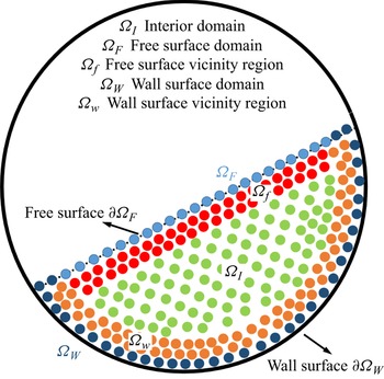
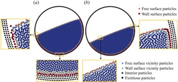
A proper formulation of boundary conditions for SPH is crucially important to achieve physically meaningful and quantitatively correct results (Adami, Hu & Adams Reference Adami, Hu and Adams2012). However, the implementation of boundary conditions in SPH is far from trivial and is often regarded as a major weakness compared to the FEM, thus identified as one of the grand challenges (Vacondio et al. Reference Vacondio, Altomare, De Leffe, Hu, Le Touzé, Lind, Marongiu, Marrone, Rogers and Souto-Iglesias2021). For instance, in a rotating drum, two boundary conditions are concerned, i.e. a free surface and rigid wall boundary, as shown in figure 4. One distinct advantage of the SPH method is the intrinsic fulfilment of the kinematic and dynamic boundary conditions on the free surfaces (Colagrossi et al. Reference Colagrossi, Antuono and Le Touzé2009; Lyu & Sun Reference Lyu and Sun2022).
Sketch of a granular flow with a free surface and rigid wall boundary.

On the rigid wall boundaries, the dummy particle scheme, initially proposed for fluid flow (Adami et al. Reference Adami, Hu and Adams2012), and later modified for geomaterials (Peng et al. Reference Peng, Wang, Wu, Yu, Wang and Chen2019; Zhan et al. Reference Zhan, Peng, Zhang and Wu2019; Zhu et al. Reference Zhu, Peng, Wu and Wang2022b), is employed for modelling the rigid wall boundary due to its accuracy and efficiency for regular boundary geometries (Valizadeh & Monaghan Reference Valizadeh and Monaghan2015). As shown in figure 5, at the beginning of the simulation, several layers of dummy particles (depending on the ratio of smoothing length to the initial particle spacing, i.e.  $h/\Delta r$) are arranged outside the calculation domain. The fictitious particles participate in the interaction if they are located in the support domain of the material particles. However, unlike the internal particles, whose field variables are updated according to the governing equations, the necessary information of the dummy particles is extrapolated from those material particles close to the boundary (named boundary particles, hereafter). For a non-slip boundary condition, the following extrapolation scheme is applied:
 \begin{equation} \boldsymbol u_d=2\boldsymbol u_w-\frac{\displaystyle\sum_{m=1}^{n}\boldsymbol u_mW_{dm}V_m}{\displaystyle\sum_{m=1}^{n}W_{dm}V_m}, \end{equation}
where the subscripts  $d$ and
 $m$ refer to dummy and material, respectively, and
 $\boldsymbol u_w$ represents the prescribed velocity of the rigid wall. In the scenario of a free-slip boundary, the procedure remains the same with (4.1) for the normal component of the velocity vector, while the tangential part is modified as follows:
 \begin{equation} \left.\begin{array}{c} u_d^{n}=2 u_w^{n}-\dfrac{\displaystyle\sum_{m=1}^{n} u_m^{n}W_{dm}V_m}{\displaystyle\sum_{m=1}^{n}W_{dm}V_m},\\ u_d^\tau=\dfrac{\displaystyle\sum_{m=1}^{n} u_m^{\tau}W_{dm}V_m}{\displaystyle\sum_{m=1}^{n}W_{dm}V_m}, \end{array}\right\} \end{equation}
where the superscripts  $n$ and
 $\tau$ represent the normal and tangential directions. To avoid the particle penetration through the rigid wall, the dummy particles are assigned the following stress (Adami et al. Reference Adami, Hu and Adams2012; Peng et al. Reference Peng, Wang, Wu, Yu, Wang and Chen2019):
 \begin{equation} \boldsymbol \sigma_d = \dfrac{\displaystyle\sum_{m=1}^{n}\boldsymbol\sigma_mW_{dm}V_m+\boldsymbol{\mathsf{I}} \circ\sum_{m=1}^{n}m_m\boldsymbol g\otimes\boldsymbol r_{dm}W_{dm}}{\displaystyle\sum_{j=1}^{n}W_{dm}V_m}, \end{equation}
in which  $\circ$ denotes the Hadamard product, and
 $\boldsymbol r_{dm}=\boldsymbol r_d - \boldsymbol r_m$.
Dummy particle scheme for the rigid wall boundary.

4.2. Inhomogeneous Neumann boundary condition
The above section presents the procedure for achieving the kinematic and dynamic boundary conditions. We proceed to show strategies on how to realize the concentration-related boundary conditions.
Provided that there is no concentration flux of small particles across the boundary, the mathematical expression can be written as follows (Gray & Chugunov Reference Gray and Chugunov2006):
 \begin{equation} \boldsymbol n \boldsymbol{\cdot} \left(Q\,\dfrac{\boldsymbol g}{\| \boldsymbol g\| }+D\,\boldsymbol{\nabla} C\right)=0,\quad \forall \boldsymbol x \in \partial\varOmega, \end{equation}
in which  $\boldsymbol n$ denotes the normal vector on
 $\partial \varOmega$ pointing towards
 $\varOmega$. Equation (4.4) reveals that the segregation and diffusion fluxes have identical magnitude but opposite direction along the normal of the boundary. After some mathematical manipulations, an inhomogeneous Neumann boundary condition about
 $C$ can be reached as follows:
 \begin{equation} D\,\dfrac{\partial C}{\partial \boldsymbol n}=f(C)=-VF\,\dfrac{\boldsymbol n \boldsymbol{\cdot} \boldsymbol g}{\| \boldsymbol g\| },\quad \forall \boldsymbol x \in \partial\varOmega. \end{equation}
Here,  $V$ and
 $F$ denote the segregation velocity and segregation functions (cf. (2.6)).
4.2.1. Continuum surface reaction scheme for solid boundaries
It is challenging to enforce the inhomogeneous Neumann boundary condition within the SPH framework directly. Following the spirit of the continuum surface reaction (CSR) method (Ryan, Tartakovsky & Amon Reference Ryan, Tartakovsky and Amon2010), the inhomogeneous Neumann boundary condition can be replaced by the homogeneous Neumann boundary condition and a volumetric source term added into the segregation–diffusion equation (Wang et al. Reference Wang, Hu, Zhang and Pan2019), reading
 $$\begin{gather} \dfrac{\partial C}{\partial \boldsymbol n}=0,\quad \forall \boldsymbol x \in \partial\varOmega, \end{gather}$$
 $$\begin{gather}\dfrac{{\rm d}C}{{\rm d}t}=-V\mathcal{F}\,\boldsymbol{\nabla}_{g}C-F\,\boldsymbol{\nabla}_{g}V+\boldsymbol{\nabla}(D\,\boldsymbol{\nabla} C )+q. \end{gather}$$
The implementation of the homogeneous Neumann boundary condition in SPH can be enforced by assuming that the virtual and concerned material particles have identical concentrations, i.e.  $C_j=C_i$ (Wang et al. Reference Wang, Hu, Zhang and Pan2019), which is achieved intrinsically with the SPH form of the Laplace operator adopted in (3.13). The last term on the right-hand side of (4.7), i.e.
 $q$, is the volumetric source term, which is related to
 $f(C)$ through the expression
 \begin{equation} q=- f( C)\int_{\varOmega_{s}}[\boldsymbol n(\boldsymbol x)+\boldsymbol n(\boldsymbol x^\prime)]\boldsymbol{\cdot}\boldsymbol{\nabla}_{\boldsymbol{x}}W(\boldsymbol x-\boldsymbol x^\prime,h)\,{\rm d}\kern0.06em \boldsymbol x^\prime, \end{equation}
where the integral domain  $\varOmega _{s}$ (as seen in figure 5) denotes the missing support truncated by the boundary. The SPH approximation to (4.8) is
 \begin{equation} q_{i}=-f( C_i)\sum_{j\in\varOmega_{s}}(\boldsymbol n_i+\boldsymbol n_j)\,\boldsymbol{\nabla}_iW_{ij}V_j. \end{equation}
Here, the normal vectors at points  $i$ and
 $j$, i.e.
 $\boldsymbol n_i$ and
 $\boldsymbol n_j$, are evaluated with
 \begin{equation} \boldsymbol n_i=\dfrac{\displaystyle\sum_{j\in\varOmega\cup\varOmega_{s}}(c_i-c_j)\,\boldsymbol{\nabla}_iW_{ij}V_j}{\left| \displaystyle\sum_{j\in\varOmega\cup\varOmega_{s}}(c_i-c_j)\,\boldsymbol{\nabla}_iW_{ij}V_j\right| }, \end{equation}
where  $c$ represents a colour function whose value is 0 for the material particles, and 1 for the fictitious particles. However, the CSR scheme introduced above is found only with first-order accuracy, thus errors could arise near the boundary (Pan et al. Reference Pan, Kim, Perego, Tartakovsky and Parks2017). To remedy this, a degenerate function
 $\psi _d$ is introduced, and the segregation–diffusion equation is modified as (Wang et al. Reference Wang, Hu, Zhang and Pan2019)
 \begin{equation} \dfrac{{\rm d}C}{{\rm d}t}=-V\mathcal{F}\,\boldsymbol{\nabla}_{g}C-F\,\boldsymbol{\nabla}_{g}V+\boldsymbol{\nabla}(\psi_dD\,\boldsymbol{\nabla} C )+q, \end{equation}
where  $\psi _d$ can be specified with
 \begin{equation} \psi_d(\boldsymbol x)=\begin{cases} 1, & \boldsymbol x\in\varOmega,\\ 0, & \boldsymbol x\in\partial\varOmega,\\ -1, & \boldsymbol x\in\varOmega_{s}. \end{cases} \end{equation}
The corresponding SPH form of the Laplace operator in (4.11) can be given as
 \begin{equation} {\boldsymbol{\nabla}(\psi_dD\,\boldsymbol{\nabla} C )}=\sum_{j=1}^{n}\dfrac{m_j}{\rho_j}\,(\tilde\psi_{di}D_i+\tilde\psi_{dj}D_j)C_{ij}\,\dfrac{\boldsymbol{x}_{ij}}{\| \boldsymbol{x}_{ij}\| ^2+\eta^2}\boldsymbol{\cdot}\boldsymbol{\nabla}_i{ W_{ij}}, \end{equation}
where  $\tilde \psi _{d}$ represents the smoothed counterpart of
 $\psi _{d}$, defined as
 \begin{equation} \tilde\psi_{di}=\dfrac{\displaystyle\sum_{j\in\varOmega\cup\varOmega_{s}}\psi_{dj}W_{ij}V_j}{\displaystyle\sum_{j\in\varOmega\cup\varOmega_{s}}W_{ij}V_j}. \end{equation}
4.2.2. Hybrid CSR scheme
The conventional CSR (CCSR) scheme introduced above evaluates physical fields based on the missing support domain, e.g. (4.9) and (4.10). This can be achieved trivially on the rigid wall boundary, i.e.  $\partial \varOmega _{W}$, where the missing support domain is supplemented by the fictitious particles. However, the implementation on the dynamic free surface will be troublesome, particularly when the geometry is irregular. To fulfil (4.6) on the free surface, we put forward a modified CSR (MCSR) scheme that can avoid introducing additional fictitious particles because the SPH approximation to the volumetric source term (
 $q$) and degenerate function (
 $\tilde \psi _{d}$) is carried out using the material particles.
This new variant has the same boundary condition and governing equation as (4.6) and (4.11), but with the following kernel approximation to the volumetric source term:
 \begin{equation} q=2\,f( C)\,\boldsymbol n(\boldsymbol x)\boldsymbol{\cdot}\int_{\varOmega}\boldsymbol{\nabla}_{\boldsymbol{x}}W(\boldsymbol x-\boldsymbol x^\prime,h)\,{\rm d}\kern0.06em \boldsymbol x^\prime. \end{equation}
Correspondingly, the SPH approximation to  $q$ is
 \begin{equation} q_{i}=2\,f( C_i)\sum_{j\in\varOmega}\boldsymbol n_i\,\boldsymbol{\nabla}_iW_{ij}V_j. \end{equation}
Here,  $\boldsymbol n_i$ is evaluated with
 \begin{equation} \boldsymbol
n_i=\begin{cases}
\dfrac{\displaystyle\sum_{j\in\varOmega}\boldsymbol{\nabla}_iW_{ij}V_j}{\displaystyle\left|
\sum_{j\in\varOmega}\boldsymbol{\nabla}_iW_{ij}V_j\right|},
& i\in\varOmega_{F},\\
\dfrac{\displaystyle\sum_{j\in\varOmega_{F}}\boldsymbol{\nabla}_iW_{ij}V_j}{\displaystyle\left|
\sum_{j\in\varOmega_{F}}\boldsymbol{\nabla}_iW_{ij}V_j\right|
}, & i\in\varOmega_{f}. \end{cases}
\end{equation}
In this equation,  $\varOmega _{F}$ denotes the subset consisting of free surface particles, and
 $\varOmega _{f}$ indicates the particles in the vicinity of the free surface, as shown in figure 4. The procedure to identify these particles will now be presented. The smoothed degenerate function has the expression
 \begin{equation} \tilde\psi_{di}=2\sum_{j\in\varOmega}W_{ij}V_j-1. \end{equation}
Note that the volumetric source term should vanish (i.e.  $q_{i}=0$) for the material particles with full support domain (i.e.
 $\varOmega _{I}$ in figure 4). This is satisfied intrinsically within the CCSR scheme as the approximation to
 $q$ is based on the fictitious particles. However, the MCSR scheme employs the material particles, so non-zero value always appears due to the distorted particle distribution, especially for a granular flow with large deformation. One effective strategy to mitigate this issue is to restrict the MCSR scheme to only those material particles in the vicinity of the free surface (i.e.
 $\varOmega _{F}$ and
 $\varOmega _{f}$ in figure 4). To achieve this, the following boundary particle searching algorithm is proposed.
Step 1, identifying the surface particles (i.e.  $\varOmega _{F}$,
 $\varOmega _{W}$ in figure 4). In this step, the surface detection scheme proposed by Marrone et al. (Reference Marrone, Colagrossi, Le Touzé and Graziani2010) is adopted with some optimization. In the optimized version, a rough-refining two-stage strategy is used to advance the searching. First, those non-empty virtual cells are divided into three categories. Type I is the outermost layer, featured with some empty neighbour cells. Type II is the second outermost layer, which are intermediate neighbour cells of Type I. The remaining cells, i.e. the interior ones, consist of Type III. Since the lattice mesh has length
 $2h$, we can conclude that all the particles located in Type I cells could have truncated support. In comparison, particles in Type III cells have complete support. In this manner, Type II cells can be regarded as transitional regions, as some particles in Type II cells will have full support in
 $\varOmega$, while the rest do not. Accordingly, we can reduce the further searching in the next stage to only those particles from Type I cells. Subsequently, the surface particles are detected from the potential candidates by searching the so-called ‘umbrella-shaped’ region, as sketched in figure 6. A concerned particle will be considered as a surface particle if the ‘umbrella-shaped’ region is particle-free, i.e.
 \begin{equation} \left.\begin{array}{c@{}} \nexists \,j\in\{ \boldsymbol x_j\,|\, |\boldsymbol x_{ij}|\geq\sqrt{2}h \text{ and } |\boldsymbol x_{jT}|< h \},\\ \nexists \,j\in\left\{ \boldsymbol x_j\,|\,|\boldsymbol x_{ij}|<\sqrt{2}h \text{ and } \boldsymbol x_{ij} \boldsymbol{\cdot}\boldsymbol x_{iT} >\dfrac{\sqrt{2}}{2}\,|\boldsymbol x_{ij} |\,h \right\}. \end{array}\right\} \end{equation}
Sketch of the boundary particle detection scheme.

Step 2, determining the surface vicinity particles (i.e.  $\varOmega _f$,
 $\varOmega _w$ in figure 4). One can observe from figure 6 that the surface vicinity particles come from Type I or II cells, thus the searching operation is also of a small amount compared to the total SPH particle number. In this work, an SPH particle is considered a free-surface vicinity particle (i.e.
 $\boldsymbol x_i\in \varOmega _{f}$) when the following condition is satisfied:
 \begin{equation} \min\{ | \boldsymbol x_{ij}| \,|\,\boldsymbol x_j\in\varOmega_{F}\} < 2h-\Delta r. \end{equation}
The identification of  $\varOmega _{w}$ is based on its definition, i.e.
 \begin{equation} \varOmega_{w}:=\{ \boldsymbol x_i\,|\,\exists \boldsymbol x_j \in\varOmega_{s}, \text{ but }\boldsymbol x_i \notin\varOmega_{W}\}. \end{equation}
In practice, CCSR is used for particles in domains  $\varOmega _{W}$ and
 $\varOmega _{w}$, while MCSR is used for those in domains
 $\varOmega _{F}$ and
 $\varOmega _{f}$. This implementation scheme is named the hybrid continuum surface reaction (HCSR) method in this study. Note that the identification of
 $\varOmega _{W}$ and
 $\varOmega _{w}$ is unnecessary within the framework of CCSR, but indispensable for obtaining accurate segregation flux at the boundary
 $\partial \varOmega$, which will be introduced in the next subsection for the whole boundary particles.
4.3. Accurate approximation to the segregation flux gradient
The SPH approximation of the segregation flux gradient adopted in (3.13) has  $C^1$ consistency at the interior particles, but this level of accuracy is infeasible at the boundary particles due to the particle deficiency. The mirroring technique with antisymmetric extension of
 $C$ and
 $V$ can restore the
 $C^1$ consistency close to the boundaries (Macia et al. Reference Macia, Antuono, González and Colagrossi2011). However, this method needs to introduce virtual particles around the boundary
 $\partial \varOmega$, which is difficult for implementation when the boundary has an irregular shape, as discussed earlier. In this study, we employ the approach proposed by Liu & Liu (Reference Liu and Liu2011) to obtain the accurate approximation with
 $C^1$ consistency for
 $\boldsymbol {\nabla }_{g}C$ and
 $\boldsymbol {\nabla }_{g}V$ in (2.10). Details can be found in Appendix B. This method needs only the information from material particles, thus avoiding introduction of fictitious particles. Note that this technique is restricted to boundary particles (
 $\varOmega -\varOmega _{I}$). For the interior particles (
 $\varOmega _{I}$), the standard SPH approximation, i.e. (3.13), is used for obtaining the segregation flux gradient.
5. Validation
Van der Vaart et al. (Reference Van der Vaart, Gajjar, Épely-Chauvin, Andreini, Gray and Ancey2015) investigated experimentally the particle segregation in a shear box that was 51 mm deep, 37 mm wide, and filled with bidisperse glass beads to height  $H=87\pm 3$ mm, as shown in figure 7. In the initial configuration, the lower half are large beads with diameter
 $d^{L}=8$ mm, underlying the small beads with
 $d^{S}=4$ mm. The side walls oscillate at a consistent pace with periodic shear
 $\gamma (t)=\gamma _0\sin (\omega t)$ and period
 $T=13$ s, thus remaining parallel all the time. The maximum inclination of the side wall throughout the experiment is
 $\pm 30^\circ$, giving a maximum grain displacement amplitude
 $B=H\gamma _0$. This benchmark, which can be modelled as a one-, two- or three-dimensional problem, is an excellent choice for examining the proposed SPH model. In this section, we conduct a two-dimensional simulation with the prescribed velocity to validate the effectiveness of the proposed HCSR scheme and the capability of the SPH method to reproduce the particle segregation evolution.
Experimental set-up of the shear box in Van der Vaart et al. (Reference Van der Vaart, Gajjar, Épely-Chauvin, Andreini, Gray and Ancey2015).

The concentration of the small grains is initialized as
 \begin{equation} C(0,z)=\begin{cases} 0, & 0\le z/H\le 0.5,\\ 1, & 0.5< z/H\le 1. \end{cases} \end{equation}
Also, (4.6) is applied to all boundaries. Note that the previous numerical studies prefer to adopt the constant segregation velocity and diffusivity rather than the functional forms (Van der Vaart et al. Reference Van der Vaart, Gajjar, Épely-Chauvin, Andreini, Gray and Ancey2015; Yang et al. Reference Yang, Zheng, Bai and Yu2021). In this study, both the constant and functional forms of  $V$ and
 $D$ are adopted to demonstrate the capability of the developed numerical method.
5.1. Constant segregation velocity and diffusivity
In this subsection, both segregation velocity and diffusivity are assumed constant, following the practice in Van der Vaart et al. (Reference Van der Vaart, Gajjar, Épely-Chauvin, Andreini, Gray and Ancey2015). The obtained concentration distributions at various time instants are compared with experimental observations from Van der Vaart et al. (Reference Van der Vaart, Gajjar, Épely-Chauvin, Andreini, Gray and Ancey2015), and the numerical prediction using the pdepe routine of MATLAB subject to the same initial and boundary conditions. In MATLAB calculation, this problem is simplified as a one-dimensional problem with (2.5) as the governing equation, and the domain is discretized with 201 nodes. Here, we regard the MATLAB calculation result as a first-principles benchmark. Consistent with Van der Vaart et al. (Reference Van der Vaart, Gajjar, Épely-Chauvin, Andreini, Gray and Ancey2015), the geometry and time are normalized by the height  $H$ and the period
 $T$, respectively. A series of tests shows that the best agreement between the segregation time (the critical time to reach steady state) and the initial small-particle concentration is obtained with the following constant non-dimensional segregation velocity and diffusivity (Van der Vaart et al. Reference Van der Vaart, Gajjar, Épely-Chauvin, Andreini, Gray and Ancey2015):
 \begin{equation} \left.\begin{aligned} {[V]}^{const}&=V^{const}T/B=3.0\times10^{-2},\\ {[D]}^{const}&=D^{const}T/B^2=1.01\times10^{-3}. \end{aligned}\right\} \end{equation}
Therefore, these values are applied in this study.
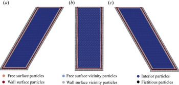
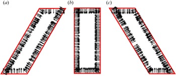
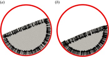
The physical model in SPH simulation is partitioned with  $\Delta r=0.01H$, which accounts for 4000 material particles and 858 fictitious particles. We first examine the performance of the HCSR method on the boundary particle searching and the normal direction identification, which is presented in figures 8 and 9. It is found that the boundary particles are identified accurately and classified at all three typical time instants. Also, the majority of the normal vectors are perpendicular to the boundaries, as expected. The satisfactory behaviour of the HCSR method indicates its capability in the boundary treatment, and gives us confidence in further segregation analysis.
Boundary particle identification in the HCSR method at (a)  $t/T = 0.25$, (b)
 $t/T = 0$ or 0.5, and (c)
 $t/T = 0.75$.

Normal direction on the boundary particles at (a)  $t/T = 0.25$, (b)
 $t/T = 0.5$ or 1.0, and (c)
 $t/T = 0.75$.

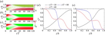
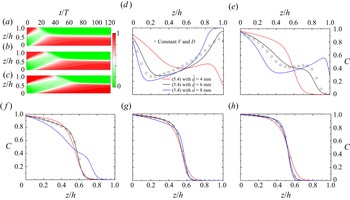
The experimental results show that the small beads migrate faster than the large ones, as seen by the asymmetric vertical distribution of the concentration  $C$ for the first 20 periods in figure 10(a). The symmetric segregation flux fails to reproduce this feature, which is, however, well captured by the asymmetric scheme (figures 10b,c). As the segregation continues, a relatively homogeneous mixture is found between
 $t/T=20$ and
 $t/T=40$. Afterwards, a reversed distribution pattern of
 $C$ starts to evolve, i.e. small beads are enriched at the bottom, compared to large ones at the top of the granular assembly. Finally, an equilibrium state is reached under the common effect of gravity-driven segregation and diffusion-induced remixing after
 $t/T=60$. Figures 10(d,e) present close agreement between the SPH prediction and MATLAB calculation at three specific time instants for both segregation flux schemes. All curves in figure 10(d) pass through and are symmetric about the centre point
 $(z/H, C)=(0.5,0.5)$. In comparison, relatively irregular patterns are observed in figure 10(e) with asymmetric segregation flux. The good consistency between the SPH prediction and the experimental observation as well as the MATLAB calculation result demonstrates the capability of the proposed SPH model, particularly the effectiveness of the HCSR method on boundary condition treatment.
Temporal evolution of the concentration of small glass beads. (a) Experimental observation from Van der Vaart et al. (Reference Van der Vaart, Gajjar, Épely-Chauvin, Andreini, Gray and Ancey2015). (b,c) The SPH predictions with symmetric and asymmetric segregation flux, respectively. (d,e) Vertical distributions of concentration  $C$ at three specific time instants from SPH prediction (lines) and MATLAB solution (symbols) with symmetric and asymmetric segregation flux.

The convergence performance is another key concern for a newly developed solver. Figure 11 presents the concentration distribution at  $t/T=80$ in the case of asymmetric segregation flux with four resolution levels (
 $\Delta r/H = 0.005$, 0.01, 0.02 and 0.04). Good agreement is observed between MATLAB calculation and the numerical predictions for all resolution levels. Even the coarsest partition scheme, i.e.
 $\Delta r=0.04 H$, with only 25 material particles in the height direction, gives a reasonable prediction. Furthermore, as the partition becomes finer, the SPH prediction converges rapidly to the MATLAB calculation result. The convergence property of the proposed SPH method can be observed quantitatively from the values of the mean absolute error (MAE) and root mean square error (RMSE) with the following expressions:
 $$\begin{gather} \text{MAE}=\dfrac{\displaystyle\sum_{i=1}^{n}|C_i^{SPH}-C_i^{MATLAB}|}{n}, \end{gather}$$
 $$\begin{gather}\text{RMSE}=\sqrt{\dfrac{\displaystyle\sum_{i=1}^{n}( C_i^{SPH}-C_i^{MATLAB})^2 }{n}}. \end{gather}$$
Both MAE and RMSE of the concentration error against the MATLAB results are plotted in figure 12, with satisfactory order of convergence 1.25.
Consistency test for the proposed SPH method with the MATLAB pdepe calculation result as benchmark. Curves represent the concentration distribution at  $t/T=80$ with the asymmetric segregation flux scheme.

The error of concentration at  $t/T=80$.

5.2. Varying segregation velocity and diffusivity
In this subsection, the functional forms of segregation velocity  $[ V]$ and diffusivity
 $[ D]$ will be employed to demonstrate the capability of the developed SPH model. To do this,
 $[{D}]$ and
 $[ {V}]$ in this subsection are assumed to have the following expressions:
 \begin{equation} [D] =\dfrac{\dot\gamma}{\dot\gamma_{m}}\left( \dfrac{d_{avg}}{\bar{d}}\right) ^2[D]^{const} ,\quad [V] =\dfrac{\dot\gamma}{\dot\gamma_{m}}\,\dfrac{d_{avg}}{\bar{d}}\,[ V]^{const}, \end{equation}
where 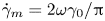 $\dot \gamma _{m}=2\omega \gamma _0/{\rm \pi}$ denotes the shear rate averaged over one complete cycle;
 $\bar {d}= (d^{S}+d^{L})/2$ is introduced for non-dimensionalization, and its effect on the simulation result will be discussed;
 $[D]^{const}=1.01\times 10^{-3}$ and
 $[ V] ^{const}=3.0\times 10^{-2}$ are kept the same as in the previous subsection. Substituting (2.7a,b) into (5.5a,b), the specific expressions and values of
 $\chi _{D}$ and
 $\chi _{V}$ can be derived as
 \begin{equation} \chi_{D} =\dfrac{B^2[D] ^{const}}{T\dot\gamma_{m}{\bar d}^2}=0.0307,\quad \chi_{V} =\dfrac{B[V]^{const} }{T\dot\gamma_{m}{\bar d}}=0.11. \end{equation}
The value of  $\chi _{D}$ obtained here is comparable with previous reports (for instance,
 $\chi _{D}\approx 0.053$ in Bridgwater (Reference Bridgwater1980),
 $\chi _{D}\approx 0.022$ in Hsiau & Shieh (Reference Hsiau and Shieh1999), and
 $\chi _{D}\approx 0.042$ in Fry et al. (Reference Fry, Umbanhowar, Ottino and Lueptow2019)). Substituting
 $\chi _{V} =0.11$ into (5.5a,b) leads to
 \begin{equation} V=0.11\dot\gamma d_{avg}=0.11\sim0.22\dot\gamma d_{S}, \end{equation}
which is in line with the experimental observation (Schlick et al. Reference Schlick, Fan, Isner, Umbanhowar, Ottino and Lueptow2015a)
 \begin{equation} V=0.26\dot\gamma d^{S} \log\left( \dfrac{d^{L}}{d^{S}}\right). \end{equation}
The initial conditions are aligned with (5.1), and the whole domain is discretized with  $\Delta r=0.01H$.
The temporal evolution of particle-size segregation in the shear cell is presented in figure 13, which shows the concentration distributions for both the whole duration and five typical time instants. Also, three cases with different  $\bar {d}$ values are reproduced numerically, namely,
 $\bar {d}=d^{S}$,
 $( d^{S}+d^{L})/2$ and
 $d^{L}$. From figure 13, it is observed clearly that with a greater
 $\bar {d}$, the particle segregation develops at a much slower pace. For instance, the cases with
 $\bar {d}$ from the smallest to the greatest reach the equilibrium state after approximately 40, 60 and 80 periods, respectively. This feature could also be verified from the concentration distributions in figures 13(d–f). Despite the fastest segregation evolution, it is found that the numerical simulation with
 $\bar d=4$ mm has the most pronounced discrepancy to the complete inverse grading at the equilibrium state, as shown by the slope of the curves at the mid-height of the shear cell in figure 13(h). Moreover, when comparing figures 13(a–c) to the temporal development of small-particle concentration from the experiment, i.e. figure 10(a), we find that numerical prediction with intermediate value
 $\bar d=6$ mm has the best match among all three cases. Furthermore, this value also generates the result with an approaching agreement to the numerical simulation with constant
 $[ V]$ and
 $[ D]$.
SPH predictions of the shear cell experiment with functional forms of segregation velocity  $V$ and diffusivity
 $D$: (a–c)
 $\bar d=4$, 6, 8 mm; (d–h) concentration distribution along the height at
 $t/T=20$, 40, 60, 80, 120.

The above findings indicate the significance of the parameters  $[ D]$ and
 $[ V]$ on the particle segregation evolution. On one hand, the segregation velocity
 $[ V]$ with a smaller
 $\bar d$ would be greater, and the particle segregation would evolve at a faster pace as a result. On the other hand, the concentration distribution at the steady state is determined by the ratio between the non-dimensional segregation velocity and diffusivity, i.e. the Péclet number, such that
 \begin{equation} Pe=\dfrac{[V] }{[D] }=\dfrac{\bar d[V] ^{const}}{d_{avg}[D] ^{const}}. \end{equation}
This equation implies a stronger segregation relative to the diffusion at the steady state with a greater  $\bar d$, which explains the concentration distribution in figure 13(h).
Figure 14 shows the time series of the depth-averaged concentration of small particles from theoretical calculation, experimental data and numerical simulations. In this case, the upper and lower halves of the column are filled with large and small particles, respectively, thus leading to the initial depth-averaged concentration equal to 0.5. Theoretically, this value should be constant throughout the numerical simulation as the granular material is assumed incompressible here, as shown by the scatters in figure 14. The experimental data are quite close to the theoretical values except for a maximum relative error of approximately 10 $\,\%$ showing up at
 $t=20 T$, which could be due to the measurement error from the refractive index matched fluid technique (Trewhela et al. Reference Trewhela, Ancey and Gray2021a). In comparison, good agreement is observed between the theoretical value and the results from SPH simulations for all four cases. This satisfactory match examines solidly the effectiveness of the proposed HCSR scheme in realizing the inhomogeneous Neumann boundary condition.
Temporal evolution of the depth-averaged concentration of small particles.

6. Application
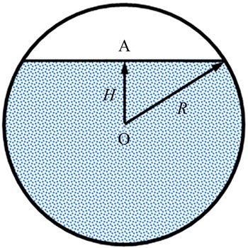
A rotating drum is a widely used facility in various walks of industry, such as the chemistry sector, food processing and building engineering. In this section, the proposed SPH model is applied to simulate the granular segregation of a size-bidisperse aggregate in a rotating drum, whose initial set-up is illustrated in figure 15. Here, the filling level is  $R_f$, which is defined as the ratio of the initial filling depth of the granular bed to the drum diameter, i.e.
 $(H+R)/2R$, with
 $R$ the radius and
 $H$ the distance from the drum centre (point O) to the free surface (point A) – positive when A is above O, otherwise negative. Table 1 lists the necessary parameters for the numerical simulation. Two configurations – that is, equal volume (EV) and equal number (EN) for small and large grains – are considered in the simulation. The filling levels are
 $59.1\,\%$ and
 $42\,\%$ in the case of EN and EV, respectively, while the rotating speed
 $\omega =5$ rpm is kept the same. This problem has already been studied by Yang et al. (Reference Yang, Zheng, Bai and Yu2021) with both the DEM and Eulerian FEM, thus it is a good choice for comparison analysis with this study. Thus all practices utilized in Yang et al. (Reference Yang, Zheng, Bai and Yu2021) are followed here except for the strategy of determining the segregation velocity and diffusivity. Note that (5.8) is used in Yang et al. (Reference Yang, Zheng, Bai and Yu2021), and the diffusivity
 $D$ is taken as a ratio of segregation velocity such that
 $D=2d^{S}V$. However, this study employs (2.7a,b) with the two coefficients
 $\chi _{V}=0.11$ and
 $\chi _{D}=0.0307$ as detailed in the previous section. Before proceeding, we demonstrate the capability of the Shepard filter scheme on stress regulation. The rotating drum is reproduced numerically without a stability scheme, with only artificial viscosity, and with only the Shepard filter scheme. The stress distributions (
 $\sigma _{zz}$) from the three tests are depicted in figure 16. In this figure, noticeable stress perturbations are observed in the case without any treatment and with only the artificial scheme. In comparison, the vertical stress distribution from the simulation with the Shepard filter scheme is found in a rational manner. Therefore, the Shepard filter scheme is important for obtaining a reasonable stress field.
Schematic diagram for the initial configuration of a rotating drum.

Input data for simulating a rotating drum.

The vertical stress ( $\sigma _{zz}$) distribution in the case of a rotating drum at
 $t=0.01$ s with (a) no stabilization scheme, (b) artificial viscosity, and (c) the Shepard filter scheme.

6.1. Kinematic analysis
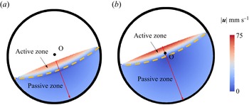
The steady velocity field for the granular flow in a rotating drum is illustrated in figure 17. The flat surfaces for both EV and EN symbolize the typical rolling mode. This is consistent with the Froude number ( $Fr=\omega ^2R/g$) criterion, i.e. the rolling mode occurs when
 $10^{-4}< Fr<10^{-2}$ (
 $Fr=9.79\times 10^{-4}$ in this case). Under this mode, the whole granular bed can be divided into two regions by a rigid body limit, such as the orange dashed curves in figure 17. In the literature, the area above the rigid body limit is termed the active zone, and the remaining area is termed the passive zone. In the passive zone, the granular material moves as a rigid body together with the drum. On the contrary, the grains in the active zone flow significantly faster than those from the underlying zone, and experience dramatic shearing.
Velocity field for the granular flow in a rotating drum at  $t=20$ s in cases (a) EV and (b) EN.

In this case, both segregation velocity ( $V$) and diffusivity (
 $D$) are varied and proportional to the shear rate (
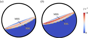
 $\dot \gamma$). Therefore, it is of considerable importance to analyse the global distribution of the shear rate, which is shown in figure 18. Here, rigid body limits similar to those in figure 17 are identified. We can find that in the passive zone, both EV and EN cases present almost zero shear rates, revealing the rigid motion of granular material as mentioned above. With a further step, the active zone is divided into two layers, respectively named as the upper active zone and the lower active zone in this study, separated by the maximum shearing surface, as shown by the white dotted line in figure 18. The shear rate in the upper active zone increases along the direction of gravity, while it decreases in the lower active zone. This division is useful for the segregation analysis, which will be given in the next subsection. For a better understanding, the shear rate distribution against the normalized mid-chord depth
 $\bar {d}_{mc}$ (cf. figure 17 for location) is drawn in figure 19. In both cases, the four curves are close to each other, indicating the steady-state flow condition.
Shear rate for the granular flow in a rotating drum at  $t=20$ s in cases (a) EV and (b) EN. Here, RBL and MSS are short for rigid body limit and maximum shearing surface, respectively.

Shear rate along the mid-chord for the cases (a) EV and (b) EN, at four time instances.

Comprehensive analysis of the granular flow has been conducted in our previous work (Zhu et al. Reference Zhu, Peng and Wu2022a), where both the inside and surface velocity fields of the grain assembly are presented. In this study, we focus on the discrepancy between the single-phase model adopted here and dual-constituent granular assembly in the real world. To achieve this, the velocity magnitude distributions along the mid-chord of the granular bed for both EV and EN cases are given in figures 20 and 21, aiming to demonstrate the capability of the proposed SPH model to reproduce properly the kinematic information of the granular flow in the rotating drum. A noticeable discrepancy between the velocity profiles from this study and Yang et al. (Reference Yang, Zheng, Bai and Yu2021) is observed in figures 20 and 21. In general, the SPH scheme gives a greater prediction to the velocity near the free surface than the Eulerian FEM. In comparison, high consistency among the results from all three methods is observed in the passive zone. When taking the DEM data as benchmark, an error analysis shows that SPH and the Eulerian FEM give similar accuracy. For instance, at  $t=40$ s, the MAE is equal to 0.42 and 0.43 cm s
 $^{-1}$ for the Eulerian FEM and SPH results, respectively, in the case of EV, but 0.29 and 0.17 cm s
 $^{-1}$ in the case of EN. The deviation in the numerical reproduction probably originates from the different numerical schemes adopted by the two studies. In the work of Yang et al. (Reference Yang, Zheng, Bai and Yu2021), the granular flow is modelled with the Eulerian FEM, the drum is taken as a Lagrangian structure immersed in the Eulerian domain, and the concentration information is updated with the finite difference method. In comparison, only one numerical method, i.e. SPH, is used in the current work for all aspects. Also, Yang et al. (Reference Yang, Zheng, Bai and Yu2021) adopts the immersed boundary method and the volume of fraction technique to realize the frictional contact boundary condition, which could lead to mass loss in simulation. In this study, the drum wall is simply assumed to be non-slip, and the Lagrangian nature of the SPH method ensures the mass conservation throughout the whole simulation. With regard to the computational cost, SPH usually can achieve a calculation efficiency with two orders using a consumer-level GPU card ascribed to its parallelism when compared to the similar numerical code run on a CPU card (Zhan et al. Reference Zhan, Peng, Zhang and Wu2019). The authors’ previous work shows that the calculation efficiency is improved approximately 100 times when comparing the time consumption of the SPH model from this study and that of the Eulerian FEM. More details can be found in Zhu et al. (Reference Zhu, Peng and Wu2022a) for readers with an interest in computation efficiency.
Velocity profile along the mid-chord of the granular bed in the case of EV at (a)  $t=20$ s, (b)
 $t=30$ s and (c)
 $t=40$ s. The scattered points are from the DEM simulation, while the dashed line represents the Eulerian FEM prediction from Yang et al. (Reference Yang, Zheng, Bai and Yu2021).

Velocity profile along the mid-chord of the granular bed in the case of EN at (a)  $t=20$ s, (b)
 $t=30$ s and (c)
 $t=40$ s. The scattered points are from the DEM simulation, while the dashed line represents the Eulerian FEM prediction from Yang et al. (Reference Yang, Zheng, Bai and Yu2021).

The previous study (Zhu et al. Reference Zhu, Peng and Wu2022a) reveals that the bed profile will remain stable after a half circulation in the rolling regime, indicating the formation of a steady-state velocity field. This explains the consistent velocity distribution along the mid-chord for all three time instants from both the SPH and Eulerian FEM predictions in figures 20 and 21, as the rotation rate in this case is fixed at 5 rpm. In comparison, an increment is observed in terms of the surface velocity obtained from the DEM simulation. For instance, in the case of EV, the surface velocity ascends from around 6 cm s $^{-1}$ at
 $t=20$ s to 7 cm s
 $^{-1}$ at
 $t=40$ s. The reason for this change could be twofold. One reason is that the flow layer will dilate due to the strong shearing. On the other hand, some grains on the free surface will collide and bounce into the air due to the inadequate resistance from the underlying granular bed, showing some gas properties. Therefore, an advanced constitutive model dictating the shear dilatancy and gas-like behaviour of the granular material is needed for a more precise prediction, but this is out of the scope of this study. In addition, the numerical result from the DEM simulation shows an almost identical velocity distribution between the small and large grains, which means that the segregation-induced percolation is negligible compared to the mean velocity. Therefore, the single-phase model adopted in this study can capture the kinematic information accurately. In general, both qualitative and quantitative satisfactions are achieved by the SPH model.
6.2. Segregation evolution
The correct implementation of the HCSR scheme is the prerequisite for predicting precisely the segregation evolution. Likewise, in this subsection, we first demonstrate the capability of the proposed HCSR scheme on boundary particle searching and normal direction identification in case of the rotating drum, which is shown in figures 22 and 23. Here, the geometry of the granular bed is more complex than that in the shear cell problem as the kinematic information is updated according to the momentum equation. Notwithstanding, the HCSR scheme still performs well with both EN and EV cases.
Boundary particle searching and classification in a rotating drum for cases (a) EN and (b) EV.

Normal direction of the boundary particles in a rotating drum for cases (a) EN and (b) EV.

Figures 24 and 25 present snapshots of the grain-size distribution for EV and EN cases from both DEM and SPH simulations, and are in good agreement with one another. In this case, particle segregation happens mainly in the active zone, where grains are subjected to severe shearing. When flowing through the active zone, the small grains migrate downwards and enrich the lower active zone, while the large grains float to the free surface and concentrate there. After entering into the passive zone, the granular materials rotate clockwise like a rigid body to the other side of the rigid body limit, and restart the segregation process in the active zone again. Such circulation repeats until reaching the dynamic equilibrium between the segregation and diffusion effects. The predictions for the concentration along the mid-chord from DEM and SPH are given in figure 26, from which we can find qualitative agreement between the results from these two methods. The discrepancy could originate from the following three aspects. First, as pointed out in Yang et al. (Reference Yang, Zheng, Bai and Yu2021), the concentration profile obtained from the DEM simulation will be influenced by the sample size (i.e. the specific area to calculate the average concentration) to a great degree. Second, the constitutive model that dictates the mechanical behaviour of granular materials plays a key role in kinematics, which will influence the segregation evolution through the shear rate. In this study, the simple  $\mu (I)$ elastoplasticity is employed to model the size-bidisperse granular assembly. This model could reproduce the major features, but some key aspects are missing, such as the shear dilatancy and the gas-like behaviour of the granular materials on the free surface. Therefore, a more advanced constitutive model is necessary for a better simulation result. Last, but not least, the parameters
 $V$ and
 $D$ are two key players in particle-size segregation, but have complex scaling laws with multiple factors (Trewhela et al. Reference Trewhela, Ancey and Gray2021a). In this study, (2.7a,b) is indeed simplified, and the coefficients
 $\chi _{D}$ and
 $\chi _{V}$ are calibrated from the oscillatory shear cell test.
Snapshots of grain distribution from the DEM (upper images, reprinted from Yang et al. Reference Yang, Zheng, Bai and Yu2021) and SPH (lower images) for the EV case. In the DEM, red and green particles denote large and small grains, respectively, while  $C$ represents the concentration of small grains in SPH.

Snapshots of grain distribution from the DEM (upper images, reprinted from Yang et al. Reference Yang, Zheng, Bai and Yu2021) and SPH (lower images) for the EN case. In the DEM, red and green particles denote large and small grains, respectively, while  $C$ represents the concentration of small grains in SPH.

Concentration along the mid-chord in the cases (a) EV and (b) EN. The scattered points represent the result from the DEM, and the solid lines denote the SPH prediction.

Figure 27 presents the temporal evolution of the system-wide concentration for small grains. In the cases EV and EN, the initial concentration is 0.5 and 0.11, respectively. These two values should stay constant due to the incompressibility assumption adopted in this study, as the scatters demonstrate in figure 27. Good consistency is found between the results from the SPH simulation and theory in both cases. In comparison, a slight divergence is observed in the EV case. The accuracy of the proposed HCSR scheme depends on the source term  $q$. According to (4.16), the key issue is to obtain the accurate normal vectors calculated with (4.10). In this process, some error will take place, and the discrepancy will be magnified by the value of the inhomogeneous Neumann boundary condition
 $f( C)$. As seen in figure 23, the majority of the calculated normal vectors are accurately perpendicular to the boundary, while on the free surface, the disorder can be found locally. This is believed to be the origin of the difference between the simulation and theory results. On the other hand, the concentration
 $C$ on the free surface is much smaller in the case of EN than EV (see figure 26), leading to the inhomogeneous Neumann boundary condition
 $f(C)$, of less significance for the former than the latter. This explains the better agreement in the EN case, as shown in figure 27. Therefore, higher accuracy is achievable with an improved algorithm for calculating the normal directions of those boundary particles, which deserves further study in the future. Nevertheless, satisfactory performance on concentration conservation is observed in the current proposed method.
Temporal evolution of global concentration for small grains.

In the following, we analyse the segregation mechanism behind the concentration evolution. From (2.10), we can find that a dynamic equilibrium will be reached finally under the effect of segregation and diffusion. In particular, two factors promote the particle segregation: the vertical gradients of concentration  $\boldsymbol {\nabla }_{g}C$, and the segregation velocity
 $\boldsymbol {\nabla }_{g}V$. The latter takes no effect when the segregation velocity is assumed constant, such as in the benchmark problem in § 5.1. In comparison,
 $\boldsymbol {\nabla }_{g}V$ rather than
 $\boldsymbol {\nabla }_{g}C$ triggers the segregation in the rotating drum as the concentration is globally homogeneous at the initial stage. Figures 28 and 29 illustrate the spatial distribution of the concentration rate along the mid-chord and its three components caused by
 $-F\,\boldsymbol {\nabla }_{g}V$,
 $-V\mathcal {F}\,\boldsymbol {\nabla }_{g}C$ and
 $\boldsymbol {\nabla }(D\,\boldsymbol {\nabla } C )$, denoted as
 $\dot C_1$,
 $\dot C_2$ and
 $\dot C_3$.
Concentration rate distribution along the mid-chord for the EN case at (a)  $t=5$ s, (b)
 $t=10$ s, (c)
 $t=20$ s and (d)
 $t=40$ s, with
 $\dot C_{1}$,
 $\dot C_{2}$ and
 $\dot C_{3}$ representing the contributions from
 $-F\,\boldsymbol {\nabla }_{g}V$,
 $-V\mathcal {F}\,\boldsymbol {\nabla }_{g}C$ and
 $\boldsymbol {\nabla }(D\,\boldsymbol {\nabla } C )$.

Concentration rate distribution along the mid-chord for the EV case at (a)  $t=5$ s, (b)
 $t=10$ s, (c)
 $t=20$ s and (d)
 $t=40$ s, with
 $\dot C_{1}$,
 $\dot C_{2}$ and
 $\dot C_{3}$ representing the contributions from
 $-F\,\boldsymbol {\nabla }_{g}V$,
 $-V\mathcal {F}\,\boldsymbol {\nabla }_{g}C$ and
 $\boldsymbol {\nabla }(D\,\boldsymbol {\nabla } C )$.

(1) Effect of vertical gradient of segregation velocity,  $-F\boldsymbol {\nabla }_{g}V$. It is observed that
 $\dot C_1$ plays the dominant role in the concentration evolution, particularly at the beginning such as at
 $t=5$ s. In figure 28,
 $\dot C_1$ ascends monotonically from a negative point on the free surface to the peak value as
 $\bar {d}_{mc}$ increases, and then plummets to zero at approximately
 $\bar {d}_{mc}=0.24$, after which
 $\dot C_1=0$ holds until the drum wall. Also, both the starting point and the peak value rise as the segregation proceeds. The reason for the change is twofold. On the one hand, the velocity field after
 $t=5$ s reaches the steady state, and the radial shear rate
 $\dot \gamma$ appears quadratic (figure 19), leading to the constant distribution of
 $\boldsymbol {\nabla }_{g}V$ along the mid-chord. On the other hand, as the segregation develops, the concentration
 $C$ decreases in the upper active zone and increases in lower part, leading to the smaller segregation function
 $F$ in the upper active zone and greater
 $F$ in the lower active zone. A similar change is found in the EV case, but
 ${\dot C}_1$ decreases in both zones. This difference originates from the fact that the initial concentration is 0.5 in the EV case, while it is 0.11 in the EN case. As a result, the segregation function
 $F$ in the EV case drops in the whole active zone as the segregation develops.
(2) Effect of vertical gradient of concentration,  $-V\mathcal {F}\boldsymbol {\nabla }_{g}C$. The effect of
 ${\dot C}_2$ is initially insignificant compared to
 ${\dot C}_1$, but its contribution becomes more pronounced as segregation develops, due to the increasing vertical concentration gradient
 $\boldsymbol {\nabla }_{g}C$ in the active zone. As time proceeds,
 ${\dot C}_2$ approaches a quadratic distribution as
 $\dot \gamma$ does, indicating the dominant influence of shear rate in
 ${\dot C}_2$. Here,
 $\mathcal {F}$ is another key factor determining the magnitude of
 ${\dot C}_2$. Due to the application of the symmetric form of the segregation function here,
 $\mathcal {F}=0$ holds when
 $C=0.5$. As a result,
 ${\dot C}_2$ shrinks to zero near
 $\bar d_{mc}=0.1$ in the EV case, as shown in figure 29. Furthermore, the sign of
 ${\dot C}_2$ is determined by
 $\mathcal {F}$ since both
 $V$ and
 $\boldsymbol {\nabla }_{g}C$ are positive in most parts of the active zone.
(3) Effect of diffusion,  $\boldsymbol {\nabla }(D\,\boldsymbol {\nabla } C )$. First, an apparent drop in
 ${\dot C}_3$ is observed on the free surface as time proceeds. This is ascribed to the fact that the source term
 $q$ in (4.7) will become insignificant when
 $C$ gets close to zero or unity. A minor role is played by
 ${\dot C}_3$ in the remaining active zone during the whole process. This is because the effect of
 ${\dot C}_3$ in figures 28 and 29 could be understood approximately as the description of the curvature of the concentration distribution along the mid-chord. From figure 26, it is found that in the active domain, the concentration distribution is quite close to being linear. Therefore, the diffusion effect, in general, is insubstantial. Note that in this simulation, only 40 seconds are reproduced and the steady state has not been reached yet. Otherwise, the magnitude of the segregation and diffusion should be equal but opposite.
7. Conclusions
This work proposes a continuum-based numerical method within the SPH framework, providing a novel approach to studying particle segregation in a bidisperse-sized granular system. The particle assembly is taken as single phase with varying concentration for each constituent, and the segregation evolution is governed by the segregation–diffusion equation. The developed SPH model is first examined with a benchmark problem, a shear box, and performs well, with excellent agreement with the experimental result. Then a detailed numerical investigation is conducted to explore the particle segregation mechanism in the granular flow in a rotating drum, with some key conclusions as follows.
(i) The spatially varying shear rate, which determines the segregation velocity and diffusivity, triggers the particle segregation in the rotating drum from the continuum perspective.
(ii) The particle segregation takes place mainly in the active zone, where granular material experiences severe shearing, while the grains in the passive zone move together with the drum as a rigid body.
(iii) The vertical gradient of segregation velocity plays the dominant role in the particle segregation, particularly at the beginning of the whole process.
Funding
The authors wish to acknowledge the financial support from OeAD WTZ project (grant no. CN14/2021). The first author wishes to thank the Otto Pregl Foundation for financial support in Austria.
Declaration of interests
The authors report no conflict of interest.
Appendix A
In this appendix, we explain why the indirect SPH formulation (2.10) outperforms the original version (2.5) in terms of accuracy. As mentioned in the main text, the segregation flux could have complex spatial distribution. For simplicity, assume that the segregation velocity  $V(C(\boldsymbol x))$ is constantly equal to 1, so the segregation flux could be reduced as
 $Q(\boldsymbol x)=F(C(\boldsymbol x))$. Without loss of generality, the asymmetric flux model is adopted with
 $A=1.33$ and
 $\kappa =0.89$. As we proceed, the concentration distribution is assumed to be quadratic in coordinate
 $z$ such that
 \begin{equation} C(z)=4z(1-z). \end{equation}
As a result, with the explicit expressions of the segregation flux,  $\boldsymbol {\nabla }_{g}Q$ is derivable analytically. On the other hand,
 $\boldsymbol {\nabla }_{g}Q$ could also be obtained with the SPH method. The final results for
 $\boldsymbol {\nabla }_{g}Q$ from the analytical solution and the two SPH approximation schemes are drawn in figure 30, where the root mean square errors between the numerical and analytical methods are also provided. From the figure, a better agreement between the numerical and analytical solutions is observed for the indirect scheme than the direct one, indicating the superiority of the indirect SPH approximation scheme over the direct one regarding calculation accuracy, which is also revealed intuitively by the RMSE data.
Numerical predictions for  $\boldsymbol {\nabla }_{g}Q$ with concentration in the quadratic distribution: (a) indirect SPH approximation; (b) direct SPH approximation.

Notice that the analysis above is made upon two simplifications, i.e. (i) the segregation velocity is assumed constant, and (ii) the concentration distribution is no more complex than the cubic function. Considering this, it is foreseeable that the error induced by the direct SPH approximation to  $\boldsymbol {\nabla }_{g}Q$ in a realistic segregation simulation would be more pronounced than the mathematical example shown here.
Appendix B
In this appendix, a brief introduction to deriving (2.16) within the elasto-perfectly plastic theoretical framework is presented. For a granular material that is located at the yield surface, the following equation holds:
 \begin{equation} f( \sigma_{ij})=0. \end{equation}
Therefore one can get
 \begin{equation} \dot{f}=\dfrac{\partial f}{\partial \sigma_{ij}}\,\dot\sigma_{ij}=0. \end{equation}
Within the plasticity theory, the relation between the stress increment and the elastic strain is dictated by Hooke's law as
 \begin{equation} \dot\sigma_{ij}=D_{ijkl}\varepsilon^{e}_{kl}=D_{ijkl}( \dot\varepsilon_{kl}-\dot\varepsilon^{p}_{kl}). \end{equation}
In this equation, the superscripts  $e$ and
 $p$ denote the elastic and plastic parts. The plasticity theory usually assumes that the plastic strain rate (or increment) can be determined by the so-called flow rule, reading
 \begin{equation} \dot\varepsilon^{p}_{ij}=\dot\lambda\,\dfrac{\partial g}{\partial \sigma_{ij}}. \end{equation}
Substituting (B3) and (B4) into (B2) yields the generic expression for the plastic multiplier  $\dot \lambda$ such that
 \begin{equation} \dot\lambda=\dfrac{\dfrac{\partial f}{\partial \sigma_{ij}}\,D_{ijkl}\dot\varepsilon_{kl}}{\dfrac{\partial f}{\partial \sigma_{ij}}\,D_{ijkl}\,\dfrac{\partial g}{\partial \sigma_{ij}}}. \end{equation}
To this end, (2.16) is derivable once the expressions for the yield and plastic potential functions, i.e. (2.11) and (2.15), are substituted into (B3) and (B5).
Note that the brief introduction to the plasticity theory provided here is mainly for the readership from the fluid community. More details are available from plasticity theory books (e.g. Yu Reference Yu2007).
Appendix C
The one-step return mapping scheme as introduced in § 2.4 starts with the elastic prediction at the beginning of a specific time step  $n$, as follows:
 \begin{equation} \Delta{\boldsymbol \sigma} = ( \dot{\boldsymbol \omega}\boldsymbol\sigma - \boldsymbol \sigma\dot{\boldsymbol \omega} + 2G\dot{\boldsymbol e} + K \dot\varepsilon_v\boldsymbol{\mathsf{I}})\,\Delta t, \end{equation}
where  $\Delta t$ is the time step, which is given in § 3.3. Afterwards, the yield criterion will be checked. When the predicted stress
 ${\boldsymbol \sigma }^*={\boldsymbol \sigma }^n+\Delta {\boldsymbol \sigma }$ is located within the yield surface, i.e.
 $f({\boldsymbol \sigma }^*)\leq 0$, the whole loading process is elastic, and the new stress can be updated directly with
 ${\boldsymbol \sigma }^{n+1}={\boldsymbol \sigma }^*$. Otherwise, a correction procedure will be activated to pull the stress point back to the yield surface, as the flowchart in figure 31 shows (where the variables with superscript
 $*$ are related to the predicted stress state). With the updated stress state as the input data for the next time step, the calculation loop can proceed until the end of the simulation.
Flow chart of the one-step return-mapping algorithm for the elasto-perfectly plastic model with Drucker–Prager yield criterion.

Appendix D
In this appendix, the mathematical deduction for the kernel approximation of the diffusion term, i.e. (3.5), will be presented.
Based on Taylor's theorem, the right-hand side of (3.5) can be rewritten as
 \begin{equation} \int_{\varOmega}[2g(\boldsymbol x)-\boldsymbol{\nabla} g(\boldsymbol x)\boldsymbol{\cdot}\Delta \boldsymbol x^\prime]\left[\boldsymbol{\nabla} f(\boldsymbol x)\boldsymbol{\cdot}\Delta \boldsymbol x^\prime-\dfrac{1}{2}\,{\Delta \boldsymbol x}^{\prime\textrm{T}}\,H_f(\boldsymbol x)\,{\Delta \boldsymbol x^\prime}\right]\dfrac{{\Delta \boldsymbol x^\prime}}{\| {\Delta \boldsymbol x^\prime}\| ^2}\boldsymbol{\cdot}\boldsymbol{\nabla}_{\boldsymbol{x}}W({\Delta \boldsymbol x^\prime},h)\,{\rm d}\kern0.06em \boldsymbol x^\prime, \end{equation}
where  $\Delta \boldsymbol x^\prime ={\boldsymbol x}-{\boldsymbol x^\prime }$, and
 $H_f(\boldsymbol x)$ denotes the Hessian of
 $f$ evaluated at
 $\boldsymbol x$ with the following specific form:
 \begin{equation} H_f(\boldsymbol x)=\begin{bmatrix} \dfrac{\partial^2f}{\partial x^2} & \dfrac{\partial^2f}{\partial x\,\partial y} & \dfrac{\partial^2f}{\partial x\,\partial z}\\ \dfrac{\partial^2f}{\partial y\,\partial x} & \dfrac{\partial^2f}{\partial y^2} & \dfrac{\partial^2f}{\partial y\,\partial z}\\ \dfrac{\partial^2f}{\partial z\,\partial x} & \dfrac{\partial^2f}{\partial z\,\partial y} & \dfrac{\partial^2f}{\partial z^2} \end{bmatrix}. \end{equation}
There are 144 terms in (D1) for a three-dimensional problem if we expand it as polynomials. This seems of high complexity, but can be simplified greatly if we take advantage of the odd and even properties.
First, we notice that  $g(\boldsymbol x)$,
 ${\Delta \boldsymbol x}^{\prime \textrm {T}}\,H_f(\boldsymbol x)\,{\Delta \boldsymbol x^\prime }$ and
 ${\Delta \boldsymbol x^\prime }\boldsymbol {\cdot }\boldsymbol {\nabla }_{\boldsymbol {x}}W({\Delta \boldsymbol x^\prime },h)$ are even functions of
 $\Delta \boldsymbol x^\prime$, while both
 $\boldsymbol {\nabla } g(\boldsymbol x)\boldsymbol {\cdot } \Delta \boldsymbol x^\prime$ and
 $\boldsymbol {\nabla } f(\boldsymbol x)\boldsymbol {\cdot } \Delta \boldsymbol x^\prime$ are odd. Consequently, the following identities hold:
 $$\begin{gather} \int_{\varOmega}[2g(\boldsymbol x)\,\boldsymbol{\nabla} f(\boldsymbol x)\boldsymbol{\cdot}\Delta \boldsymbol x^\prime]\,\dfrac{{\Delta \boldsymbol x^\prime}}{\| {\Delta \boldsymbol x}\| ^2}\boldsymbol{\cdot}\boldsymbol{\nabla}_{\boldsymbol{x}}W({\Delta \boldsymbol x^\prime},h)\,{\rm d}\kern0.06em \boldsymbol x^\prime =0, \end{gather}$$
 $$\begin{gather}\int_{\varOmega}[\boldsymbol{\nabla} g(\boldsymbol x)\boldsymbol{\cdot}\Delta \boldsymbol x^\prime\,{\Delta \boldsymbol x}^{\prime\textrm{T}}\,H_f(\boldsymbol x)\,{\Delta \boldsymbol x^\prime}]\,\dfrac{{\Delta \boldsymbol x^\prime}}{2\| {\Delta \boldsymbol x^\prime}\| ^2}\boldsymbol{\cdot}\boldsymbol{\nabla}_{\boldsymbol{x}}W({\Delta \boldsymbol x^\prime},h)\,{\rm d}\kern0.06em \boldsymbol x^\prime=0. \end{gather}$$
Therefore, (D1) can be reduced as
 \begin{equation} -\int_{\varOmega}[g(\boldsymbol x)\,{\Delta \boldsymbol x}^{\prime\textrm{T}}\,H_f(\boldsymbol x)\,{\Delta \boldsymbol x^\prime}+\boldsymbol{\nabla} g(\boldsymbol x)\boldsymbol{\cdot}\Delta \boldsymbol x^\prime\,\boldsymbol{\nabla} f(\boldsymbol x)\boldsymbol{\cdot}\Delta \boldsymbol x^\prime]\,\dfrac{{\Delta \boldsymbol x^\prime}}{\| {\Delta \boldsymbol x^\prime}\|^2}\boldsymbol{\cdot}\boldsymbol{\nabla}_{\boldsymbol{x}}W({\Delta \boldsymbol x^\prime},h)\,{\rm d}\kern0.06em \boldsymbol x^\prime. \end{equation}
For the sake of clarity, (D5) is rewritten in index notation:
 \begin{equation} -\iiint \left[g( x_l)\,\dfrac{\partial^2f}{\partial x_i\,\partial x_j}\,\Delta x_i^\prime\,\Delta x_j^\prime+\dfrac{\partial g}{\partial x_i}\,\dfrac{\partial f}{\partial x_j}\,\Delta x_i^\prime\,\Delta x_j^\prime\right]\dfrac{\Delta x_k^\prime}{\Delta x_m^\prime\,\Delta x_m^\prime}\,\dfrac{\partial W}{\partial x_k^\prime} \,{\rm d}\kern0.06em x_1^\prime \,{\rm d}\kern0.06em x_2^\prime \,{\rm d}\kern0.06em x_3^\prime, \end{equation}
where  $x$ with roman subscripts (
 $=1, 2, 3$) denotes the Cartesian coordinates, and the Einstein summation convention is adopted. In the following, we will prove that
 \begin{equation} \iiint\dfrac{\Delta x_i^\prime\,\Delta x_j^\prime\,\Delta x_k^\prime}{\Delta x_m^\prime\,\Delta x_m^\prime}\,\dfrac{\partial W}{\partial x_k^\prime} \,{\rm d}\kern0.06em x_1^\prime \,{\rm d}\kern0.06em x_2^\prime \,{\rm d}\kern0.06em x_3^\prime=\begin{cases} 0, & i\neq j,\\ -1, & i=j. \end{cases} \end{equation}
There are two cases when  $i\neq j$, i.e.
 $i\neq j\neq k$ and
 $k=i\neq j$ (or
 $k=j\neq i$). The integrand in (D7) is asymmetric over
 $\Delta x_i^\prime$ and
 $\Delta x_j^\prime$ in the former condition, and an odd function about
 $\Delta x_k^\prime$ and
 $\Delta x_j^\prime$ (or
 $\Delta x_i^\prime$) in the latter, so its integral is null. The next step is to validate that the left-hand side of (D7) is equal to minus unity when
 $i=j$. For this purpose, the left-hand side of (D7) is first rewritten in spherical coordinates:
 \begin{equation} \iiint\Delta x_i^{\prime 2}\,\dfrac{\partial W}{\partial\rho}\,\rho \sin\varphi \,{\rm d}\rho \,{\rm d}\theta \,{\rm d}\varphi. \end{equation}
Here, the origin of the spherical coordinate system is located at point  $\boldsymbol x$, and the conversion formulas between the Cartesian and spherical coordinates are
 \begin{equation} \left.\begin{aligned} \Delta x_1^\prime &=\rho\sin\varphi\cos\theta,\\ \Delta x_2^\prime &=\rho\sin\varphi\sin\theta,\\ \Delta x_3^\prime &=\rho\cos\varphi, \end{aligned}\right\} \end{equation}
with the following restrictions on the coordinates:
 \begin{equation} \left.\begin{aligned} \rho &\in[0,2h],\\ \theta&\in[0,2{\rm \pi}],\\ \varphi&\in[0,{\rm \pi}]. \end{aligned}\right\} \end{equation}
Substituting (D9) into (D8) yields the same equation for  $i=1,2,3$, as follows:
 \begin{equation} \int_{0}^{2h}\dfrac{4}{3}\,{\rm \pi}\rho^3\,\dfrac{\partial W}{\partial \rho}\,{\rm d}\rho. \end{equation}
Notice that due to the compact support condition of the kernel function, we have
 \begin{equation} \int_{0}^{2h}{\rm d}\left( \dfrac{4}{3}\,{\rm \pi}\rho^3W\right) =\int_{0}^{2h}\dfrac{4}{3}\,{\rm \pi}\rho^3\,\dfrac{\partial W}{\partial \rho}\, {\rm d}\rho+\int_{0}^{2h}W\,{\rm d}\left( \dfrac{4}{3}\,{\rm \pi}\rho^3\right)=0. \end{equation}
The second term in the middle of this equation is indeed the unity condition of the kernel function, indicating that its value is 1. Finally, it is verified that (D11) is equal to minus unity.
Substituting (D7) into (D6) yields
 \begin{equation} g\,\dfrac{\partial^2f}{\partial x_i\,\partial x_i}+\dfrac{\partial g}{\partial x_i}\,\dfrac{\partial f}{\partial x_i}. \end{equation}
This expression is exactly the index notation form of the left-hand side of (3.5).
Appendix E
This appendix presents the derivation of SPH approximation for  $\boldsymbol {\nabla }_{g}C$ and
 $\boldsymbol {\nabla }_{g}V$ with
 $C^1$ consistency. In the following, the symbol
 $X$ will be used to represent
 $C$ and
 $V$. The process starts with the Taylor series as follows:
 \begin{equation} X(\boldsymbol x^\prime)=X(\boldsymbol x) -\boldsymbol{\nabla} X(\boldsymbol x)\boldsymbol{\cdot}\Delta\boldsymbol x^\prime+O(h^2). \end{equation}
Multiplying by  $W(\Delta \boldsymbol x^\prime,h)$ or
 $\boldsymbol {\nabla } W_{\boldsymbol x}(\Delta \boldsymbol x^\prime,h)$ on both sides of (E1), and integrating over domain
 $\varOmega$, gives
 \begin{equation} \begin{bmatrix} B_1\\ B_2 \end{bmatrix}=\begin{bmatrix} C_{11} & C_{12}\\ C_{21} & C_{22} \end{bmatrix} \begin{bmatrix} X(\boldsymbol x)\\ \boldsymbol{\nabla} X(\boldsymbol x) \end{bmatrix}, \end{equation}
with
 $$\begin{gather} B_1=\int_{\varOmega}X(\boldsymbol x^\prime)\,W(\Delta \boldsymbol x^\prime,h)\,{\rm d}\kern0.06em \boldsymbol x^\prime, \end{gather}$$
 $$\begin{gather}B_2=\int_{\varOmega}X(\boldsymbol x^\prime)\,\boldsymbol{\nabla} W_{\boldsymbol x}(\Delta \boldsymbol x^\prime,h)\,{\rm d}\kern0.06em \boldsymbol x^\prime, \end{gather}$$
 $$\begin{gather}C_{11}=\int_{\varOmega}W(\Delta \boldsymbol x^\prime,h) \,{\rm d}\kern0.06em \boldsymbol x^\prime, \end{gather}$$
 $$\begin{gather}C_{12}=-\int_{\varOmega}\Delta\boldsymbol x^\prime\,W(\Delta \boldsymbol x^\prime,h)\,{\rm d}\kern0.06em \boldsymbol x^\prime, \end{gather}$$
 $$\begin{gather}C_{21}=\int_{\varOmega}\boldsymbol{\nabla} W_{\boldsymbol x}(\Delta \boldsymbol x^\prime,h)\,{\rm d}\kern0.06em \boldsymbol x^\prime, \end{gather}$$
 $$\begin{gather}C_{22}=-\int_{\varOmega} \boldsymbol{\nabla} W_{\boldsymbol x}(\Delta \boldsymbol x^\prime,h)\otimes\Delta\boldsymbol x^\prime \,{\rm d}\kern0.06em \boldsymbol x^\prime. \end{gather}$$
Note that the remainder is neglected during the process. In (E2), only  $X(\boldsymbol x)$ and
 $\boldsymbol {\nabla } X(\boldsymbol x)$ are the unknowns, as the integrals are deterministic for an arbitrary point
 $\boldsymbol x$. Thus the number of unknowns is consistent with the order of the equation set, which is a solvable problem. The particle approximation of (E3)–(E8) is
 $$\begin{gather} B_1=\sum_{j\in\varOmega}X(\boldsymbol x_j)\,W_{ij}m_j/\rho_j, \end{gather}$$
 $$\begin{gather}B_2=\sum_{j\in\varOmega}X(\boldsymbol x_j)\,\boldsymbol{\nabla}_iW_{ij}m_j/\rho_j, \end{gather}$$
 $$\begin{gather}C_{11}=\sum_{j\in\varOmega}W_{ij}m_j/\rho_j, \end{gather}$$
 $$\begin{gather}C_{12}=-\sum_{j\in\varOmega}\boldsymbol x_{ij}W_{ij}m_j/\rho_j, \end{gather}$$
 $$\begin{gather}C_{21}=\sum_{j\in\varOmega}\boldsymbol{\nabla}_iW_{ij}m_j/\rho_j, \end{gather}$$
 $$\begin{gather}C_{22}=-\sum_{j\in\varOmega}\boldsymbol{\nabla}_iW_{ij}\otimes\boldsymbol x_{ij}m_j/\rho_j. \end{gather}$$
After obtaining the value of  $\boldsymbol {\nabla } X(\boldsymbol x)$,
 $\boldsymbol {\nabla }_{g}X(\boldsymbol x)$ can be determined through
 \begin{equation} \boldsymbol{\nabla}_{g}X(\boldsymbol x)=\dfrac{\boldsymbol g}{\|\boldsymbol g \| }\boldsymbol{\cdot}\boldsymbol{\nabla} X(\boldsymbol x). \end{equation}