1 Introduction
Droplet dynamics has been an progressively rising topic of interest due to its wide gamut of applications in various microfluidic devices (Stone, Stroock & Ajdari Reference Stone, Stroock and Ajdari2004; Baroud, Gallaire & Dangla Reference Baroud, Gallaire and Dangla2010; Seemann et al. Reference Seemann, Brinkmann, Pfohl and Herminghaus2012). Some of these applications are cell encapsulation, drug delivery, analytical detection and reagent mixing (Di Carlo et al. Reference Di Carlo, Irimia, Tompkins and Toner2007; Huebner et al. Reference Huebner, Sharma, Srisa-Art, Hollfelder, Edel and Demello2008; Teh et al. Reference Teh, Lin, Hung and Lee2008; Baroud et al. Reference Baroud, Gallaire and Dangla2010; Zhu & Fang Reference Zhu and Fang2013). The transport of droplets and bubbles also finds applications in the manufacture of pure materials (Kim et al. Reference Kim, Jeon, Choi, Shim, Kim and Yang2014; Sajeesh & Sen Reference Sajeesh and Sen2014; Anna Reference Anna2016; Murr & Johnson Reference Murr and Johnson2017). With the advent of space exploration, studies on droplet dynamics under microgravity environments are becoming more and more important (Subramanian Reference Subramanian1983; Balasubramaniam & Lavery Reference Balasubramaniam and Lavery1989; Pak, Feng & Stone Reference Pak, Feng and Stone2014; Das et al. Reference Das, Mandal, Som and Chakraborty2017). The motion of the droplets in this scenario is solely due to variation in interfacial tension or due to any imposed flow, if present. Moreover, the transverse migration of droplets as well as their steady-state position in a channel gives an idea of the distribution of droplets, which in turn is of great importance in determining the flow rate though the channel for a given pressure drop (Ward et al. Reference Ward, Faivre, Abkarian and Stone2005; Kinoshita et al. Reference Kinoshita, Kaneda, Fujii and Oshima2007; Anna Reference Anna2016).
It has been shown that an eccentrically placed droplet in a Poiseuille flow field undergoes migration only in the axial direction in the absence of droplet deformation, surfactants or fluid viscoelasticity (Hetsroni & Haber Reference Hetsroni and Haber1970; Chan & Leal Reference Chan and Leal1979). In the Stokes flow limit, various theoretical studies have shown that the presence of any of the abovementioned effects causes the cross-stream migration of droplets in a pressure driven flow (Chan & Leal Reference Chan and Leal1979; Nas & Tryggvason Reference Nas and Tryggvason2003; Stan et al.
Reference Stan, Guglielmini, Ellerbee, Caviezel, Stone and Whitesides2011; Wu & Hu Reference Wu and Hu2011; Pak et al.
Reference Pak, Feng and Stone2014; Mandal, Bandopadhyay & Chakraborty Reference Mandal, Bandopadhyay and Chakraborty2015; Bandopadhyay et al.
Reference Bandopadhyay, Mandal, Kishore and Chakraborty2016). Other than these, two-dimensional (2-D) numerical simulations using the boundary integral method have also been carried out to study the migration of deformable droplets in a pressure driven flow at zero Reynolds number (Zhou & Pozrikidis Reference Zhou and Pozrikidis1993, Reference Zhou and Pozrikidis1994). Mortazavi & Tryggvason (Reference Mortazavi and Tryggvason2000) studied numerically the cross-stream migration of a deformable droplet in a 2-D Poiseuille flow (Mortazavi & Tryggvason Reference Mortazavi and Tryggvason2000); they showed that under the low-Reynolds-number limit, for
 $\unicode[STIX]{x1D706}=0.125$
, the droplet always migrates towards the centreline of the channel, whereas for
 $\unicode[STIX]{x1D706}=1$
, the droplet moves away from the centreline of the channel. Here,
 $\unicode[STIX]{x1D706}$
is the ratio of viscosities of the droplet phase and the carrier phase.
The use of external effects like electric (Ahn et al.
Reference Ahn, Kerbage, Hunt, Westervelt, Link and Weitz2006; Link et al.
Reference Link, Grasland-Mongrain, Duri, Sarrazin, Cheng, Cristobal, Marquez and Weitz2006; Mandal, Bandopadhyay & Chakraborty Reference Mandal, Bandopadhyay and Chakraborty2016), acoustic (Seemann et al.
Reference Seemann, Brinkmann, Pfohl and Herminghaus2012), thermal (Young, Goldstein & Block Reference Young, Goldstein and Block1959; Balasubramaniam & Subramaniam Reference Balasubramaniam and Subramaniam1996; Karbalaei, Kumar & Cho Reference Karbalaei, Kumar and Cho2016) and magnetic (Seemann et al.
Reference Seemann, Brinkmann, Pfohl and Herminghaus2012) has been of great importance in recent times due to their wide application in a variety of fields. The presence of these external fields introduces a jump in stress at the droplet interface which alters the net hydrodynamic force acting on the droplet, and hence the droplet dynamics changes. In the present study, we have focused on the effect of temperature variation in the flow field. The variation of temperature along the droplet surface develops a Marangoni stress, which drives the droplet even in a quiescent medium. This is called thermocapillary migration and was first demonstrated experimentally and theoretically by Young et al. (Reference Young, Goldstein and Block1959). Following their study, the effects of several aspects like fluid inertia (Haj-Hariri, Nadim & Borhan Reference Haj-Hariri, Nadim and Borhan1990), droplet deformation (Nadim, Haj-Hariri & Borhan Reference Nadim, Haj-Hariri and Borhan1990), bounding wall (Meyyappan & Subramanian Reference Meyyappan and Subramanian1987; Barton & Shankar Subramanian Reference Barton and Shankar Subramanian1990; Barton & Subramanian Reference Barton and Subramanian1991; Chen Reference Chen1999, Reference Chen2003) and thermal convection (Zhang, Subramanian & Balasubramaniam Reference Zhang, Subramanian and Balasubramaniam2001; Balasubramaniam & Subramanian Reference Balasubramaniam and Subramanian2004; Yariv & Shusser Reference Yariv and Shusser2006) on the thermocapillary migration of a droplet suspended in a quiescent medium were studied. Wang et al. and Hariri et al. performed three-dimensional (3-D) numerical simulations to study the thermocapillary migration of deformable as well as non-deformable droplets for finite values of thermal Marangoni number
 $(Ma_{T})$
, which signifies the ratio of the thermally induced Marangoni stress to the viscous stresses acting on the droplet (Haj-Hariri, Shi & Borhan Reference Haj-Hariri, Shi and Borhan1997; Wang et al.
Reference Wang, Lu, Wang, Yang and Mao2008). Balasubramaniam & Subramaniam (Reference Balasubramaniam and Subramaniam1996) found that for large values of
 $Ma_{T}$
, the droplet velocity increases with increase of
 $Ma_{T}$
. In recent work, Raja Shekhar and co-workers have theoretically shown the combined effect of imposed Poiseuille flow as well as the thermal Marangoni stress on the droplet dynamics (Choudhuri & Raja Sekhar Reference Choudhuri and Raja Sekhar2013). In their work, they showed that in the absence of surfactants, fluid inertia and droplet deformation, a linear combination of the migration velocity due to the thermocapillary effect and that due to the imposed flow gives us the final droplet migration velocity. Studies performed by Baroud et al. (Reference Baroud, Gallaire and Dangla2010) clearly indicate the use of thermocapillarity as a tool to control droplet transverse position in a microfluidic channel. Robert de Saint Vincent, Wunenburger & Delville (Reference Robert de Saint Vincent, Wunenburger and Delville2008) used a laser beam to sort droplets possessing different thermal diffusivities from one another. These results exemplify the fact that thermally modulated manipulation of droplets has diverse applications in the field of microfluidics and motivates us strongly to take up the initiative to discover new perspectives that govern the essential physics of interest. The mathematical model used in the present study, from that perspective, takes into account the deformation of the droplet in a non-isothermal Poiseuille flow field, which has not been previously considered. However, various simplified versions of this model have been considered by a number of researchers (Kim & Subramanian Reference Kim and Subramanian1989; Pak et al.
Reference Pak, Feng and Stone2014) in the past.
Considerable research endeavour has been made to demonstrate the effect of temperature variation as well as imposed flow on droplet migration characteristics, both theoretically and numerically. A number of studies have been focused towards active control over motion as well as shape deformation of droplets in microchannels (Teh et al. Reference Teh, Lin, Hung and Lee2008; Casadevall i Solvas & DeMello Reference Casadevall i Solvas and DeMello2011; Stan et al. Reference Stan, Guglielmini, Ellerbee, Caviezel, Stone and Whitesides2011; Seemann et al. Reference Seemann, Brinkmann, Pfohl and Herminghaus2012; Anna Reference Anna2016) for lab-on-chip applications as well as drug delivery, cell encapsulation and analytic detection. However, in the literature, there is no reported study that deals with the temperature-induced cross-stream migration of a deformable droplet in a Poiseuille flow, either by using asymptotic theory for the case of an unbounded flow or by employing numerical simulations in the presence of a fluidic confinement. In the present study, accordingly, we focus on the simultaneous effect of a transverse temperature gradient as well as shape deformation on the dynamic evolution of the droplet under such incipient flow conditions. One unique aspect that hallmarks the non-triviality of the problem at hand is the fact the net effect cannot be trivially perceived as a linear superposition of the influences of the flow components due to the thermocapillary driven Marangoni stress and the Poiseuille flow as a consequence of the intrinsic nonlinearities associated with the shape deformation of the droplet. As a result, our analytical and numerical studies yield non-intuitive characteristics of the droplet evolution under this combined field, which may turn out to have profound consequences for the fine tuning of a desired transverse distribution of droplets in a micro-confined flow.
2 Problem formulation
2.1 Physical system
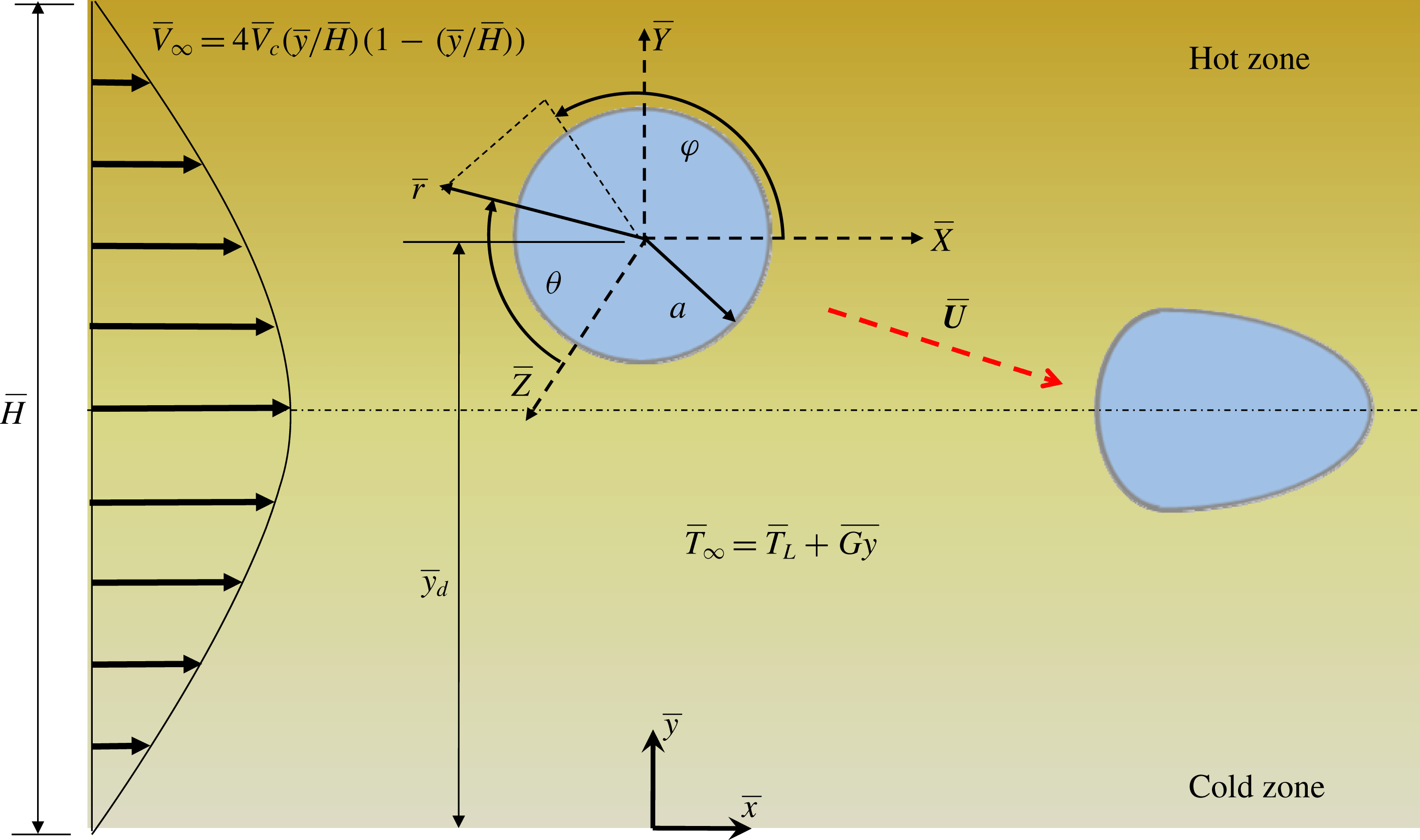
The present problem deals with a viscous Newtonian droplet of radius
 $a$
, having density
 $\unicode[STIX]{x1D70C}_{i}$
, thermal conductivity
 $k_{i}$
and viscosity
 $\unicode[STIX]{x1D707}_{i}$
. This droplet is suspended in another Newtonian fluid of thermal conductivity
 $k_{e}$
, density
 $\unicode[STIX]{x1D70C}_{e}$
and viscosity
 $\unicode[STIX]{x1D707}_{e}$
in a parallel plate microchannel. The subscripts ‘
 $e$
’ and ‘
 $i$
’ signify the carrier phase and droplet phase properties or quantities respectively. The droplet is placed in an off-centre position, above the centreline of the microchannel, as can be seen from the schematic in figure 1. A rectangular Cartesian coordinate system
 $(\bar{x},\bar{y})$
is adopted, which is attached to the bottom plate (figure 1). For the purpose of analytical treatment, the droplet is assumed to be much smaller than the width of the channel. Hence, the suspending medium in the schematic in figure 1 is effectively shown to be unbounded. In figure 1,
 $\bar{y}_{d}$
represents the transverse position of the droplet measured from the
 $\bar{x}$
-axis. A background pressure driven flow is applied to the carrier phase in the axial direction (
 $\bar{x}$
direction). The temperatures of the upper and lower plates, although held constant, are different from each other, such that there exists a linearly increasing temperature field (in the absence of a droplet) in the cross-stream direction. Thus, the temperature field
 $(\bar{T})$
can be expressed as
 $\bar{T}=\bar{T}_{L}+\bar{G}\bar{y}$
, where
 $\bar{G}$
is the constant temperature gradient and
 $\bar{T}_{L}$
is the reference temperature or the temperature of the lower plate
 $(\bar{y}=0)$
. All of the material properties of the two phases are assumed to be constants except for the surface tension,
 $\bar{\unicode[STIX]{x1D70E}}$
. The surface tension depends on the temperature distribution at the droplet interface
 $(\bar{T}_{s})$
. The surface tension corresponding to the reference temperature,
 $\bar{T}_{L}$
, is called the equilibrium surface tension and is denoted by
 $\bar{\unicode[STIX]{x1D70E}}_{eq}$
. It is to be noted that all dimensional variables are denoted by an overbar, whereas quantities without an overbar are dimensionless.
Schematic of a Newtonian droplet suspended in a plane Poiseuille flow;
 $\bar{H}$
is the total width of the flow field. The droplet has a radius of
 $a$
and is placed at a position
 $\bar{y}_{d}$
from the
 $\bar{x}$
-axis. Both spherical coordinates
 $(\bar{r},\unicode[STIX]{x1D703},\unicode[STIX]{x1D711})$
and Cartesian coordinates
 $\bar{x},\bar{y}$
are shown in the figure. The spherical coordinates are attached to the centroid of the droplet while the Cartesian coordinates are attached to the bottom plate. A separate set of Cartesian coordinates
 $\bar{X},\bar{Y},\bar{Z}$
is also attached to the centroid of the undeformed droplet.

2.2 Governing equations and boundary conditions
We first state the general governing differential equations and the relevant boundary conditions for the temperature as well as the flow field. The governing equations for solving the flow field are the continuity and Navier–Stokes equations. The continuity and Navier–Stokes equations for the droplet phase are
 $$\begin{eqnarray}\left.\begin{array}{@{}c@{}}\displaystyle \bar{\unicode[STIX]{x1D735}}\boldsymbol{\cdot }\bar{\boldsymbol{u}}_{i}=0,\\ \displaystyle \unicode[STIX]{x1D70C}_{i}\left\{\frac{\unicode[STIX]{x2202}\bar{\boldsymbol{u}}_{i}}{\unicode[STIX]{x2202}\bar{t}}+\bar{\unicode[STIX]{x1D735}}\boldsymbol{\cdot }(\bar{\boldsymbol{u}}_{i}\bar{\boldsymbol{u}}_{i})\right\}=-\bar{\unicode[STIX]{x1D735}}\bar{p}_{i}+\unicode[STIX]{x1D707}_{i}\bar{\unicode[STIX]{x1D735}}\boldsymbol{\cdot }\{\bar{\unicode[STIX]{x1D735}}\bar{\boldsymbol{u}}_{i}+(\bar{\unicode[STIX]{x1D735}}\bar{\boldsymbol{u}}_{i})^{\text{T}}\},\end{array}\right\}\end{eqnarray}$$
where
 $\boldsymbol{u}_{i}$
and
 $p_{i}$
are the velocity and the pressure field of the droplet phase and
 $\bar{t}$
represents the dimensional time. The governing equations for solving the flow field of the suspending phase are
 $$\begin{eqnarray}\left.\begin{array}{@{}c@{}}\displaystyle \bar{\unicode[STIX]{x1D735}}\boldsymbol{\cdot }\bar{\boldsymbol{u}}_{e}=0,\\ \displaystyle \unicode[STIX]{x1D70C}_{e}\left\{\frac{\unicode[STIX]{x2202}\bar{\boldsymbol{u}}_{e}}{\unicode[STIX]{x2202}\bar{t}}+\bar{\unicode[STIX]{x1D735}}\boldsymbol{\cdot }(\bar{\boldsymbol{u}}_{e}\bar{\boldsymbol{u}}_{e})\right\}=-\bar{\unicode[STIX]{x1D735}}\bar{p}_{e}+\unicode[STIX]{x1D707}_{e}\bar{\unicode[STIX]{x1D735}}\boldsymbol{\cdot }\{\bar{\unicode[STIX]{x1D735}}\bar{\boldsymbol{u}}_{e}+(\bar{\unicode[STIX]{x1D735}}\bar{\boldsymbol{u}}_{e})^{\text{T}}\},\end{array}\right\}\end{eqnarray}$$
where
 $\boldsymbol{u}_{e}$
and
 $p_{e}$
are the velocity and the pressure field of the suspending phase. The governing equation for the temperature field is the energy equation and is written for both of the phases as follows:
 $$\begin{eqnarray}\left.\begin{array}{@{}c@{}}\displaystyle \unicode[STIX]{x1D70C}_{i}c_{p}\left(\frac{\unicode[STIX]{x2202}\bar{T}_{i}}{\unicode[STIX]{x2202}\bar{t}}+\bar{\boldsymbol{u}}_{i}\boldsymbol{\cdot }\bar{\unicode[STIX]{x1D735}}\bar{T}_{i}\right)=k_{i}\bar{\unicode[STIX]{x1D6FB}}^{2}\bar{T}_{i},\\ \displaystyle \unicode[STIX]{x1D70C}_{e}c_{p}\left(\frac{\unicode[STIX]{x2202}\bar{T}_{e}}{\unicode[STIX]{x2202}\bar{t}}+\bar{\boldsymbol{u}}_{e}\boldsymbol{\cdot }\bar{\unicode[STIX]{x1D735}}\bar{T}_{e}\right)=k_{e}\bar{\unicode[STIX]{x1D6FB}}^{2}\bar{T}_{e},\end{array}\right\}\end{eqnarray}$$
where
 $\bar{T}_{i}$
and
 $\bar{T}_{e}$
represent the temperature field inside and outside the droplet respectively and
 $c_{p}$
is the specific heat capacity for either of the phases. In the above equation, we have neglected the presence of any viscous dissipation in either of the phases. The boundary conditions for the flow field at the droplet surface consist of the kinematic condition, the tangential velocity continuity condition and the stress balance condition. The interfacial boundary conditions for the energy equation are the continuity of temperature and heat flux at the droplet surface. Both the temperature as well as the flow field must satisfy the far-field conditions and should also be bounded at the centre of the droplet. These boundary conditions are stated in detail in § 3.
Other than these, the initial conditions required to solve the above governing differential equations are
 $$\begin{eqnarray}\left.\begin{array}{@{}c@{}}\displaystyle \text{at }\bar{t}=0,\quad \bar{T}=\bar{T}_{L}+\bar{G}\bar{y},\\ \displaystyle \text{at }\bar{t}=0,\quad \bar{u}=4\bar{V}_{c}\left(\frac{\bar{y}}{\bar{H}}\right)\left(1-\frac{\bar{y}}{\bar{H}}\right),\quad \bar{v}=0.\end{array}\right\}\end{eqnarray}$$
The above governing equations, being coupled nonlinear equations, cannot be solved analytically. However, they can be solved numerically with the help of a finite-element-based method. In order to solve the equations analytically, further simplifications need to be made with the help of some assumptions. Thus, we first deal with the analytical approach, where we asymptotically solve the governing equations along with the corresponding boundary conditions. Then, we move towards solving the above governing equations numerically.
3 Asymptotic analysis
We now discuss the asymptotic analysis carried out to solve the governing equations for the flow and temperature fields. We adopt a regular perturbation methodology to fulfil our objective.
3.1 Assumptions
We perform an asymptotic analysis to obtain a theoretical solution of the flow field and the thermal field. The assumptions used for this study, in order to simplify the governing equations and boundary conditions, are as follows. (i) The droplet is assumed to be neutrally buoyant
 $(\unicode[STIX]{x1D70C}_{i}=\unicode[STIX]{x1D70C}_{e}=\unicode[STIX]{x1D70C})$
and the droplet radius is assumed to be much less than the channel width
 $\bar{H}$
. (ii) Any heat transfer in the fluid is assumed to be mainly by conduction; that is, the thermal Péclet number (
 $Pe_{T}=\bar{V}_{c}a/\unicode[STIX]{x1D6FC}_{e}$
, where
 $\bar{V}_{c}$
is the centreline velocity of the imposed Poiseuille flow and
 $\unicode[STIX]{x1D6FC}_{e}$
is the thermal diffusivity of the suspending fluid) is assumed to be small. The thermal Péclet number
 $Pe_{T}$
physically signifies the relative strength of heat transfer by convection with respect to that by conduction. (iii) The flow field is assumed to be driven by viscous and pressure forces. The effect of inertia is neglected, so that the Reynolds number
 $(Re=\unicode[STIX]{x1D70C}\bar{V}_{c}a/\unicode[STIX]{x1D707}_{e})$
is small. The Reynolds number
 $Re$
physically signifies the ratio of inertia to the viscous forces in the fluid flow. (iv) The surface tension is assumed to be linearly dependent on the temperature distribution at the interface of the droplet. (v) We consider the surface tension force to be dominant over the viscous forces so that only small deformation of the droplet takes place. In other words, we assume a low value of the capillary number
 $(Ca=\unicode[STIX]{x1D707}_{e}\bar{V}_{c}/\bar{\unicode[STIX]{x1D70E}}_{eq})$
, which signifies the relative strength of the viscous force with respect to the surface tension force. As a result, we take
 $Ca$
as the perturbation parameter in our asymptotic analysis. (vi) The radius of the droplet is assumed to be small enough compared with the distance between the two plates. That is, the droplet dynamics remains unaffected due to the presence of any bounding walls and hence effectively it represents a droplet suspended in an unbounded medium. (vii) The solutions for both the flow field and temperature field are obtained under the steady-state assumption.
3.2 Governing equations and boundary conditions
Under the premise of the above assumptions, we now state the non-dimensional set of governing equations and boundary conditions relevant to the problem at hand. We use the following non-dimensional scheme:
 $r=\bar{r}/a$
,
 $\boldsymbol{u}=\bar{\boldsymbol{u}}/\bar{V}_{c}$
,
 $T=(\bar{T}-\bar{T}_{L})/|\bar{G}|a$
,
 $\unicode[STIX]{x1D70E}=\bar{\unicode[STIX]{x1D70E}}/\bar{\unicode[STIX]{x1D70E}}_{eq}$
,
 $p=\bar{p}/(\unicode[STIX]{x1D707}_{e}\bar{V}_{c}/a)$
,
 $\unicode[STIX]{x1D70F}=\bar{\unicode[STIX]{x1D70F}}/(\unicode[STIX]{x1D707}_{e}\bar{V}_{c}/a)$
. Here,
 $\bar{T}_{L}$
is the reference temperature, which is the temperature of the lower plate, and
 $\bar{G}$
is the constant temperature gradient acting along
 $\bar{y}$
. The non-dimensional numbers encountered while deriving the governing equations and relevant boundary conditions are the thermal Marangoni number,
 $Ma_{T}=\unicode[STIX]{x1D6FD}|\bar{G}|a/\unicode[STIX]{x1D707}_{e}\bar{V}_{c}$
(signifying the relative strength of the thermally induced Marangoni stress with respect to the viscous stress), and the capillary number,
 $Ca=\unicode[STIX]{x1D707}_{e}\bar{V}_{c}/\bar{\unicode[STIX]{x1D70E}}_{eq}$
(indicating the ratio of the viscous force to the surface tension force acting on the droplet). Here,
 $\unicode[STIX]{x1D6FD}=-\text{d}\unicode[STIX]{x1D70E}/\text{d}T_{s}$
is the temperature coefficient of surface tension and
 $T_{s}=T|_{r=r_{s}}$
is the interfacial temperature. The different property ratios that appear in the analysis are the conductivity ratio,
 $\unicode[STIX]{x1D709}=k_{i}/k_{e}$
, and the viscosity ratio,
 $\unicode[STIX]{x1D706}=\unicode[STIX]{x1D707}_{i}/\unicode[STIX]{x1D707}_{e}$
.
The thermal problem, under the assumption of low thermal Péclet number, is governed by the Laplace equation for both of the phases and can be expressed as
 $$\begin{eqnarray}\unicode[STIX]{x1D6FB}^{2}T_{i}=0,\quad \unicode[STIX]{x1D6FB}^{2}T_{e}=0.\end{eqnarray}$$
The above set of governing equations is derived by neglecting the left-hand side of (2.3), thus ignoring any convective mode of heat transfer in the fluid, and can be solved with the help of the following non-dimensional set of boundary conditions:
 $$\begin{eqnarray}\left.\begin{array}{@{}c@{}}\displaystyle \text{as }r\rightarrow \infty ,\quad T_{e}=\unicode[STIX]{x1D701}r\sin \unicode[STIX]{x1D711}P_{1,1}(\cos \unicode[STIX]{x1D703}),\\ T_{i}\text{ is bounded at }r=0,\\ \text{at }r=r_{s},\quad T_{i}=T_{e},\\ \text{at }r=r_{s},\quad \unicode[STIX]{x1D709}(\unicode[STIX]{x1D735}T_{i})\boldsymbol{\cdot }\boldsymbol{n}=(\unicode[STIX]{x1D735}T_{e})\boldsymbol{\cdot }\boldsymbol{n},\end{array}\right\}\end{eqnarray}$$
where the first condition is the far-field condition satisfied by the temperature outside the droplet
 $(T_{e})$
. The factor
 $\unicode[STIX]{x1D701}=\bar{G}/|\bar{G}|$
indicates whether the temperature increases in the positive
 $y$
direction or the negative
 $y$
direction, transverse to the imposed flow field. If
 $\unicode[STIX]{x1D701}=1$
, the temperature increases linearly from the lower plate to the upper plate, whereas for
 $\unicode[STIX]{x1D701}=-1$
, there is a linear decrease in temperature in the positive
 $y$
direction. Inside the droplet, the temperature
 $(\bar{T}_{i})$
is bounded at the droplet centre
 $(r=0)$
. As is evident from the third and fourth boundary conditions, the temperature as well as the heat flux continuity is satisfied at the droplet interface,
 $r=r_{s}=1+g(\unicode[STIX]{x1D703},\unicode[STIX]{x1D711})$
, where
 $g(\unicode[STIX]{x1D703},\unicode[STIX]{x1D711})$
is the shape correction due to deformation of the spherical droplet. The term
 $\boldsymbol{n}$
is the unit normal drawn on the droplet surface and is given by
 $\boldsymbol{n}=\unicode[STIX]{x1D735}F/|\unicode[STIX]{x1D735}F|$
, where
 $F=r-r_{s}$
is the equation of the droplet surface.
As the Reynolds number is small, the flow field is governed by the Stokes equation, which can thus be derived by neglecting the inertia terms on the left-hand sides of the generalized Navier–Stokes equations, that is (2.1) and (2.2). The non-dimensional governing equations for the flow field are given by
 $$\begin{eqnarray}\left.\begin{array}{@{}c@{}}-\unicode[STIX]{x1D735}p_{i}+\unicode[STIX]{x1D706}\unicode[STIX]{x1D6FB}^{2}\boldsymbol{u}_{i}=\mathbf{0},\quad \unicode[STIX]{x1D735}\boldsymbol{\cdot }\boldsymbol{u}_{i}=0,\\ -\unicode[STIX]{x1D735}p_{e}+\unicode[STIX]{x1D6FB}^{2}\boldsymbol{u}_{e}=\mathbf{0},\quad \unicode[STIX]{x1D735}\boldsymbol{\cdot }\boldsymbol{u}_{e}=0.\end{array}\right\}\end{eqnarray}$$
The above governing equations are subjected to the following set of boundary conditions:
 $$\begin{eqnarray}\left.\begin{array}{@{}c@{}}\displaystyle \text{at }r\rightarrow \infty ,\quad (\boldsymbol{u}_{e},p_{e})=(\boldsymbol{V}_{\infty }-\boldsymbol{U},p_{\infty }),\\ \displaystyle \boldsymbol{u}_{i}\text{ is bounded at }r=0,\\ \text{at }r=r_{s},\quad \boldsymbol{u}_{i}\boldsymbol{\cdot }\displaystyle \boldsymbol{n}=\boldsymbol{u}_{e}\boldsymbol{\cdot }\boldsymbol{n}=0,\\ \text{at }r=r_{s},\quad \boldsymbol{u}_{i}=\boldsymbol{u}_{e},\\ \displaystyle \text{at }r=r_{s},\quad (\unicode[STIX]{x1D749}_{e}\boldsymbol{\cdot }\boldsymbol{n}-\unicode[STIX]{x1D749}_{i}\boldsymbol{\cdot }\boldsymbol{n})=Ma_{T}\unicode[STIX]{x1D735}_{s}T+\frac{\unicode[STIX]{x1D70E}}{Ca}(\unicode[STIX]{x1D735}\boldsymbol{\cdot }\boldsymbol{n})\boldsymbol{n},\end{array}\right\}\end{eqnarray}$$
where the first boundary condition signifies the far-field condition, with
 $\boldsymbol{V}_{\infty }$
as the non-dimensional imposed velocity field,
 $p_{\infty }$
as the corresponding pressure field and
 $\boldsymbol{U}$
as the dimensionless droplet migration velocity with respect to the laboratory reference frame. The expression of the imposed velocity field
 $(\boldsymbol{V}_{\infty })$
with respect to a Cartesian coordinate system
 $(X,Y,Z)$
attached at the centroid of the undeformed droplet is
 $$\begin{eqnarray}\left.\begin{array}{@{}c@{}}\boldsymbol{V}_{\infty }=\{k_{0}+k_{1}Y+k_{2}Y^{2}+k_{3}X^{2}\}\hat{\boldsymbol{e}}_{X},\quad \text{where}\\ \displaystyle k_{0}=\frac{4y_{d}}{H}\left(1-\frac{y_{d}}{H}\right),\quad k_{1}=\frac{4}{H}\left(1-\frac{2y_{d}}{H}\right),\quad k_{2}=-\frac{4}{H^{2}},\quad k_{3}=0.\end{array}\right\}\end{eqnarray}$$
Here,
 $H(=\bar{H}/a)$
is the normalized channel height. The second boundary condition in (3.4) indicates the boundedness of the velocity and pressure fields
 $(\boldsymbol{u}_{i},p_{i})$
at the centre of the droplet
 $(\bar{r}=0)$
. The rest of the boundary conditions are defined at the interface. The third boundary condition represents the continuity of the velocity field at the droplet interface, the fourth condition represents the no-penetration or the kinematic boundary condition and the final condition indicates the stress balance. In the stress balance,
 $\unicode[STIX]{x1D735}_{s}=(\unicode[STIX]{x1D644}-\boldsymbol{n}\boldsymbol{n})\boldsymbol{\cdot }\unicode[STIX]{x1D735}$
is the surface gradient operator, and
 $\unicode[STIX]{x1D749}_{j}=-p_{j}\unicode[STIX]{x1D644}+\unicode[STIX]{x1D707}_{j}[\unicode[STIX]{x1D735}\boldsymbol{u}_{j}+(\unicode[STIX]{x1D735}\boldsymbol{u}_{j})^{\text{T}}]\;(j=i\text{ or }e)$
represents the hydrodynamic stress comprising hydrostatic and deviatoric stress components. The non-dimensional form of the equation of state, which linearly relates the surface tension
 $(\unicode[STIX]{x1D70E})$
to the surface temperature
 $(T_{s})$
along the droplet interface and is used in the final flow-field boundary condition, is (Kim & Subramanian Reference Kim and Subramanian1989; Das et al.
Reference Das, Mandal, Som and Chakraborty2017)
 $$\begin{eqnarray}\unicode[STIX]{x1D70E}=1-Ca(Ma_{T}T_{s}).\end{eqnarray}$$
3.3 Asymptotic solution
Even with all the assumptions made, the simplified governing equations along with the boundary conditions cannot be solved analytically as the flow field is still coupled with the temperature field through the equation of state (3.6) and the shear stress balance. In addition to this, consideration of shape deformation adds nonlinearity to the system of governing differential equations and boundary conditions. To tackle this nonlinearity, we use the regular perturbation method with the capillary number as the perturbation parameter, which is possible only for small deformation of the droplet. A linear combination of the flow field solved due to thermocapillary action and that due to the background Poiseuille flow will always give us erroneous results. We choose a generic variable,
 $\unicode[STIX]{x1D713}$
, that can be expanded in a power series in
 $Ca$
as follows:
 $$\begin{eqnarray}\unicode[STIX]{x1D713}=\unicode[STIX]{x1D713}^{(0)}+Ca\unicode[STIX]{x1D713}^{(Ca)}+O(Ca^{2}),\end{eqnarray}$$
where
 $\unicode[STIX]{x1D713}^{(0)}$
represents the leading-order term corresponding to no shape deformation
 $(Ca=0)$
and
 $\unicode[STIX]{x1D713}^{(Ca)}$
is the
 $O(Ca)$
shape correction to the solution. Considering
 $g^{(Ca)}$
and
 $g^{(Ca^{2})}$
as the
 $O(Ca)$
and
 $O(Ca^{2})$
corrections to the spherical shape of the droplet, the deformed droplet shape can be represented as follows:
 $$\begin{eqnarray}r_{s}=1+Cag^{(Ca)}(\unicode[STIX]{x1D703},\unicode[STIX]{x1D711})+Ca^{2}g^{(Ca^{2})}(\unicode[STIX]{x1D703},\unicode[STIX]{x1D711})+O(Ca^{3}).\end{eqnarray}$$
3.3.1 Leading-order solution
The leading-order solution is obtained for an undeformed droplet, that is, for
 $Ca=0$
. We first solve the relevant boundary conditions for the temperature field inside as well as outside the droplet, followed by the velocity and pressure fields for both of the phases. The general expression for the temperature field as well as the velocity field of an undeformed droplet in the presence of an arbitrary imposed flow has been derived previously by Choudhuri & Raja Sekhar (Reference Choudhuri and Raja Sekhar2013) and hence is not highlighted here. For details of the expressions for the leading-order temperature field and droplet migration velocity one can refer to the supplementary material available at https://doi.org/10.1017/jfm.2018.493.
We next calculate the
 $O(Ca)$
deformation with the help of the normal stress balance. The
 $O(Ca)$
correction to the shape of the droplet is found by using the orthogonality condition for the associated Legendre polynomials in the normal stress balance and is given by
 $$\begin{eqnarray}g^{(Ca)}=L_{3,0}^{(Ca)}P_{3,0}+L_{2,1}^{(Ca)}P_{2,1}\cos \unicode[STIX]{x1D711}+L_{3,2}^{(Ca)}P_{3,2}\cos 2\unicode[STIX]{x1D711},\end{eqnarray}$$
where the constant coefficients are
 $$\begin{eqnarray}L_{3,0}^{(Ca)}=\frac{1}{10}\frac{11\unicode[STIX]{x1D706}+10}{(1+\unicode[STIX]{x1D706})H^{2}},\quad L_{2,1}^{(Ca)}=\frac{1}{6}\frac{(H-2y_{d})(19\unicode[STIX]{x1D706}+16)}{(1+\unicode[STIX]{x1D706})H^{2}},\quad L_{3,2}^{(Ca)}=-\frac{1}{60}\frac{11\unicode[STIX]{x1D706}+10}{(1+\unicode[STIX]{x1D706})H^{2}}.\end{eqnarray}$$
3.3.2 The
 $O(Ca)$
solution

This section analyses the effect of shape deformation on the droplet migration velocity in the presence of a cross-stream temperature gradient, which has not been investigated previously. Using the above results, we thus calculate the
 $O(Ca)$
temperature, velocity and pressure fields. First, we derive the
 $O(Ca)$
temperature field from the boundary conditions based on the deformed surface of the droplet which can be obtained from (3.2). The expression for the temperature field thus derived for this order is
 $$\begin{eqnarray}\displaystyle \left.\begin{array}{@{}c@{}}\displaystyle T_{i}^{(Ca)}=\unicode[STIX]{x1D701}[ra_{1,0}^{(Ca)}P_{1,0}+r^{2}a_{2,1}^{(Ca)}\cos \unicode[STIX]{x1D711}P_{2,1}+r^{3}a_{3,0}^{(Ca)}P_{3,0}+r^{3}a_{3,2}^{(Ca)}\cos (2\unicode[STIX]{x1D711})P_{3,2}],\\ \displaystyle T_{e}^{(Ca)}=\unicode[STIX]{x1D701}[r^{-2}b_{-2,0}^{(Ca)}P_{1,0}+r^{-3}b_{-3,1}^{(Ca)}\cos \unicode[STIX]{x1D711}P_{2,1}+r^{-4}b_{-4,0}^{(Ca)}P_{3,0}+r^{-4}b_{-4,2}^{(Ca)}\cos (2\unicode[STIX]{x1D711})P_{3,2}],\end{array}\right\} & & \displaystyle \nonumber\\ \displaystyle & & \displaystyle\end{eqnarray}$$
where the constant coefficients in the above equation, namely
 $a_{1,0}^{(Ca)}$
,
 $a_{2,1}^{(Ca)}$
,
 $a_{3,0}^{(Ca)}$
,
 $a_{3,2}^{(Ca)}$
,
 $b_{-2,0}^{(Ca)}$
,
 $b_{-3,1}^{(Ca)}$
,
 $b_{-4,0}^{(Ca)}$
and
 $b_{-4,2}^{(Ca)}$
, are given in appendix A.
Next, the
 $O(Ca)$
solution for the flow field is found by deriving the boundary conditions on the deformed surface of the droplet from (3.4) and then solving them (except for the normal stress boundary condition) simultaneously. Upon use of the force-free condition, the droplet migration velocity for this order is
 $$\begin{eqnarray}\displaystyle \left.\begin{array}{@{}c@{}}\displaystyle U_{x}^{(Ca)}=\unicode[STIX]{x1D701}\left(\frac{H-2y_{d}}{5H^{2}}\right)\left\{\frac{(19\unicode[STIX]{x1D706}+16)(3\unicode[STIX]{x1D706}\unicode[STIX]{x1D709}-21\unicode[STIX]{x1D706}+17\unicode[STIX]{x1D709}+16)}{(\unicode[STIX]{x1D709}+2)^{2}(2+3\unicode[STIX]{x1D706})^{2}(\unicode[STIX]{x1D706}+1)}\right\}Ma_{T},\quad U_{z}^{(Ca)}=0,\\ \displaystyle U_{y}^{(Ca)}=\frac{8}{105}\left(\frac{H-2y_{d}}{H^{4}}\right)\left\{\frac{198\unicode[STIX]{x1D706}^{5}-1242\unicode[STIX]{x1D706}^{4}-7327\unicode[STIX]{x1D706}^{3}-6292\unicode[STIX]{x1D706}^{2}+1843\unicode[STIX]{x1D706}+2320}{(\unicode[STIX]{x1D706}+1)^{2}(2+3\unicode[STIX]{x1D706})^{2}(\unicode[STIX]{x1D706}+4)}\right\}.\end{array}\right\}\hspace{-10.00002pt} & & \displaystyle \nonumber\\ \displaystyle & & \displaystyle\end{eqnarray}$$
It can be seen from the above expressions that there is no contribution from the imposed temperature field to the cross-stream migration velocity for this order. However, this is not the case for the axial velocity
 $(U_{x}^{(Ca)})$
, where there is seen to be a direct dependence on the imposed temperature field, although this is applied in the transverse direction. This is quite non-intuitive. It is beyond the plausibility of a linear combination of the velocity fields of the two problems, namely thermocapillary- and bulk-flow-induced droplet migration (Choudhuri & Raja Sekhar Reference Choudhuri and Raja Sekhar2013), to resolve the corresponding effect due to
 $O(Ca)$
shape deformation.
4 Numerical approach
4.1 Numerical set-up
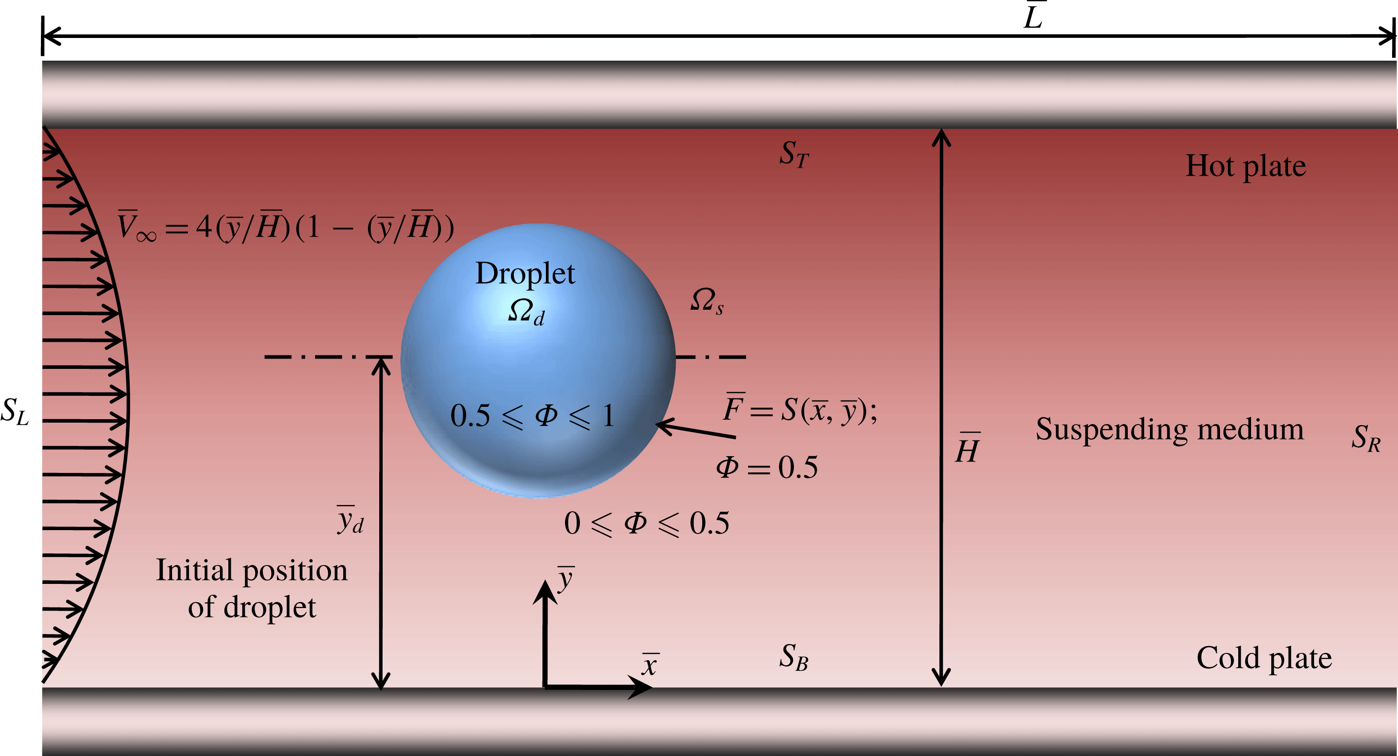
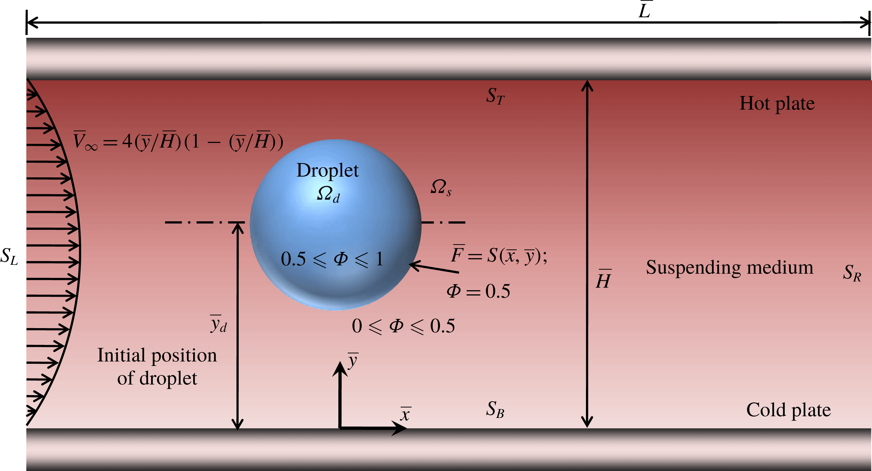
We first show a schematic of the numerical set-up in figure 2, where we have a Newtonian droplet suspended in another Newtonian fluid. The droplet is initially located at a distance
 $\bar{y}_{d}$
from the lower plate. The quantity
 $\unicode[STIX]{x1D6F7}$
is called the level set variable. It is constant at the interface and varies between
 $0.5$
and
 $1$
inside the droplet, whereas between
 $0.5$
and
 $1$
in the suspending phase. The upper plate is maintained at a higher temperature than the lower plate, with the distance between the two plates being
 $\bar{H}$
. The temperature is assumed to vary linearly in the transverse direction. The upper and lower boundaries (walls) of the computational domain are denoted by
 $S_{T}$
and
 $S_{B}$
respectively. A pressure driven flow is imposed in the microchannel at
 $S_{L}$
.
4.2 Governing equations and boundary conditions
We use the conservative level set approach to solve the two-phase flow. Details of this method are available in the literature (Sethian & Smereka Reference Sethian and Smereka2003; Olsson & Kreiss Reference Olsson and Kreiss2005; Nguyen & Chen Reference Nguyen and Chen2010; Balcázar, Oliva & Rigola Reference Balcázar, Oliva and Rigola2016). Here, we provide a brief overview of the methodology and the relevant governing equations to be solved. The entire domain consists of droplet and carrier phase subdomains,
 $(\unicode[STIX]{x1D6FA}_{d},\unicode[STIX]{x1D6FA}_{s})$
, as shown in figure 2. As per Olsson & Kreiss (Reference Olsson and Kreiss2005), the level set function,
 $\unicode[STIX]{x1D6F7}$
, varies smoothly from 0 to 1 across the interface. The droplet interface is located at
 $\unicode[STIX]{x1D6F7}=0.5$
. The level set function,
 $\unicode[STIX]{x1D6F7}$
, is assumed to vary in the two phases in the following manner:
 $0.5\leqslant \unicode[STIX]{x1D6F7}\leqslant 1$
in
 $\unicode[STIX]{x1D6FA}_{d}$
and
 $0\leqslant \unicode[STIX]{x1D6F7}\leqslant 0.5$
in
 $\unicode[STIX]{x1D6FA}_{s}$
. All of the governing equations as well as the corresponding boundary conditions are written in their dimensionless form using the dimensionless scheme described earlier in § 3.2.
Schematic of the numerical set-up consisting of a viscous Newtonian droplet immersed in a Newtonian carrier fluid within a parallel plate channel. The 2-D computational domain considered has a length and width of
 $\bar{L}$
and
 $\bar{H}$
respectively. The droplet domain is denoted by
 $\unicode[STIX]{x1D6FA}_{d}$
and the carrier phase domain by
 $\unicode[STIX]{x1D6FA}_{s}$
. The left and right boundaries
 $(S_{L},S_{R})$
of the computational domain are periodically connected. The droplet has a radius of
 $a$
and is placed at a position
 $\bar{y}_{d}$
from the bottom plate.
Here, we state the governing equations and boundary conditions that are used for the purpose of a full-scale numerical simulation. Thus, we do not consider any of the assumptions that were made in the previous section. The governing equation for
 $\unicode[STIX]{x1D6F7}$
, which signifies the reinitialized convection of the interface, is given by (Olsson & Kreiss Reference Olsson and Kreiss2005; Wang et al.
Reference Wang, Lu, Wang, Yang and Mao2008; Nguyen & Chen Reference Nguyen and Chen2010; Balcázar et al.
Reference Balcázar, Oliva and Rigola2016)
 $$\begin{eqnarray}\frac{\unicode[STIX]{x2202}\unicode[STIX]{x1D6F7}}{\unicode[STIX]{x2202}t}+\boldsymbol{u}\boldsymbol{\cdot }\unicode[STIX]{x1D735}\unicode[STIX]{x1D6F7}=\unicode[STIX]{x1D6FE}\unicode[STIX]{x1D735}\boldsymbol{\cdot }\left[\unicode[STIX]{x1D700}\unicode[STIX]{x1D735}\unicode[STIX]{x1D6F7}-\unicode[STIX]{x1D6F7}(1-\unicode[STIX]{x1D6F7})\frac{\unicode[STIX]{x1D735}\unicode[STIX]{x1D6F7}}{|\unicode[STIX]{x1D735}\unicode[STIX]{x1D6F7}|}\right],\end{eqnarray}$$
where
 $\unicode[STIX]{x1D6FE}(=\bar{\unicode[STIX]{x1D6FE}}/\bar{V}_{c})$
is the reinitialization parameter and
 $\unicode[STIX]{x1D700}(=\bar{\unicode[STIX]{x1D700}}/a)$
is the parameter governing interface thickness. The different fluid properties are expressed in terms of the level set function as follows:
 $$\begin{eqnarray}\left.\begin{array}{@{}c@{}}\displaystyle k=\unicode[STIX]{x1D6F7}k_{i}+(1-\unicode[STIX]{x1D6F7})k_{e},\\ \displaystyle \unicode[STIX]{x1D707}=\unicode[STIX]{x1D6F7}\unicode[STIX]{x1D707}_{i}+(1-\unicode[STIX]{x1D6F7})\unicode[STIX]{x1D707}_{e}.\end{array}\right\}\end{eqnarray}$$
In the numerical simulations, as we have considered a neutrally buoyant droplet, we can write
 $\unicode[STIX]{x1D70C}=\unicode[STIX]{x1D70C}_{i}=\unicode[STIX]{x1D70C}_{e}$
. The non-dimensional continuity and the Navier–Stokes equation are obtained by using the same non-dimensional scheme (as was used in the previous section) as in (2.1) and (2.2). Further substituting (4.2) into the dimensionless governing equations, we finally obtain
 $$\begin{eqnarray}\displaystyle \unicode[STIX]{x1D735}\boldsymbol{\cdot }\boldsymbol{u}=0, & & \displaystyle\end{eqnarray}$$
 $$\begin{eqnarray}\displaystyle Re\{\unicode[STIX]{x1D714}\unicode[STIX]{x1D6F7}+(1-\unicode[STIX]{x1D6F7})\}\left\{\frac{\unicode[STIX]{x2202}\boldsymbol{u}}{\unicode[STIX]{x2202}t}+\unicode[STIX]{x1D735}\boldsymbol{\cdot }(\boldsymbol{u}\boldsymbol{u})\right\} & = & \displaystyle -\unicode[STIX]{x1D735}p+\unicode[STIX]{x1D735}\boldsymbol{\cdot }[\{\unicode[STIX]{x1D706}\unicode[STIX]{x1D6F7}+(1-\unicode[STIX]{x1D6F7})\}\{\unicode[STIX]{x1D735}\boldsymbol{u}+(\unicode[STIX]{x1D735}\boldsymbol{u})^{\text{T}}\}]\nonumber\\ \displaystyle & & \displaystyle +\,\boldsymbol{F}_{st}+\boldsymbol{F}_{v},\end{eqnarray}$$
where
 $Re=\unicode[STIX]{x1D70C}_{e}\bar{V}_{c}H/\unicode[STIX]{x1D707}_{e}$
is the Reynolds number signifying the ratio of the inertia and viscous forces, and
 $\unicode[STIX]{x1D714}=\unicode[STIX]{x1D70C}_{i}/\unicode[STIX]{x1D70C}_{e}$
is the ratio of the density of the inner fluid to that of the outer fluid (
 $\unicode[STIX]{x1D714}=1$
for a neutrally buoyant droplet). We have considered the body forces in the governing equations to take into account the effect of the viscous as well as surface tension forces on the droplet dynamics. The term
 $\boldsymbol{F}_{v}=(8a^{2}/H^{2})\hat{\boldsymbol{x}}$
is the dimensionless volumetric force acting on the fluid due to the imposed pressure gradient and
 $\boldsymbol{F}_{st}=(\unicode[STIX]{x1D70E}/Ca)\unicode[STIX]{x1D705}\unicode[STIX]{x1D6FF}H^{2}\boldsymbol{n}$
is the non-dimensional surface tension force. Here,
 $\boldsymbol{n}=\unicode[STIX]{x1D735}\unicode[STIX]{x1D6F7}/|\unicode[STIX]{x1D735}\unicode[STIX]{x1D6F7}||_{\unicode[STIX]{x1D6F7}=0.5}$
is a unit vector representing the normal drawn on the droplet surface,
 $\unicode[STIX]{x1D705}$
is the local interfacial curvature, given by
 $$\begin{eqnarray}\unicode[STIX]{x1D705}=\unicode[STIX]{x1D735}\boldsymbol{\cdot }\boldsymbol{n},\end{eqnarray}$$
and
 $\unicode[STIX]{x1D6FF}=\unicode[STIX]{x1D6FF}(\unicode[STIX]{x1D6F7})$
is the Dirac delta function that ensures that
 $\boldsymbol{F}_{st}$
acts on the surface of the droplet,
 $F$
.
The non-dimensional energy equation for solving the temperature field, obtained from (2.3) and (4.2), is written as
 $$\begin{eqnarray}Pe_{T}\{\unicode[STIX]{x1D714}\unicode[STIX]{x1D6F7}+(1-\unicode[STIX]{x1D6F7})\}\left(\frac{\unicode[STIX]{x2202}T}{\unicode[STIX]{x2202}t}+\boldsymbol{u}\boldsymbol{\cdot }\unicode[STIX]{x1D735}T\right)=\unicode[STIX]{x1D735}\boldsymbol{\cdot }[\{\unicode[STIX]{x1D709}\unicode[STIX]{x1D6F7}+(1-\unicode[STIX]{x1D6F7})\}\unicode[STIX]{x1D735}T],\end{eqnarray}$$
where
 $Pe_{T}=\bar{V}_{c}a/\unicode[STIX]{x1D6FC}_{e}$
is the thermal Péclet number and
 $\unicode[STIX]{x1D6FC}_{e}=k_{e}/\unicode[STIX]{x1D70C}_{e}c_{p}$
is the thermal diffusivity of the carrier phase. The thermal conductivity is taken to be a constant in space and time. Moreover, any viscous dissipation or radiation from either of the phases is neglected.
Now, we state the dimensionless boundary conditions at the upper and lower plates,
 $S_{T}$
and
 $S_{B}$
(see figure 2) required to solve the above set of equations. We denote the unit vector normal to a wall (or plate) as
 $\boldsymbol{n}_{s}$
.
 $$\begin{eqnarray}\left.\begin{array}{@{}c@{}}\displaystyle \text{(i) No slip: }\boldsymbol{u}-(\boldsymbol{u}\boldsymbol{\cdot }\boldsymbol{n}_{s})\boldsymbol{n}_{s}=\mathbf{0}.\\ \displaystyle \text{(ii) No penetration: }\boldsymbol{u}\boldsymbol{\cdot }\boldsymbol{n}_{s}=0.\\ \displaystyle \text{(iii) No flux: }\boldsymbol{n}_{s}\boldsymbol{\cdot }\unicode[STIX]{x1D735}\unicode[STIX]{x1D6F7}=0.\end{array}\right\}\end{eqnarray}$$
Finally, the conditions required for the periodicity of the velocity and pressure fields as well as for the level set function at
 $S_{L}$
and
 $S_{R}$
are given by
 $$\begin{eqnarray}\left.\begin{array}{@{}c@{}}\displaystyle \text{(i) }\boldsymbol{u}(\boldsymbol{x})=\boldsymbol{u}(\boldsymbol{x}+L),\\ \displaystyle \text{(ii) }p(\boldsymbol{x})=p(\boldsymbol{x}+L),\\ \displaystyle \text{(iii) }\unicode[STIX]{x1D6F7}(\boldsymbol{x})=\unicode[STIX]{x1D6F7}(\boldsymbol{x}+L).\end{array}\right\}\end{eqnarray}$$
It can be seen that (4.1), (4.3), (4.4) and (4.6) are nonlinear coupled partial differential equations, which cannot be solved analytically. Therefore, we use the conservative level set approach to solve the flow field and the temperature field numerically.
In accordance with figure 2, we choose a 2-D rectangular computational domain of aspect ratio
 $3\times 1$
, tessellated with uniform grids. Equations (4.1), (4.3), (4.4) and (4.6) are solved along with the relevant boundary conditions, equations (4.7) and (4.8), using the finite-element-based conservative level set method with second-order Lagrangian triangular elements. The initial value of the level set function,
 $\unicode[STIX]{x1D6F7}$
, is taken as
 $$\begin{eqnarray}\left.\begin{array}{@{}c@{}}\displaystyle \text{carrier phase: }\unicode[STIX]{x1D6F7}(t=0)=0,\\ \displaystyle \text{droplet phase: }\unicode[STIX]{x1D6F7}(t=0)=1.\end{array}\right\}\end{eqnarray}$$
The initial velocity profile of the flow field is that of a plane Poiseuille flow and is given by
 $$\begin{eqnarray}\boldsymbol{u}(t=0)=\boldsymbol{V}_{\infty }=4\left(\frac{y}{H}\right)\left(1-\frac{y}{H}\right)\boldsymbol{e}_{x},\end{eqnarray}$$
where
 $\boldsymbol{e}_{x}$
is the unit vector in the
 $x$
direction. The initial temperatures of the upper and the lower plates are held constant and are taken to be
 $T_{L}=y_{min}$
and
 $T_{H}=y_{min}+H$
respectively, where
 $y_{min}$
is the position of the lower plate in the computational domain.
5 Results and discussion
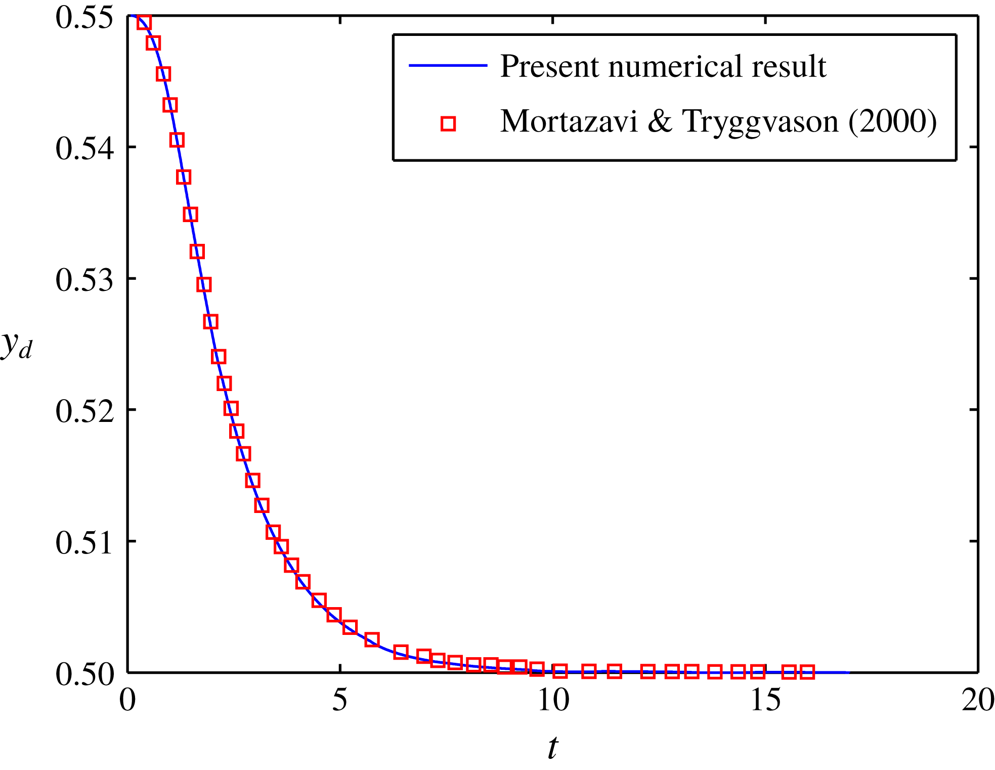
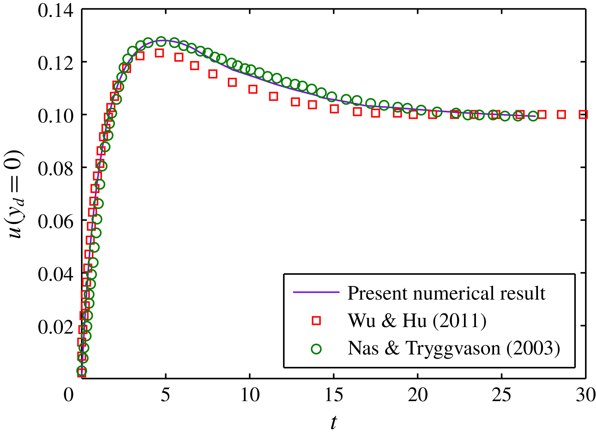
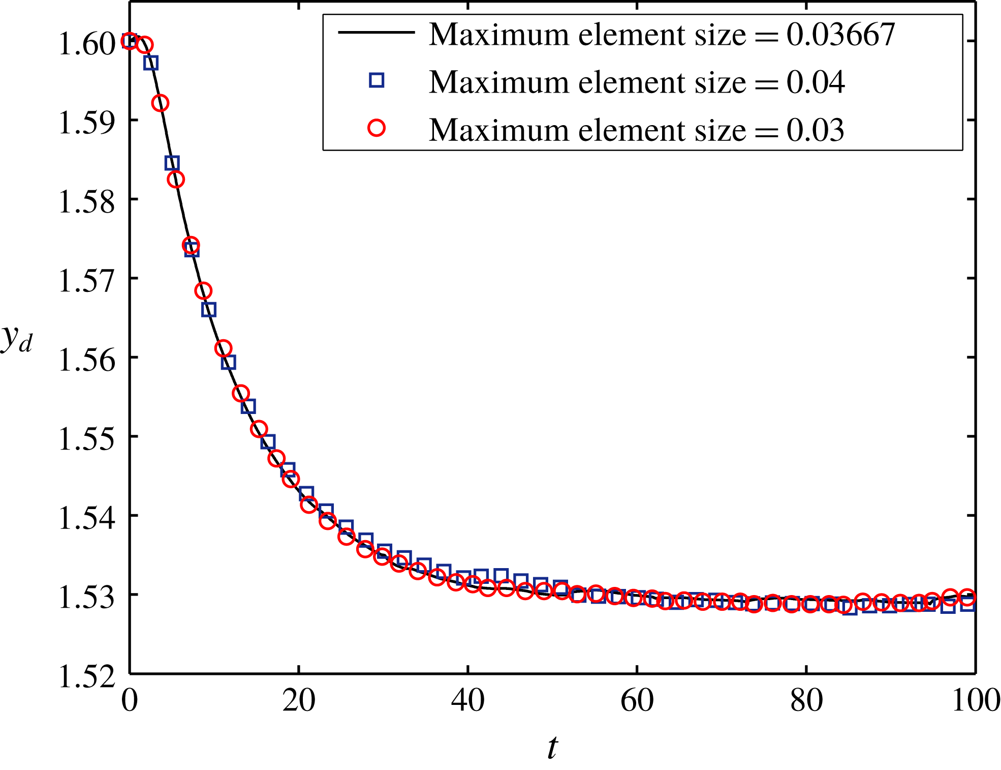
We first validate our numerical results with two previously published works. First, we match the temporal variation of the transverse position of the droplet with that obtained by Mortazavi & Tryggvason (Reference Mortazavi and Tryggvason2000). Second, we match the axial migration velocity of a droplet due to an imposed temperature gradient with that obtained by Nas & Tryggvason (Reference Nas and Tryggvason2003). The details of these validations are provided in appendix B. We also carry out a grid-independence check to ensure that our numerical results are not affected much by a change in the element size. The details of this check along with a plot showing the time variation of the transverse position of the droplet for different values of the maximum element size are provided in appendix C. We next compare our numerical and analytical results obtained in the present analysis.
5.1 Comparison between numerical and analytical results
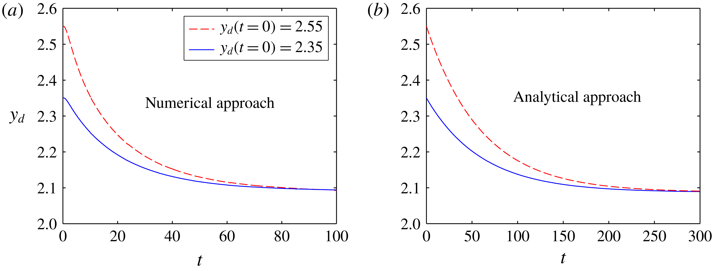
In this section, we provide a qualitative matching of the trend in the variation of the transverse position of the droplet with time. In figure 3(a), we show the temporal variation of the transverse position of the droplet for different initial positions
 $(y_{d}(t=0)=2.35,2.55)$
, obtained numerically. The confinement ratio of the system, which is the ratio of the droplet radius
 $(a)$
to the channel width
 $(\bar{H})$
, has been taken as 0.25 in order to obtain a good match with the theoretical results. The other parameters used in this simulation are
 $Re=0.001$
,
 $Ca=0.3$
,
 $Ma_{T}=0.001$
,
 $\unicode[STIX]{x1D706}=0.1$
and
 $\unicode[STIX]{x1D709}=1$
. The corresponding theoretical plot is shown in figure 3(b). We obtain this temporal variation of the transverse position of the droplet by substituting
 $U_{y}=\text{d}y_{d}/\text{d}t$
in the expression for the cross-stream migration velocity of the droplet, which is given by
 $$\begin{eqnarray}U_{y}=\text{d}y_{d}/\text{d}t=U_{y}^{(0)}+CaU_{y}^{(Ca)}+O(Ca^{2}),\end{eqnarray}$$
where the expression for
 $U_{y}^{(0)}$
is provided in the supplementary material and
 $U_{y}^{(Ca)}$
is given in (3.12). Thus, solving for
 $y_{d}(t)$
from the above equation, we obtain
 $$\begin{eqnarray}y_{d}(t)=\frac{\unicode[STIX]{x1D71B}}{\unicode[STIX]{x1D710}}+\left\{y_{d}(t=0)-\frac{\unicode[STIX]{x1D71B}}{\unicode[STIX]{x1D710}}\right\}\exp \left(-\frac{t}{\unicode[STIX]{x1D70F}_{c}}\right),\end{eqnarray}$$
where the expressions for the constants
 $\unicode[STIX]{x1D71B}$
and
 $\unicode[STIX]{x1D710}$
are given in appendix D. The term
 $\unicode[STIX]{x1D70F}_{c}(=1/\unicode[STIX]{x1D710})$
in the above expression represents the characteristic time constant. As can be seen, there is a good qualitative match between the two plots.
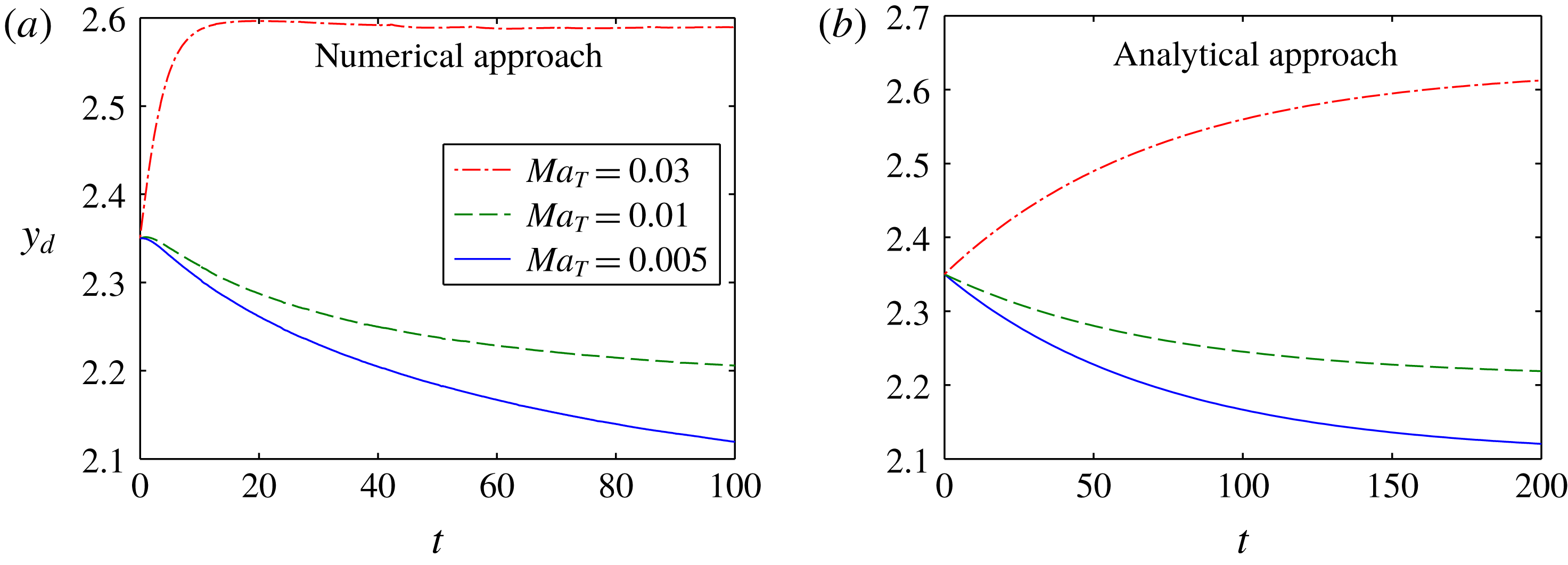
Next, we also show a qualitative match of the variation of the transverse position of the droplet with time for different values of
 $Ma_{T}~(0.005,0.01,0.03)$
in figure 4. In figure 4(a), we show the numerical results, with the other parameters being the same as in figure 3. A theoretical plot is also displayed for the same values of
 $Ma_{T}$
in figure 4(b). Although we do not have an exact match, the trend of cross-stream migration of the droplet remains the same.
Variation of the transverse position of the droplet with time for different initial positions,
 $y_{d}(t=0)=2.35$
, 2.55. (a) Numerically obtained result using the conservative level set method. The channel dimensions are
 $4\times 12$
. (b) Analytically obtained result. The constant parameter values are
 $Ca=0.3$
,
 $\unicode[STIX]{x1D714}=\unicode[STIX]{x1D709}=1$
,
 $\unicode[STIX]{x1D706}=0.1$
,
 $Ma_{T}=0.001$
,
 $Re=0.001$
and
 $H=4$
.

Temporal variation of the transverse position of the droplet for different values of the Marangoni number,
 $Ma_{T}=0.005$
, 0.01, 0.03. (a) Numerically obtained result using the conservative level set method. The channel dimensions are
 $4\times 12$
. (b) Analytically obtained result. The various parameters involved for both of the plots are
 $Ca=0.3$
,
 $Re=0.001$
,
 $\unicode[STIX]{x1D714}=\unicode[STIX]{x1D709}=1$
,
 $\unicode[STIX]{x1D706}=0.1$
and
 $H=4$
.

For instance, in both of the cases, the droplet migrates towards the channel centreline and reaches a steady state subsequently, provided that
 $Ma_{T}<0.01$
. However, for
 $Ma_{T}=0.03$
, the droplet is always found to migrate away from the channel centreline. A detailed physical reasoning for such a behaviour is provided in the succeeding sections.
The comparison between the analytical and numerical results shows only qualitative agreement. The main reason for the quantitative disagreement is the presence of walls in the numerical simulation. Walls not only affect the flow field but also affect the distribution of temperature. Walls modify the hydrodynamic flow and thereby lead to a hydrodynamic lift force in the direction normal to the wall (Uijttewaal, Nijhof & Heethaar Reference Uijttewaal, Nijhof and Heethaar1993; Uijttewaal & Nijhof Reference Uijttewaal and Nijhof1995). This wall-induced lift force augments the droplet migration in Poiseuille flow also and the droplet reaches the steady-state transverse position much faster compared with the unbounded analytical result. A droplet positioned at some off-centreline location also encounters a different kind of temperature gradient due to the asymmetry in the distance from the walls. This asymmetry in the temperature gradient can affect the droplet migration. These effects are not taken into account in the analytical solution. Additionally, we have compared the results obtained from the 2-D numerical simulation with the 3-D analytical solution. To reduce the computational cost, we have restricted our work to 2-D simulations. A 3-D numerical simulation is expected to give better quantitative agreement. However, needless to say, 2-D simulations capture the essential physics of interest, as previously demonstrated by Mortazavi & Tryggvason (Reference Mortazavi and Tryggvason2000) and Stan et al. (Reference Stan, Guglielmini, Ellerbee, Caviezel, Stone and Whitesides2011).
5.2 Effect of
$Ca$
and
$Ma_{T}$
on cross-stream migration


We now explore the variation of the transverse position of the droplet with time. We run full-scale simulations for different values of
 $Ca$
and
 $Ma_{T}$
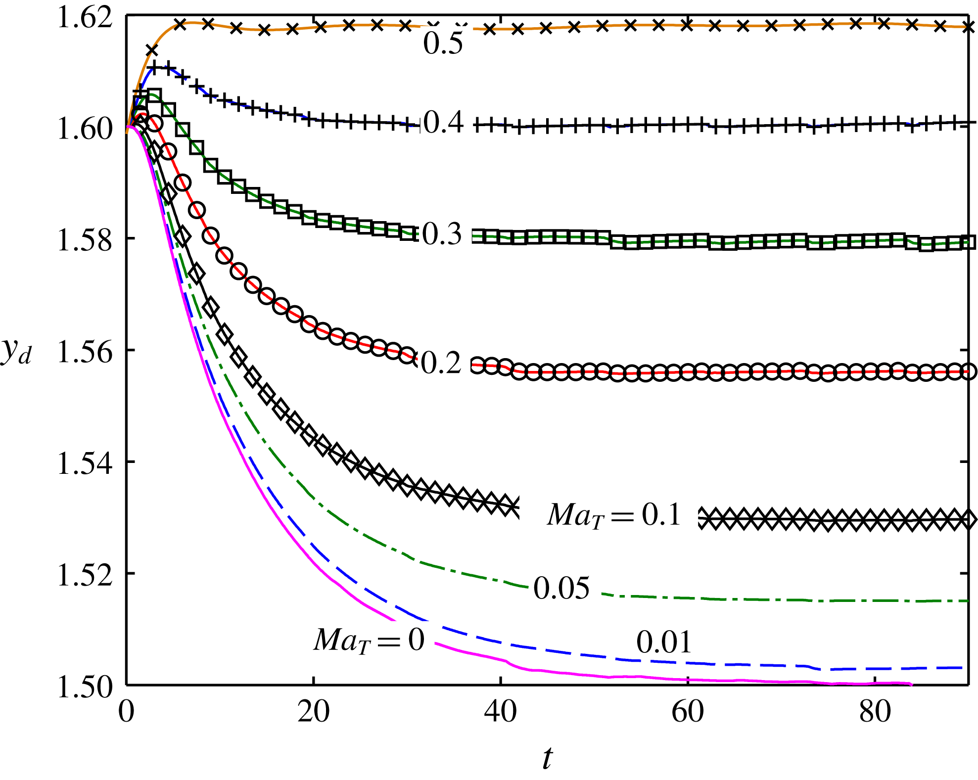
. In figure 5, we show the effect of
 $Ma_{T}$
on the cross-stream migration of a droplet for a constant value of
 $Ca$
. The other parameters used in these simulations are
 $Re=4$
,
 $Pe_{T}=20$
,
 $H=3$
and
 $L=9.$
It can be observed from figure 5 that increase in
 $Ma_{T}$
and hence increase in the thermal Marangoni stress shifts the steady-state position of the droplet further away from the channel centreline.
A proper justification for the nature of the temporal variation of the droplet transverse position can be given. We first discuss the hydrodynamics of the droplet suspended in an isothermal flow. The droplet, as seen from the schematics in figures 1 and 2, is placed at an off-centre position with respect to the centreline. At this off-centre position, the droplet shape becomes asymmetric due to the background Poiseuille flow. This asymmetric droplet shape is associated with streamlines that are asymmetric about the axial plane (Leal Reference Leal1980). As a result, even in the absence of any temperature gradient in the far field, a hydrodynamic force acts on the droplet, which forces it to migrate towards the centreline of the channel. However, in the presence of a transverse temperature gradient, as shown in figure 2, the droplet may migrate towards or away from the centreline together with an increase or decrease in the magnitude of its cross-stream migration velocity depending on the strength of the temperature field, which is manifested by the thermal Marangoni stress or the tangential stress jump at the droplet interface. This Marangoni stress is generated due to variation of surface tension forces along the droplet surface. For the present scenario, a higher temperature at the top plate indicates a lower surface tension along the upper hemisphere of the droplet compared with the lower hemisphere. Thus, the Marangoni stress forces the droplet to migrate towards the upper hot plate and as a result opposes the hydrodynamic force due to the imposed flow and shape deformation. With increase in the applied temperature gradient or the Marangoni stress, the net force acting on the droplet reduces and hence the cross-stream migration velocity decreases as well. Thus, as
 $Ma_{T}$
increases, the steady-state transverse position of the droplet gradually gets shifted away from the centreline of flow. Finally, a point is reached where the thermal Marangoni stress overcomes the hydrodynamic force and the droplet migrates away from the centreline of the channel.
Temporal evolution of the transverse position of the droplet for different values of
 $Ma_{T}$
. The other parameter values, which are maintained constant throughout these simulations, are
 $Ca=0.3$
,
 $Re=4$
,
 $\unicode[STIX]{x1D714}=\unicode[STIX]{x1D709}=1$
,
 $Pe_{T}=20$
,
 $H=3$
,
 $L=9$
.

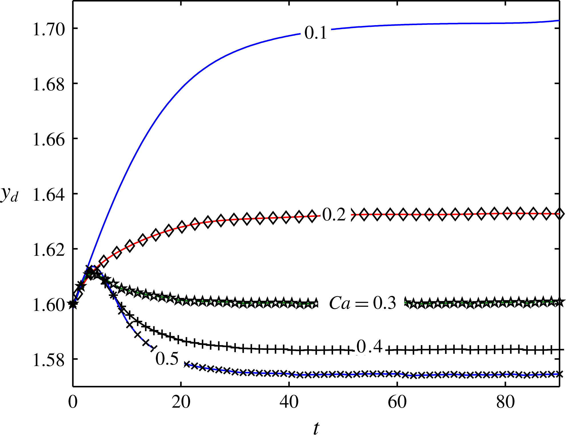
In figure 6, we show the effect of
 $Ca$
or shape deformation on the transverse migration of the droplet, for a constant value of
 $Ma_{T}$
. It is seen that the higher the value of
 $Ca$
is, the higher the effect of the hydrodynamic force due to the imposed flow is. It can be observed from figure 6 that the droplet migrates towards the upper plate of the channel for
 $Ma_{T}=0.4$
and
 $Ca=0.1$
. However, for
 $Ca=0.5$
, the droplet migrates towards the channel centreline for the same value of
 $Ma_{T}$
.
An appropriate physical explanation for this behaviour can be provided if we first look into the dynamics of a droplet in an isothermal flow field, which was previously studied by Chan & Leal (Reference Chan and Leal1979). In an isothermal flow field, the presence of droplet deformation results in an asymmetry in its shape about the channel centreline, which in turn results in streamlines asymmetric about the axial plane of the droplet. This asymmetry generates a hydrodynamic force that drives the droplet towards the flow centreline. Now, the presence of a transverse temperature gradient, as shown in figures 1 and 2, tends to drive the droplet from the lower plate to the upper hot plate. Thus, the thermally induced Marangoni stress opposes the shape-deformation-induced hydrodynamic force.
Temporal variation of the transverse position of the droplet for different values of
 $Ca$
. The other parameter values used are
 $Ma_{T}=0.4$
,
 $Re=4$
,
 $\unicode[STIX]{x1D714}=\unicode[STIX]{x1D709}=\unicode[STIX]{x1D706}=1$
,
 $Pe_{T}=20$
,
 $H=3$
and
 $L=9$
. The droplet is initially positioned above the channel centreline with
 $y_{d}(t=0)=1.6$
.

Initially, for a low value of
 $Ca(=0.1)$
, that is lower droplet deformation and hence lower hydrodynamic force, the thermal Marangoni stress dominates in driving the droplet towards the upper plate. However, increase in
 $Ca$
results in a higher hydrodynamic force, which, beyond a certain point
 $(Ca=0.24)$
, dominates the thermal Marangoni stress, resulting in a cross-stream migration of the droplet towards the channel centreline. This can clearly be observed from figure 6. From a mathematical perspective, the
 $O(Ca)$
droplet migration velocity components can be expressed as follows:
 $$\begin{eqnarray}\left.\begin{array}{@{}c@{}}\displaystyle U_{x}^{(Ca)}=\frac{6}{5}\frac{(3\unicode[STIX]{x1D706}\unicode[STIX]{x1D6FF}-21\unicode[STIX]{x1D706}+17\unicode[STIX]{x1D6FF}+16)Ma_{T}}{(\unicode[STIX]{x1D6FF}+2)^{2}(3\unicode[STIX]{x1D706}+2)^{2}}L_{2,1}^{(Ca)},\quad U_{y}^{(Ca)}=\aleph _{1}(L_{3,0}^{(Ca)}-10L_{3,2}^{(Ca)})+\aleph _{2}L_{2,1}^{(Ca)},\\ \displaystyle \text{where}\quad \aleph _{1}=\frac{4}{7}\frac{(3\unicode[STIX]{x1D706}^{2}-\unicode[STIX]{x1D706}+8)(-2e+H)}{H^{2}(\unicode[STIX]{x1D706}+1)(3\unicode[STIX]{x1D706}+2)},\quad \aleph _{2}=-\frac{16}{7}\frac{24\unicode[STIX]{x1D706}^{2}+49\unicode[STIX]{x1D706}-13}{(\unicode[STIX]{x1D706}+4)H^{2}(3\unicode[STIX]{x1D706}+2)^{2}}.\end{array}\right\}\qquad\end{eqnarray}$$
This clearly proves the strong dependence of the droplet cross-stream migration velocity on the shape deformation.
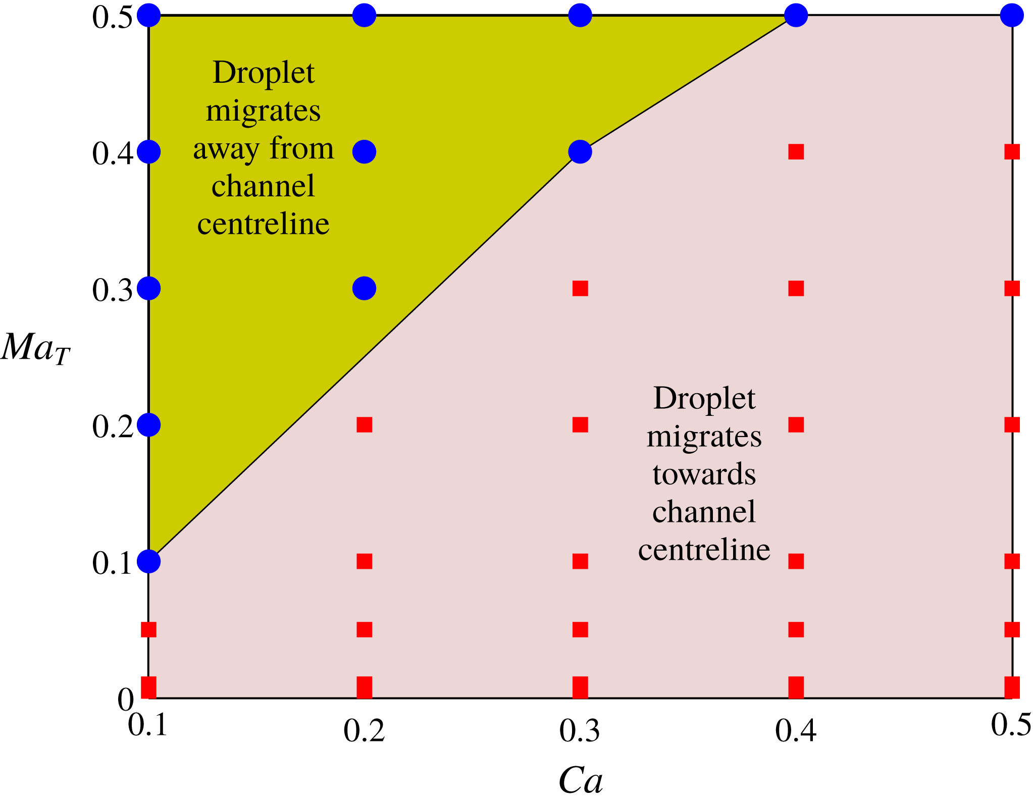
Next, we construct a regime diagram to show the droplet trajectory for different values of
 $Ca$
and
 $Ma_{T}$
. Figure 7 shows two distinguishable regimes: one of them indicates that the droplet migrates towards the centreline of the channel and the other signifies that the droplet moves towards the channel wall. The ‘red square’ data points indicate the values of
 $(Ca,Ma_{T})$
in the simulations that result in droplet migration towards the channel centreline, while the ‘blue circle’ data points represent the data points where the droplet migrates towards the wall (upper plate for the present case). The ‘green’ region signifies the regime where the droplet migrates towards the wall, whereas the ‘pink’ region indicates droplet migration towards the channel centreline.
Regime diagram showing the two separate regions of droplet migration. The other parameters are
 $Re=4$
,
 $Pe_{T}=20$
,
 $H=3$
and
 $L=9$
.

The borderline separating the two regimes represents the magnitude of the critical Marangoni number, which is the Marangoni number corresponding to zero cross-stream migration of the droplet. It should be noted that in addition to the hydrodynamic force due to the imposed flow as well as that due to shape deformation of the droplet, there exists another thermocapillary force in a non-isothermal flow field that drives the droplet towards the hotter region. This thermocapillary force is a manifestation of the Marangoni stress generated due to the variation of surface tension along the surface of the droplet. As per the schematic shown in figure 2, the droplet migrates towards the upper (hotter) plate, whereas the hydrodynamic force tends to move the droplet towards the channel centreline. Hence, the two forces oppose one another and the fate of the droplet dynamics depends on which of these effects dominates. However, for the special case where the effect due to the thermal Marangoni stress is exactly balanced by that due to the hydrodynamic force, a critical point is attained and there ceases to be any cross-stream migration of the droplet. The corresponding thermal Marangoni number is the critical Marangoni number and is denoted by
 $Ma_{T,cr}$
, the expression of which obtained from the condition of zero cross-stream migration velocity is
 $$\begin{eqnarray}\displaystyle & & \displaystyle Ma_{T,cr}=-\frac{4}{105\unicode[STIX]{x1D701}}\nonumber\\ \displaystyle & & \displaystyle \quad \times \,\frac{Ca(H-2y_{d})(198\unicode[STIX]{x1D706}^{5}-1242\unicode[STIX]{x1D706}^{4}-7327\unicode[STIX]{x1D706}^{3}-6292\unicode[STIX]{x1D706}^{2}+1843\unicode[STIX]{x1D706}+2320)(\unicode[STIX]{x1D709}+2)}{H^{4}(\unicode[STIX]{x1D706}+1)^{2}(2+3\unicode[STIX]{x1D706})(\unicode[STIX]{x1D706}+4)}.\nonumber\\ \displaystyle & & \displaystyle\end{eqnarray}$$
The above expression as well as figure 6 indicates that the magnitude of
 $Ma_{T,cr}$
increases with increase in
 $Ca$
. This behaviour can be explained as follows. A higher value for
 $Ca$
signifies larger droplet deformation and hence a higher hydrodynamic force which tends to drive the droplet towards the flow centreline. To neutralize this hydrodynamic force, hence, a larger Marangoni stress needs to be generated, which explains the increase in magnitude of
 $Ma_{T,cr}$
.
5.3 Effect of initial droplet position,
$y_{d}(t=0)$

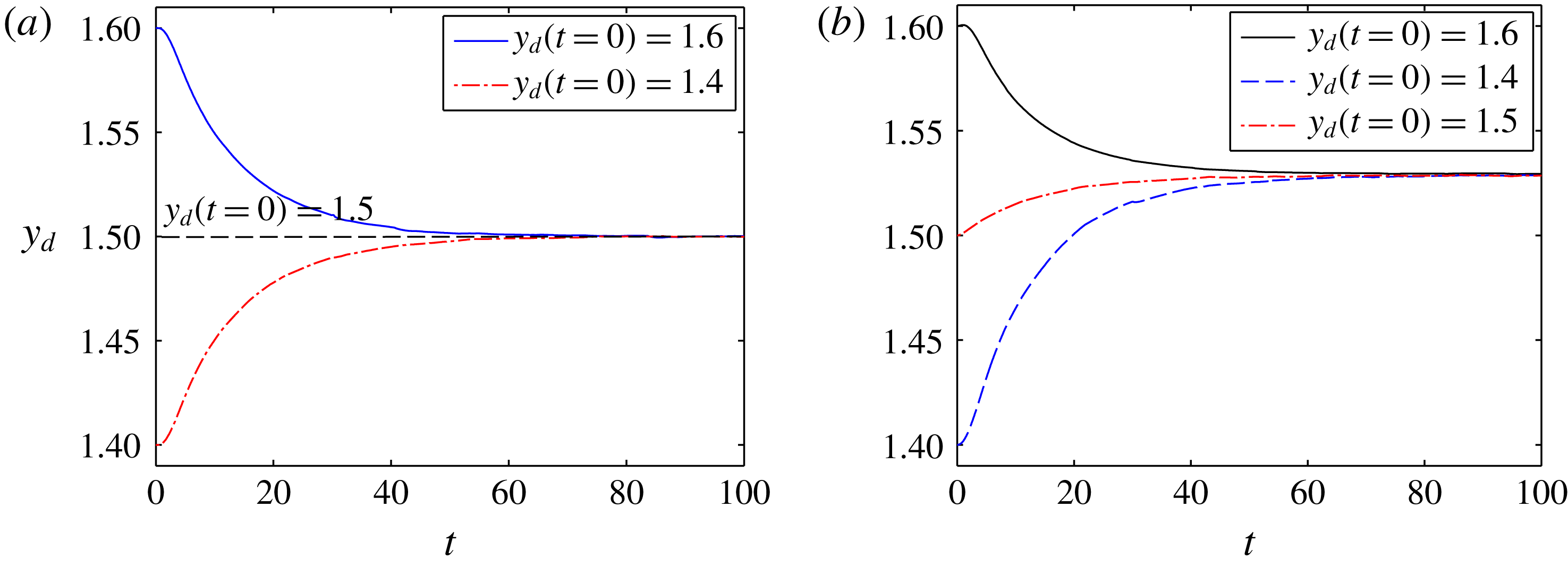
Now, we explore the possible effects of change in initial position of the droplet on its transverse migration. We first show, in figure 8(a), the temporal variation of the transverse position of the droplet for different initial positions of the droplet, above, below and on the centreline
 $(y_{d}(t=0)=1.4,1.5,1.6)$
, when suspended in an isothermal Poiseuille flow field
 $(Ma_{T}=0)$
. We see that when the droplet is initially placed on the channel axis
 $(y_{d}=H/2)$
, it migrates solely in the axial direction. However, when the droplet is eccentrically placed (
 $y_{d}(t=0)=1.4$
or 1.6), it always migrates towards the centreline of the channel, and the steady-state transverse position of the droplet becomes the channel centreline
 $(y_{d}(t=100)=H/2)$
itself. This behaviour of the droplet can be attributed to the hydrodynamic force induced due to the shape deformation of the droplet.
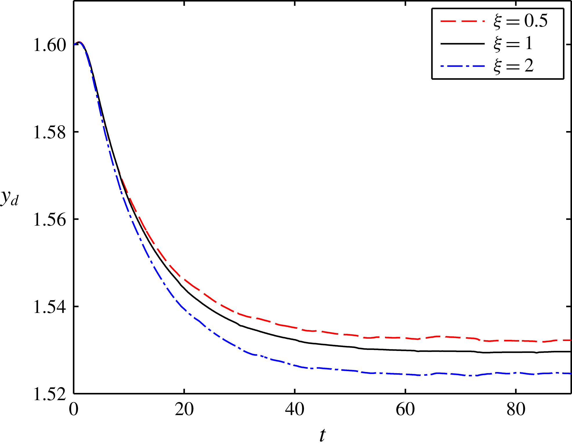
In figure 8(b), we consider a constant temperature gradient in the transverse direction. Under the effect of a linearly varying temperature field, the steady-state transverse position of the droplet no longer remains the channel centreline. Since the upper plate is the hotter one, the thermocapillary effect or the temperature-induced Marangoni stress causes the droplet to migrate upwards. The presence of hydrodynamic force induced by both the imposed flow and shape deformation, however, prevents the droplet from following a vertical path, as seen from figure 8(b). Depending on the initial position of the droplet as well as the dominating factor out of (i) the hydrodynamic force acting on the droplet due to the imposed Poiseuille flow and flow-induced-shape deformation (governed by
 $Ca$
), and (ii) the thermal Marangoni stress generated due to variation of the interfacial temperature (governed by
 $Ma_{T}$
), the droplet may migrate towards or away from the channel centreline. Whatever may be the case, the droplet always migrates to the same steady-state position, irrespective of the initial position of the droplet, for any constant values of
 $Ca$
and
 $Ma_{T}$
. This is a clear indication of the fact that the steady-state transverse position of the droplet is independent of the initial position of the droplet, which is due to the constancy of the two governing parameters
 $(Ca,Ma_{T})$
responsible for deciding the fate of the droplet. This steady-state position of the droplet may
 $(y_{d}=H/2)$
or may not
 $(y_{d}\neq H/2)$
be on the channel centreline depending on whether
 $Ma_{T}=0$
or
 $Ma_{T}\neq 0$
respectively. For the plot shown in figure 8(b), we have
 $Ma_{T}=0.1$
and
 $Ca=0.3$
, where the droplet reaches a steady-state position
 $y_{d}=1.528$
that is above the channel centreline.
Temporal variation of the transverse position of the droplet for different initial positions,
 $y_{d}(t=0)=1.4$
, 1.5, 1.6, in (a) an isothermal Poiseuille flow field
 $(Ma_{T}=0)$
and (b) a non-isothermal Poiseuille flow field
 $(Ma_{T}=0.1)$
. The other parameters, which are kept constant in these simulations, are
 $\unicode[STIX]{x1D714}=\unicode[STIX]{x1D709}=1$
,
 $Re=4$
,
 $Pe_{T}=20$
,
 $a/\bar{H}=0.33$
,
 $Ca=0.3$
.

5.4 Effect of confinement ratio,
$a/\bar{H}$

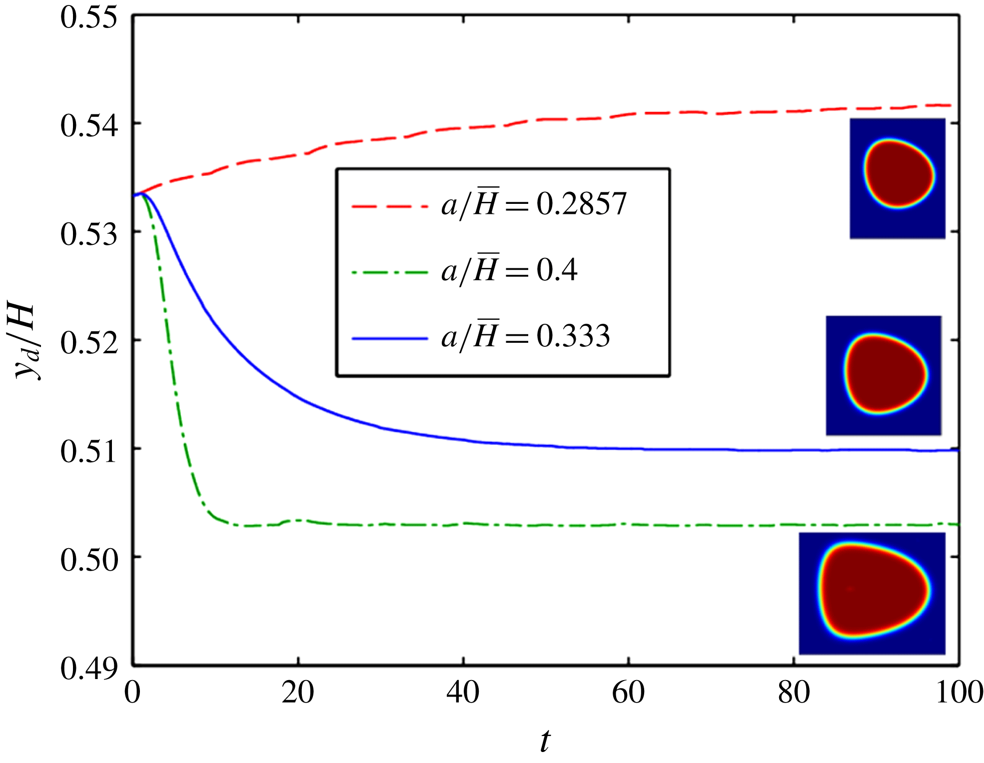
Now, we look into the effect of the confinement ratio on the droplet cross-stream migration. As seen from figure 9, the droplet migrates towards the channel centreline and reaches its steady-state position faster for a system with higher confinement ratio. As the confinement ratio decreases, the time taken by the droplet to reach the steady-state position increases. Moreover, the steady-state position of the droplet is shifted further away from the channel centreline for a lower confinement ratio. On further reduction of the confinement ratio
 $(a/\bar{H}=0.2857)$
, the droplet migrates away from the channel centreline.
A proper reasoning for this can be given as follows. When the confinement ratio is large or the droplet is larger than the channel width, the difference in the surface velocity on the droplet interface between the upper and lower hemispheres, due to the effect of imposed Poiseuille flow, is larger compared with a system with low confinement ratio. Hence, the droplet deformation is enhanced for a system with a higher
 $a/\bar{H}$
value (as can be seen from the insets in figure 9), which results in a larger hydrodynamic force on the droplet. This hydrodynamic force that drives the droplet towards the channel centreline is opposed by the thermal Marangoni stress. With a gradual increase in
 $a/\bar{H}$
, the hydrodynamic force finally overpowers the thermocapillary effect, and the droplet, which initially migrated away from the channel centreline for low values of
 $a/\bar{H}(=0.2857)$
, now starts to migrate towards it for higher values of
 $a/\bar{H}(=0.4)$
.
Variation of the transverse position of the droplet (normalized with channel height) with time for different values of the confinement ratio
 $a/\bar{H}=0.2857$
, 0.333, 0.4. The droplet shape for each confinement ratio at
 $t=100$
is shown as an inset. The other parameters are
 $\unicode[STIX]{x1D714}=\unicode[STIX]{x1D709}=\unicode[STIX]{x1D706}=1$
,
 $Re=4$
,
 $Pe_{T}=20$
,
 $Ca=0.3$
,
 $Ma_{T}=0.1$
. The initial position of the droplet for all three cases is taken as
 $y_{d}(t=0)=1.6$
.

A higher value of
 $a/\bar{H}$
hence indicates a larger cross-stream migration velocity, which causes the droplet to reach its steady-state position quickly and also closer to the channel centreline. A smaller value of
 $a/\bar{H}$
, on the contrary, leads to a reduced gradient of the surface velocity along the interface. This indicates a higher thermocapillary effect, and the steady-state transverse position of the droplet drifts further away from the channel centreline. The different steady-state droplet shapes at
 $t=100$
for different values of
 $a/\bar{H}$
are highlighted in the insets of figure 9. It is seen from the figure that the droplet deforms most for the highest confinement ratio
 $(a/\bar{H}=0.4)$
due to the strong effect of the imposed flow. The droplet for this case is found to be stretched in the axial direction with a sharp leading edge and a flat trailing edge. The deformation of the droplet is minimum for
 $a/\bar{H}=0.2875$
. All of the other parameters,
 $Ca$
,
 $Ma_{T}$
,
 $Pe_{T}$
,
 $\unicode[STIX]{x1D709}$
,
 $\unicode[STIX]{x1D714}$
,
 $\unicode[STIX]{x1D706}$
, as well as the initial position of the droplet, are kept constant.
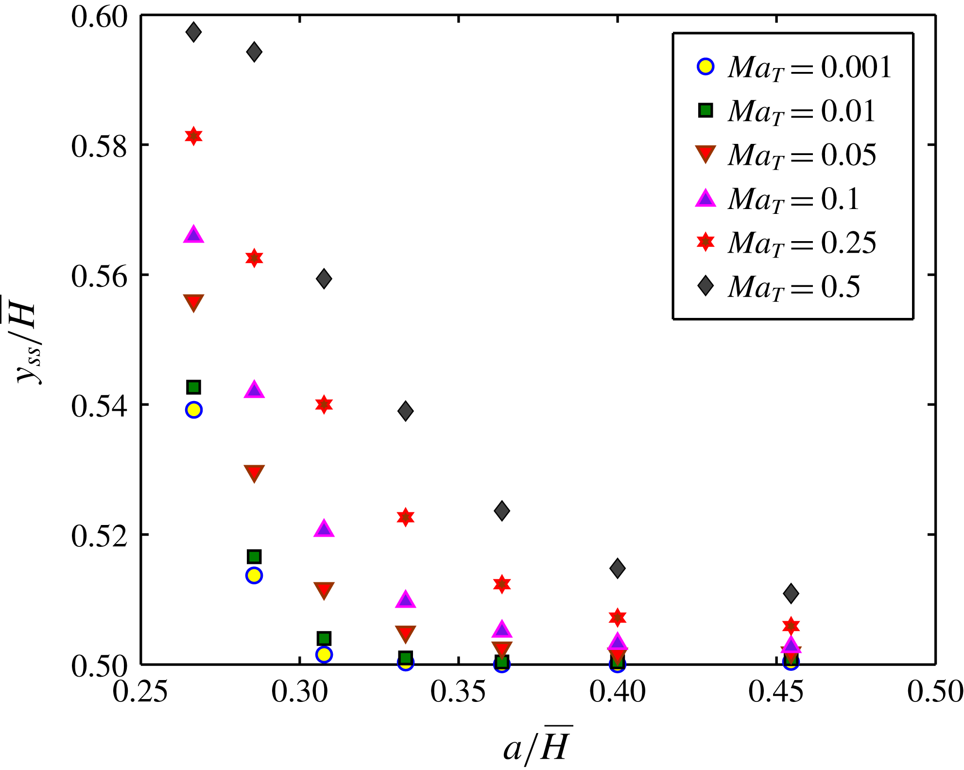
Variation of the steady-state transverse position of the droplet (normalized with channel height) as a function of the confinement ratio,
 $a/\bar{H}$
, for different values of
 $Ma_{T}$
. The other parameters are
 $\unicode[STIX]{x1D714}=\unicode[STIX]{x1D709}=\unicode[STIX]{x1D706}=1$
,
 $Re=4$
,
 $Pe_{T}=20$
,
 $Ca=0.3$
. The normalized initial position of the droplet for all cases is taken as
 $y_{d}(t=0)/\bar{H}=0.53$
.

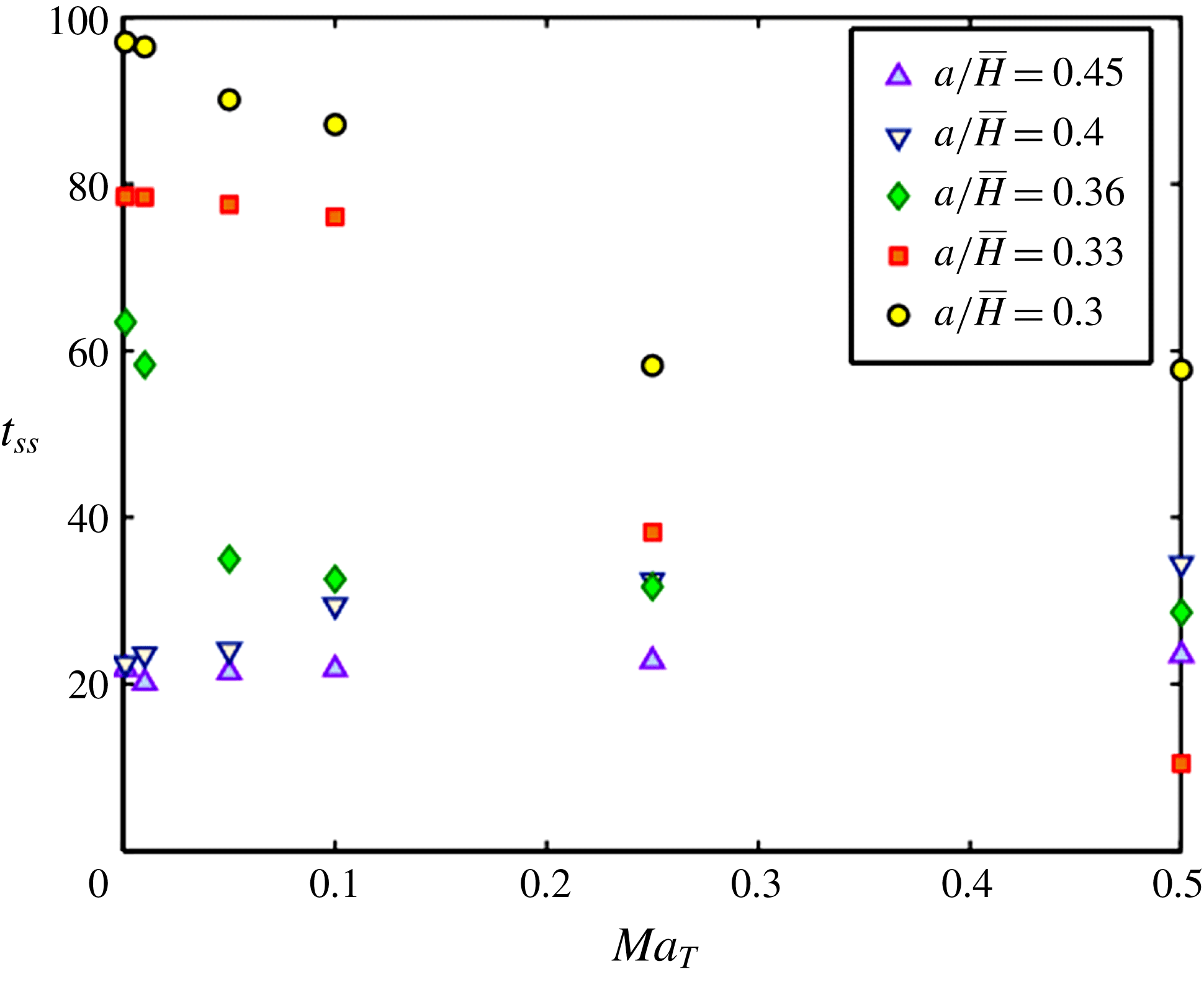
Variation of the time required to reach a steady-state transverse position with
 $Ma_{T}$
for different values of the confinement ratio
 $a/\bar{H}$
. The other parameters are
 $\unicode[STIX]{x1D714}=\unicode[STIX]{x1D709}=\unicode[STIX]{x1D706}=1$
,
 $Re=4$
,
 $Pe_{T}=20$
,
 $Ca=0.3$
. The normalized initial position of the droplet for all three cases is taken as
 $y_{d}(t=0)/\bar{H}=0.53$
.

We next show the variation of the normalized steady-state transverse position
 $(y_{ss}/\bar{H})$
of the droplet as a function of the confinement ratio for different values of the applied temperature gradient (or
 $Ma_{T}$
) in figure 10. The values of the different parameters used in the numerical simulation are stated in the caption. As already explained, it can be observed from figure 10 that the steady-state transverse position of the droplet shifts closer to the channel centreline with increase in
 $a/\bar{H}$
for a constant imposed temperature gradient (or
 $Ma_{T}$
). For a sufficiently lower confinement ratio, the droplet settles down at a position far away from the channel centreline. Figure 10 provides evidence that both the confinement ratio and the applied temperature gradient play important roles in altering the steady-state transverse position of the droplet. For higher values of
 $Ma_{T}$
, variation in
 $a/\bar{H}$
plays an important role in relocating the droplet compared with lower values of
 $Ma_{T}$
. This is due to the fact that a higher temperature gradient (or
 $Ma_{T}$
) provides wider scope for variation in the steady-state position of the droplet due to change in
 $a/\bar{H}$
. On the contrary, for lower values of
 $Ma_{T}$
, the thermocapillary force becomes insufficient to drive the droplet away from the channel centreline, resulting in its settling down in the vicinity of the centreline, even for a larger channel height (or low
 $a/\bar{H}$
). Another important fact that is evident from figure 10 is the important role of
 $a/\bar{H}$
. For lower confinement ratios, droplet deformation, induced by the imposed flow, decreases, which results in a reduced hydrodynamic force. Thus, the dominating effect of the thermal Marangoni stress, under such a scenario, is highly effective in driving the droplet towards the wall compared with the case with a higher value of
 $a/\bar{H}$
.
We also investigate the role of the confinement ratio on the time needed to reach the steady-state position
 $(t_{ss})$
of the droplet in figure 11. It can be noted from the figure that for a constant temperature gradient, increase in the confinement ratio reduces the time taken by the droplet to reach its steady-state position
 $(t_{ss})$
. In addition, it is also observed that the same effect of the confinement ratio is rather enhanced for low values of
 $Ma_{T}$
. On the other hand, increase in
 $Ma_{T}$
significantly reduces
 $t_{ss}$
too, provided that the value of
 $a/\bar{H}$
is low enough. A proper explanation for the above observations can be given if we look into the net force acting on the droplet. In general, increase in the confinement ratio enhances the imposed flow-induced shape deformation of the droplet, which in turn results in a higher hydrodynamic force directed towards the channel centreline. In other words, a large value of
 $a/\bar{H}$
is accompanied by a higher cross-stream migration velocity and hence a shorter time to reach the steady-state position of the droplet. The important factor responsible for controlling this time,
 $t_{ss}$
, is the magnitude of the net force acting on the droplet that drives it towards the channel centreline or away from it. The larger this net force is, the shorter the time the droplet will take to reach its steady state. Hence, for the case when there is a minimal effect of the applied temperature gradient
 $(Ma_{T}\rightarrow 0)$
, increase in
 $a/\bar{H}$
results in a greater fall in
 $t_{ss}$
compared with the case of large
 $Ma_{T}$
, even though
 $a/\bar{H}$
is varied through the same range. For larger values of
 $a/\bar{H}$
, the resulting hydrodynamic force acting on the droplet is large enough to dominate any effect of the applied temperature gradient. Hence,
 $t_{ss}$
almost remains constant for a fixed
 $a/\bar{H}$
even though there is a variation in
 $Ma_{T}$
, provided that the magnitude of
 $a/\bar{H}$
is high enough. For lower values of
 $a/\bar{H}$
, both the thermocapillary force and the hydrodynamic force are of comparable magnitude. However, increase in
 $Ma_{T}$
results in an increase in the net force acting on the droplet, as a consequence of which the droplet reaches its steady state more quickly (
 $t_{ss}$
decreases). All of this is evident from figure 11.
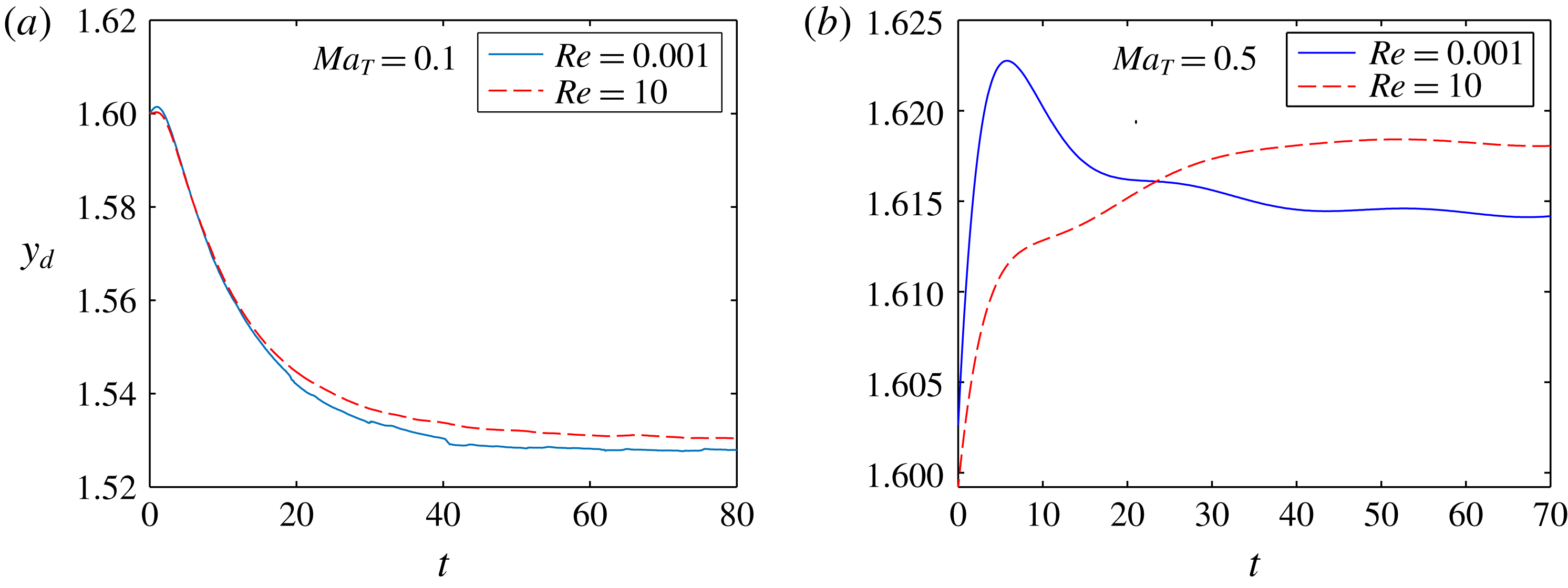
Variation of the transverse position of the droplet as a function of time for different values of
 $Re$
. In (a),
 $Ma_{T}=0.1$
, whereas in (b),
 $Ma_{T}=0.5$
. The other parameters used in the numerical simulations are
 $\unicode[STIX]{x1D714}=\unicode[STIX]{x1D706}=\unicode[STIX]{x1D709}=1$
,
 $Ca=0.3$
,
 $a/\bar{H}=0.333$
,
 $Pe_{T}=20$
and
 $y_{d}(t=0)=1.6$
.

5.5 Effect of inertia in fluid flow
We next analyse the effect of inertia on the dynamics of the droplet as well as its steady-state transverse position. For this, we have plotted the temporal variation of the transverse position of the droplet for different values of
 $Re$
in figure 12. It can be seen from both figures 12(a) and 12(b) that increase in fluid inertia (manifested by an increase in
 $Re$
) is accompanied by a shift of the steady-state transverse position of the droplet away from the channel centreline. The effect of fluid inertia is enhanced with increase in the applied temperature gradient
 $(Ma_{T})$
. The implication of this is that the steady-state position of the droplet is seen to be shifted towards the wall by a greater extent for
 $Ma_{T}=0.5$
compared with the case for
 $Ma_{T}=0.1$
for the same increase in
 $Re$
. A physical explanation for this behaviour of the droplet can be provided if we look into the inertial lift that acts on the droplet at finite values of
 $Re$
. In general, inertial lift may be of two types. The first is the so-called ‘wall effect’ generated due to the presence of an asymmetric wake created by the droplet near the wall. This produces a lift force that pushes the droplet towards the channel centreline. The second is the inertial lift induced by a shear gradient in the flow field which forces the droplet to migrate towards regions of high shear rate, that is, near the channel walls (Di Carlo et al.
Reference Di Carlo, Irimia, Tompkins and Toner2007; Stan et al.
Reference Stan, Guglielmini, Ellerbee, Caviezel, Stone and Whitesides2011). For the present scenario, the second one is the dominant lift force that acts on the droplet and can be mathematically represented as
 $(\unicode[STIX]{x1D707}_{e}^{2}/\unicode[STIX]{x1D70C})Re^{2}f_{c}(y_{d},Re_{c})$
(Di Carlo et al.
Reference Di Carlo, Irimia, Tompkins and Toner2007), where
 $f_{c}$
is a lift coefficient which is a function of the droplet position and the Reynolds number based on the channel width. In addition to this inertial lift force, hydrodynamic forces due to shape deformation and the traction due to thermal Marangoni stress also act on the droplet. The former tends to drive the droplet towards the channel centreline whereas the later forces the droplet away from the channel centreline. For a low value of
 $Ma_{T}~(=0.1)$
, shape-deformation-induced hydrodynamic force dominates and drives the droplet towards the centreline (figure 12
a). However, increase in
 $Re$
enhances the net inertial lift force that forces the droplet to migrate towards the channel wall, and hence shifts the steady-state position of the droplet away from the channel centreline. For a high value of
 $Ma_{T}~(=0.5)$
, the combined effect of both the thermal Marangoni stress and the inertial lift force dominates the shape-deformation-induced hydrodynamic force on the droplet, which now migrates away from the channel centreline. Moreover, for
 $Ma_{T}=0.5$
(figure 12
b), the enhanced traction due to the thermal Marangoni stress in addition to the inertial lift increases the effect of
 $Re$
on the transverse position of the droplet. That is, larger values of
 $Ma_{T}$
cause the steady-state position of the droplet to get shifted away from the channel centreline by a greater extent for the same increase in
 $Re$
.
5.6 Effect of conductivity ratio,
$\unicode[STIX]{x1D709}$

We finally show the effect of the thermal conductivity ratio on the transverse migration of the droplet in figure 13. It can be seen from the figure that with increase in
 $\unicode[STIX]{x1D709}$
, the droplet reaches a steady-state position that is closer to the channel centreline in comparison with a system with a lower value of
 $\unicode[STIX]{x1D709}$
. A suitable explanation for this behaviour is as follows. For a high value of
 $\unicode[STIX]{x1D709}$
, the range of temperature variation or the temperature gradient along the droplet interface decreases, which results in a decrease of the thermal Marangoni stress. Thus, the imposed flow and shape-deformation-induced hydrodynamic force dominate more towards influencing the droplet migration compared with the temperature-induced Marangoni stress. As a result, for a system with higher
 $\unicode[STIX]{x1D709}$
, the hydrodynamic force drives the droplet closer to the channel centreline. This reasoning is in direct agreement with the work of Young et al. (Reference Young, Goldstein and Block1959), where they studied the thermocapillary migration of a bubble (as well as that of a droplet) in a channel of circular cross-section. The expression for the dimensional droplet migration velocity given by Young et al. (Reference Young, Goldstein and Block1959) was
 $$\begin{eqnarray}\bar{\boldsymbol{u}}_{YGB}=-\frac{2}{3}\frac{1}{(3+2\unicode[STIX]{x1D706})}\left(\frac{3\unicode[STIX]{x1D707}_{e}\unicode[STIX]{x1D6FD}aT_{c}}{2+\unicode[STIX]{x1D709}}\right)\boldsymbol{e}_{y},\end{eqnarray}$$
where
 $a$
is the radius of the drop and
 $\boldsymbol{e}_{y}$
is the unit vector along the positive
 $y$
direction. In the above expression for the migration velocity of the droplet, we have considered the special case of a neutrally buoyant droplet
 $(\unicode[STIX]{x1D70C}_{i}=\unicode[STIX]{x1D70C}_{e})$
. From (5.5), it is seen that with increase in
 $\unicode[STIX]{x1D709}$
, the droplet migration velocity, induced solely due to the thermocapillary effect, reduces, which indicates that the droplet migrates closer the channel centreline. This theoretical prediction matches our numerical outcome.
Temporal variation of the transverse position of the droplet for different values of thermal conductivity ratio,
 $\unicode[STIX]{x1D709}=0.5$
, 1, 2. The other parameters are
 $\unicode[STIX]{x1D714}=\unicode[STIX]{x1D706}=1$
,
 $Re=4$
,
 $Pe_{T}=20$
,
 $Ca=0.3$
,
 $a/\bar{H}=0.333$
and
 $Ma_{T}=0.1$
. The droplet is initially placed above the channel centreline with
 $y_{d}(t=0)=1.6$
.

In figure 13, we show the time variation of the transverse position of the droplet for three different values of the conductivity ratio,
 $\unicode[STIX]{x1D709}=0.5,1,2.$
The other parameters, namely
 $a/\bar{H}$
,
 $Ca$
,
 $Ma_{T}$
as well as the initial position of the droplet, are kept the same for each case. As explained above, for the system with
 $\unicode[STIX]{x1D709}=2$
, the droplet reaches the steady-state position closest to the channel centreline.
The effect of the thermal Péclet number on the migration of the droplet was also investigated. However, the droplet migration was seen to be almost unaffected by any change in
 $Pe_{T}$
. As a result, no further attempt has been made to show the variation of the droplet transverse position with time for different values of
 $Pe_{T}$
. In all of the simulations performed in this paper, we have taken
 $Pe_{T}=20$
.
6 Conclusions
In the present work, we have studied the droplet migration characteristics in a parallel plate channel under the combined effect of an imposed plane Poiseuille flow and a constant transverse temperature gradient. Thus, from our present analysis, any steady-state transverse position of the droplet can be predicted. This transverse position of the droplet can be altered by changing different parameters like the confinement ratio, the temperature gradient or the thermal conductivity ratio. We have used an asymptotic approach, rather than a linear superposition of the results for the two separate cases of thermocapillary and bulk flow driven droplet migration, to obtain the solution for axial as well as cross-stream velocity up to
 $O(Ca)$
. The latter approach is unacceptable due to the presence of shape-deformation-induced nonlinearity. We have also used the conservative level set methodology to numerically solve the flow field for arbitrary thermal Péclet number. After a proper analysis of the effects of the various physical parameters, a number of important findings were established.
(i) A good qualitative match was found between our theoretical and numerical results. The trend of variation of the transverse position of the droplet with time was found to be similar in both cases.
(ii) For a particular value of
$Ca$
, increase in the thermal Marangoni number
$(Ma_{T})$
shifts the steady-state position of the droplet further away from the channel centreline. The value of
$Ma_{T}$
for which there is absolutely no transverse migration of the droplet is the critical value of the thermal Marangoni number. Beyond the critical Marangoni number, the droplet migrates towards the wall of the channel. Below this value, the droplet migrates towards the centre of the channel.(iii) With increase in the value of
$Ca$
, the critical Marangoni number increases. In other words, for a constant value of
$Ma_{T}$
, a droplet that was initially migrating towards the channel centreline for a higher value of
$Ca$
moves towards the wall for a lower value of
$Ca$
.(iv) The steady-state transverse position of the droplet was found to be independent of the initial position of the droplet.
(v) The direction of migration of the droplet can be controlled by adjusting the confinement ratio. A higher confinement ratio forces the droplet to migrate towards the channel centre whereas a low enough value of
$a/\bar{H}$
causes the droplet to move towards the wall. Moreover, for a system with a higher
$a/\bar{H}$
value, a larger droplet deformation occurs. The confinement ratio also effectively controls the steady-state position as well as the time needed for the droplet to reach it. A larger
$a/\bar{H}$
ratio ensures that the droplet finally migrates to the centreline or settles in its vicinity and also reduces the time required by the droplet to reach its steady state. A critical confinement ratio exists above which the time required by the droplet to settle down increases with
$Ma_{T}$
, whereas below it reduces with increase in
$Ma_{T}$
.(vi) The presence of fluid inertia or consideration of finite
$Re$
shifts the steady-state transverse position of the droplet away from the channel. This effect is enhanced for a higher imposed temperature gradient (higher
$Ma_{T}$
).(vii) A higher value of
$\unicode[STIX]{x1D709}$
causes the droplet to migrate closer to the channel centreline compared with a system with a low value of
$\unicode[STIX]{x1D709}$
.


Supplementary material
Supplementary material is available at https://doi.org/10.1017/jfm.2018.493.
Appendix A. Expressions for the constant coefficients as present in (3.11)
The constant coefficients present in the expression for the
 $O(Ca)$
temperature distribution,
 $T_{i}^{(Ca)},T_{e}^{(Ca)}$
, as shown in (3.11), are
 $$\begin{eqnarray}\displaystyle & \displaystyle \left.\begin{array}{@{}c@{}}\displaystyle b_{-2,0}^{(Ca)}=\frac{3(\unicode[STIX]{x1D709}+5)(\unicode[STIX]{x1D709}-1)(16+19\unicode[STIX]{x1D706})(H-2y_{d})}{10(\unicode[STIX]{x1D709}+2)^{2}(1+\unicode[STIX]{x1D706})H^{2}},\\ \displaystyle b_{-4,0}^{(Ca)}=-\frac{9(16+19\unicode[STIX]{x1D706})(\unicode[STIX]{x1D709}-1)(H-2y_{d})\unicode[STIX]{x1D709}}{10(\unicode[STIX]{x1D709}+2)(3\unicode[STIX]{x1D709}+4)(1+\unicode[STIX]{x1D706})H^{2}},\\ \displaystyle b_{-3,1}^{(Ca)}=-\frac{8(\unicode[STIX]{x1D709}+3)(\unicode[STIX]{x1D709}-1)(10+11\unicode[STIX]{x1D706})}{35(\unicode[STIX]{x1D709}+2)(2\unicode[STIX]{x1D709}+3)(1+\unicode[STIX]{x1D706})H^{2}},\\ \displaystyle b_{-4,2}^{(Ca)}=\frac{3(16+19\unicode[STIX]{x1D706})(\unicode[STIX]{x1D709}-1)(H-2y_{d})\unicode[STIX]{x1D709}}{20(\unicode[STIX]{x1D709}+2)(3\unicode[STIX]{x1D709}+4)(1+\unicode[STIX]{x1D706})H^{2}},\end{array}\right\} & \displaystyle\end{eqnarray}$$
 $$\begin{eqnarray}\displaystyle & \displaystyle \left.\begin{array}{@{}c@{}}\displaystyle a_{1,0}^{(Ca)}=\frac{9(19\unicode[STIX]{x1D706}+16)(\unicode[STIX]{x1D709}-1)(-2y_{d}+H)}{10(\unicode[STIX]{x1D709}+2)^{2}(1+\unicode[STIX]{x1D706})H^{2}},\\ \displaystyle a_{3,0}^{(Ca)}=\frac{6(19\unicode[STIX]{x1D706}+16)(\unicode[STIX]{x1D709}-1)(-2y_{d}+H)}{5(\unicode[STIX]{x1D709}+2)(3\unicode[STIX]{x1D709}+4)(1+\unicode[STIX]{x1D706})H^{2}},\\ \displaystyle a_{2,1}^{(Ca)}=-\frac{12(10+11\unicode[STIX]{x1D706})(\unicode[STIX]{x1D709}-1)}{35(\unicode[STIX]{x1D709}+2)(2\unicode[STIX]{x1D709}+3)(1+\unicode[STIX]{x1D706})H^{2}},\\ \displaystyle a_{3,2}^{(Ca)}=-\frac{(19\unicode[STIX]{x1D706}+16)(\unicode[STIX]{x1D709}-1)(-2y_{d}+H)}{5(\unicode[STIX]{x1D709}+2)(3\unicode[STIX]{x1D709}+4)(1+\unicode[STIX]{x1D706})H^{2}}.\end{array}\right\} & \displaystyle\end{eqnarray}$$
Appendix B. Validation of our numerical set-up
We first match our numerical result with that obtained by Mortazavi & Tryggvason (Reference Mortazavi and Tryggvason2000). They used the finite-difference/front-tracking method to track the droplet interface. In figure 14, we show the evolution of the transverse position of the droplet with time for
 $Re=4$
and
 $a/\bar{H}=0.375$
. The viscosity ratio and the density ratio between the droplet phase and the carrier phase are taken to be unity. As can be seen from the figure, there is a good match between our result and the result obtained by Mortazavi and Tryggvason.
Variation of the transverse position of the droplet with time. The various parameters involved are
 $Re=4$
,
 $a/H=0.375$
,
 $\unicode[STIX]{x1D714}=1$
,
 $\unicode[STIX]{x1D706}=1$
.

Next, we match the time evolution of the axial droplet migration velocity with that obtained by Wu & Hu (Reference Wu and Hu2011) as well as Nas & Tryggvason (Reference Nas and Tryggvason2003) when an axial temperature gradient is applied in the absence of any imposed flow. Both papers used the front-tracking method to solve for the flow field. However, in the present work, we have used the conservative level set approach. As can be seen from figure 15, there is a better match between our result and that obtained by Nas and Tryggvason compared with that between the results of Nas & Tryggvason (Reference Nas and Tryggvason2003) and Wu & Hu (Reference Wu and Hu2011). The different parameters used for this simulation, as per Nas and Tryggvason, are
 $Re=5$
,
 $Ca=0.01667$
,
 $Ma_{T}=20$
,
 $\unicode[STIX]{x1D714}=\unicode[STIX]{x1D706}=\unicode[STIX]{x1D709}=2$
. Only for this particular case of validation, we have not considered the droplet to be neutrally buoyant. For all the other simulations carried out throughout this paper, we have taken
 $\unicode[STIX]{x1D714}=1.$
The computational domain for the purpose of this validation was taken as
 $4\times 8$
with
 $128\times 256$
grid points, that is, 32 grid points per droplet radius. In figure 15,
 $u(y_{d}=0)$
is the axial droplet velocity when placed at the channel centreline.
Variation of the droplet migration velocity with time when the droplet is placed at the centreline of flow with a linearly increasing temperature field in the axial direction. The results obtained by Nas & Tryggvason (Reference Nas and Tryggvason2003) and Wu & Hu (Reference Wu and Hu2011) are plotted along with the result obtained from the present numerical approach. The various parameters used are
 $Ca=0.01667$
,
 $Re=5$
,
 $Ma_{T}=20$
,
 $\unicode[STIX]{x1D709}=\unicode[STIX]{x1D706}=\unicode[STIX]{x1D714}=2$
.

Appendix C. Grid-independence check
We next carry out a grid-independence check to ensure that our results remain the same irrespective of the element size chosen. We, in our numerical simulations, have chosen a maximum element size of 0.03667. We thus further carry out full-scale simulations (figure 14) to show the time variation of the transverse position of the droplet for
 $(Ca,Ma_{T})=(0.3,0.1)$
with maximum element sizes of 0.04 and 0.03. All of the other parameters involved in these simulations are kept constant and are given by
 $a/\bar{H}=0.333$
,
 $Re=4$
and
 $Pe_{T}=20$
. As can be seen from figure 16, there is a good match between the results for the three different runs corresponding to the maximum element size chosen.
Grid-independence check for three different maximum element sizes (0.03, 0.036667, 0.04) corresponding to
 $Ca=0.3$
and
 $Ma_{T}=0.1$
. The other parameters are
 $Re=4$
,
 $Pe_{T}=20$
,
 $H=3$
and
 $L=9$
.

Appendix D. Expressions for the constants in (5.2)
The expressions for the constants
 $\unicode[STIX]{x1D71B}$
and
 $\unicode[STIX]{x1D710}$
in (5.2) are
 $$\begin{eqnarray}\left.\begin{array}{@{}c@{}}\displaystyle \unicode[STIX]{x1D71B}=-\frac{16}{105}\frac{(198\unicode[STIX]{x1D706}^{5}-1242\unicode[STIX]{x1D706}^{4}-7327\unicode[STIX]{x1D706}^{3}-6292\unicode[STIX]{x1D706}^{2}+1843\unicode[STIX]{x1D706}+2320)}{H^{4}(\unicode[STIX]{x1D706}+1)^{2}(2+3\unicode[STIX]{x1D706})^{2}(\unicode[STIX]{x1D706}+4)}Ca,\\ \displaystyle \unicode[STIX]{x1D710}=-\left[\begin{array}{@{}l@{}}\displaystyle \frac{2Ma_{T}}{(\unicode[STIX]{x1D709}+2)(3\unicode[STIX]{x1D706}+2)}\\ \displaystyle \quad +\,\frac{8}{105}\frac{(198\unicode[STIX]{x1D706}^{5}-1242\unicode[STIX]{x1D706}^{4}-7327\unicode[STIX]{x1D706}^{3}-6292\unicode[STIX]{x1D706}^{2}+1843\unicode[STIX]{x1D706}+2320)}{H^{4}(\unicode[STIX]{x1D706}+1)^{2}(2+3\unicode[STIX]{x1D706})^{2}(\unicode[STIX]{x1D706}+4)}\\ \displaystyle \quad \times \,\{(H-2e)+2y_{d}\}Ca\end{array}\right].\end{array}\right\}\qquad\end{eqnarray}$$