1. Introduction
Stratified turbulence is characterized by its intermittent nature, its large range of scales, its highly vortical motion and the role played by buoyancy forces. Often the vortical motions are contained within localized coherent structures, which are observed to play an important role in the mixing of a stratified fluid (Turner Reference Turner1986). For this reason, we investigate the mixing induced by vortex rings as the ideal simplification for studying zero-mean-flow turbulent mixing without the complexity of fully developed turbulence, as vortex rings are the archetypal structure of three-dimensional vortex dynamics. This is a common approach found in the literature (see Linden Reference Linden1973; Shariff & Leonard Reference Shariff and Leonard1992).
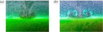
Long-exposure photographs of a vortex ring impinging on a sharp interface between an upper tracer-particle-laden fresh-water layer and a lower green-dyed salt-water layer. Photographs display a vortex ring (a) just prior to and (b) during the vortex-ring interaction. Here
 $\mathit{Ri}\gg 1$
.

In this study, we focus on the vortex-ring interaction with a two-layer stratification with a sharp interface. Figure 1 provides photographs of such an interaction. In these images, the more dense lower layer has been dyed green to highlight the density variation. The images clearly demonstrate the entrainment of the dense lower-layer fluid into the upper layer as a result of the vortex-ring interaction. While similar studies have focused on the mixing induced by a small number of vortex-ring events (Linden Reference Linden1973; Dahm, Scheil & Tryggvason Reference Dahm, Scheil and Tryggvason1989), here we discuss the mixing observed in the limit of a large number of vortex-ring events. Our results demonstrate a difference from the previous theory. Linden (Reference Linden1973) proposed that, for a vortex ring of diameter
 $a$
and propagation speed
 $U$
in a salt-stratified fluid, the entrainment velocity
 $u_{e}$
is related to the bulk Richardson number (
 $\mathit{Ri}$
) via the relationship
 $$\begin{eqnarray}\frac{u_{e}}{U}\propto \mathit{Ri}^{-3/2},\quad \text{where }\mathit{Ri}=g\frac{{\it\rho}_{2}-{\it\rho}_{1}}{{\it\rho}_{1}}\frac{a}{U^{2}}.\end{eqnarray}$$
Here,
 $g$
is the acceleration due to gravity, with densities of the homogeneous upper (
 ${\it\rho}_{1}$
) and lower (
 ${\it\rho}_{2}$
) layers. This theory was compared to the results of Turner’s mixing box experiment (Turner Reference Turner1968), the measurements of which were somewhat ambiguous as to whether the entrainment velocity scales as
 $\mathit{Ri}^{-1}$
or
 $\mathit{Ri}^{-3/2}$
. In contrast to the vortex-ring idealization of Linden’s theory, the experimental work of Moore & Long (Reference Moore and Long1971) for shear-induced mixing across a sharp interface suggested an
 $\mathit{Ri}^{-1}$
scaling for the entrainment velocity of a turbulent shear flow. A more recent investigation by Oglethorpe, Caulfield & Woods (Reference Oglethorpe, Caulfield and Woods2013) demonstrated that an
 $\mathit{Ri}^{-1}$
regime also occurs in stratified Taylor–Couette flow. Of critical importance is the characterization of the entrainment velocity. In particular, in the following discussion, each vortex ring represents a discrete mixing event and provides a volume of entrained fluid, rather than an entrainment velocity per se. We return to this issue below.
In this paper, we demonstrate that, in the limit of a large number of vortex-ring interactions, the system evolves to an
 $\mathit{Ri}^{-1}$
regime, consistent with the fully turbulent mixing of Moore & Long (Reference Moore and Long1971), Park, Whitehead & Gnanadeskian (Reference Park, Whitehead and Gnanadeskian1994) and Oglethorpe et al. (Reference Oglethorpe, Caulfield and Woods2013). In reference to the work of Linden (Reference Linden1979), the mixing efficiency is proportional to the product of the entrainment velocity and the Richardson number. As such, an
 $\mathit{Ri}^{-1}$
scaling for the entrainment rate corresponds to a constant mixing efficiency. Here, we directly measure the mixing efficiency of independent vortex-ring interactions. Mixing efficiency measurements are complicated owing to the large number of variables that must be measured in the system. A number of experimentally (Prastowo et al.
Reference Prastowo, Griffiths, Hughes and Hogg2008, Reference Prastowo, Griffiths, Hughes and Hogg2009; Davies Wykes & Dalziel Reference Davies Wykes and Dalziel2014) and numerically (Peltier & Caulfield Reference Peltier and Caulfield2003; Scotti & White Reference Scotti and White2011; Gayen, Hughes & Griffiths Reference Gayen, Hughes and Griffiths2013) measured mixing efficiencies have been reported. However, these results are typically measurements for internally mixed problems (Turner Reference Turner1979), where the mixing mechanism is generated near the mixing location. External mixing, in contrast to internal mixing, is where the source of the turbulence driving the mixing is not local to the site of the mixing (Turner Reference Turner1979). We extend this body of work with the efficiency of external mixing produced by vortex rings.
The remainder of this paper is organized as follows. In § 2 we introduce the experimental set-up. We then develop, in § 3, a new model of external mixing in a finite box and show that the model agrees with the experimental results of the many vortex-ring interactions in § 4. Finally, in § 5, we offer our conclusions and provide avenues for future research.
2. Experimental methods
The experiments described here were performed by generating many neutrally buoyant vortex rings in the upper layer of a nominally two-layer salt-stratified fluid with a sharp density interface. The vortex rings were directed vertically downwards into the more dense bottom layer. The interaction of the vortex ring with the stratification produced mixing of the density field. We focus on the potential energy evolution in the limit of a large number of independent vortex-ring mixing events. These vortex rings are an example of an external mixing mechanism (Turner Reference Turner1979), as the vortical structures driving the mixing are produced external to the location of mixing.
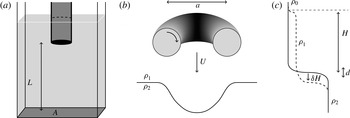
Sketch of (a) the tank set-up, (b) the physical parameters associated with the vortex ring and (c) the relevant parameters associated with the stratification.

The method of vortex-ring generation was similar to the work of Munro, Bethke & Dalziel (Reference Munro, Bethke and Dalziel2009) with the servo-motor used previously replaced by a linear actuator to allow automated generation of sequences of rings. A 3.9 cm hollow cylinder (tube) was inserted into the fluid and connected to a bicycle pump (2.9 cm internal diameter) driven by the linear actuator. Figure 2(a) sketches the tank set-up, where the tube is inserted into the centre of the tank, far from the tank walls and normal to the base of the tank. The tube is submerged so that the base is 18 cm below the water surface and
 $L\approx 30~\text{cm}$
above the maximum extension of the conductivity probe. By actuating the pump, the fluid within the tube was displaced downwards, resulting in the generation of a vortex ring at the base of the tube. Vortex rings are thus generated from fluid internal to the system, preserving the fluid volume. By digitally controlling the linear actuator, we are able to precisely control the propagation speed and timing of the generated vortex rings. The actuation length (
 ${\sim}15~\text{cm}$
, corresponding to a fluid displacement of 8.3 cm, provided the air is not compressed) and speed were varied in order to produce variations in the vortex-ring structure and speed to ensure consistency over a range of parameter values. Two different tank sizes (
 $0.2~\text{m}\times 0.4~\text{m}\times 0.5~\text{m}$
and
 $0.45~\text{m}\times 0.45~\text{m}\times 0.6~\text{m}$
) were used to ensure consistency of the results.
2.1. Velocity measurements
Using particle image velocimetry (PIV), we reconstruct the vorticity field within a thin vertical light sheet generated by masking the illumination from a pair of xenon arc lamps (300 W) with integrated paraboloidal dichroic reflectors producing
 ${\sim}35~\text{W}$
of visible light. The light sheet was aligned with the centre of the vortex generation tube. Using this method, we are able to reconstruct the planar flow field generated by individual vortex rings. DigiFlow (Dalziel Research Partners, Cambridge, UK) was used to perform the analysis of the particles. A similar approach was taken by Bethke & Dalziel (Reference Bethke and Dalziel2012). The video sequence was recorded with a Teledyne DALSA Falcon 2 (Teledyne DALSA Inc., Waterloo, Canada) camera (4 Mpixels), here with a frame rate of 150 f.p.s.
Both the vortex-ring diameter
 $a$
and propagating speed
 $U$
were determined via the computed vorticity field. The diameter was defined as the distance between the centroids of positive and negative vorticity. Similarly, the propagation speed was computed by tracking the vertical position of maximum vorticity in time. The average values were taken over multiple such computations. Errors are reported as the average difference between the individual case values and the average value. Figure 2(b) plots a diagram of the vortex-ring parameters.
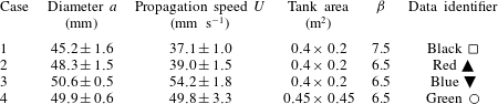
Table 1 presents the relevant parameters for the four different vortex-ring cases presented here. In the present work, the Reynolds number (
 $\mathit{Re}=Ua/{\it\nu}$
, for molecular viscosity
 ${\it\nu}$
) was varied only by 50 % (
 $\mathit{Re}=1700{-}2700$
). However, the change in vortex-ring propagation velocity allows us to vary the Richardson number independently of the stratification. We necessarily restrict our current discussion to vortex rings at moderate Reynolds numbers.
Table of the relevant characteristic parameters of the four different vortex-ring cases. Errors are reported as the average inter-generation difference in average diameter and propagation speed.

2.2. Density profiles
In order to determine the density change through successive vortex-ring generations, an aspirating conductivity probe (0.3 mm internal tip diameter) was used to measure density profiles through the tank. The conductivity of salt water is dependent on its salinity and temperature. By attaching a fast response thermistor (P25 NTC type, General Electric) to the conductivity probe, we measured both the conductivity and temperature of the water and, assuming no other solute in the fluid volume, we can back out the fluid density. This methodology is similar to that preformed in Davies Wykes & Dalziel (Reference Davies Wykes and Dalziel2014), and the reader is referred there for further information. The relative error in the point density measurements in this method has been shown to be
 $O(0.1\,\%)$
of the density range with which it has been calibrated. Other sources of signal noise in this system were compensated for by oversampling then filtering the data with both a median and spectral filter. Unlike the work of Davies Wykes & Dalziel (Reference Davies Wykes and Dalziel2014), we have attached a computer-controlled pinch valve to prevent fluid loss due to the aspiration while not measuring. In our experiments, the volume loss from aspiration can be shown to be
 $O(0.1\,\%)$
of the total volume in the tank.
The period between vortex rings was set to be
 ${\it\tau}\approx 75~\text{s}$
. Doubling this period yielded no quantitative difference, demonstrating that this period was sufficient for the motion to decay and for successive collisions to be independent. For most experiments, a single density profile measurement was taken every 10 vortex rings. The choice of sampling interval had no measurable influence on the evolution of the density field. Experiments were run for 600 vortex rings (resulting in 61 density profile measurements).
3. Theory
As we are interested in a sequence of temporally discrete mixing events, it is convenient to consider time as a discrete quantity. If we consider a sequence of
 $n$
vortex rings produced with a fixed inter-ring period
 ${\it\tau}$
, we can define discrete time
 $t_{n}=n{\it\tau}$
. The vortex-ring events will be independent (except through the resulting mixing of the density field) provided the time
 ${\it\tau}$
between successive vortex rings is such that the macroscopic motion within the fluid domain of interest has dissipated. We denote the time scale of this kinetic energy dissipation as
 ${\it\tau}_{\mathit{dissip}}$
. Thus, in order to ensure independence, we select
 ${\it\tau}>{\it\tau}_{\mathit{dissip}}$
.
On the other extreme, as we are interested in the change in potential energy due to each vortex ring, and not due to background diffusion, we restrict ourselves to the case where
 $$\begin{eqnarray}{\it\tau}_{\mathit{dissip}}<{\it\tau}\ll {\it\tau}_{\mathit{diffusion}}.\end{eqnarray}$$
Here,
 ${\it\tau}_{\mathit{diffusion}}=(1/{\it\kappa})(a^{3}/A)^{2}$
is the time scale of diffusion of the background density profile for molecular diffusivity
 ${\it\kappa}$
(
 ${\sim}1\times 10^{-9}~\text{m}^{2}~\text{s}^{-1}$
) over the vortex-ring equivalent-volume layer thickness
 $a^{3}/A$
for tank plan area
 $A$
. With reference to table 1, we see that, for case 4, the larger tank area decreases the diffusion time scale by a factor of four and the assumption of negligible background density diffusion begins to break down (
 ${\it\tau}\approx {\it\tau}_{\mathit{diffusion}}$
). This case has been included to ensure that the results presented here are robust.
Under these assumptions, the change in potential energy over each vortex-ring interaction (
 ${\rm\delta}$
PE) is produced by mixing the background density profile. The value of
 ${\rm\delta}$
PE was computed as the change in potential energy between conductivity probe measurements, divided by the inter-measurement number of vortex rings. The mixing efficiency is then defined as
 $$\begin{eqnarray}{\it\eta}=\frac{{\rm\delta}\text{PE}}{{\rm\delta}\text{KE}},\end{eqnarray}$$
for the initial kinetic energy of an individual vortex ring (
 ${\rm\delta}$
KE). In this paper, we will show that, under the conditions defined above and after an initial adjustment phase,
 ${\it\eta}$
is independent of
 $\mathit{Ri}$
and we recover the
 $\mathit{Ri}^{-1}$
scaling for the entrainment as discussed above.
3.1. Two-layer box model
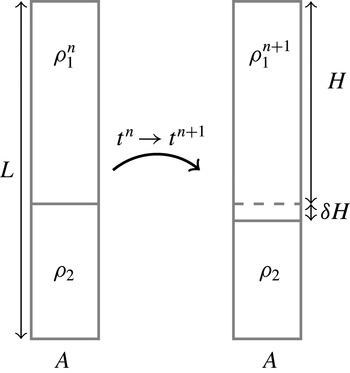
Consider a stably stratified finite-volume fluid in a box of height
 $L$
containing two homogeneous layers of densities
 ${\it\rho}_{1}$
and
 ${\it\rho}_{2}$
, divided by a sharp density interface. The height of the upper layer is
 $H$
, with the lower layer of height
 $L-H$
. Now, assume that the height of the density interface is lowered by a distance
 ${\rm\delta}H$
over a finite time
 ${\it\tau}=t_{n+1}-t_{n}$
. For the present discussion, we assume that both layers remain homogeneous over
 ${\it\tau}$
, with the lower layer remaining at a constant density. Uniformly mixed layers are typical of external mixing processes; see Turner (Reference Turner1968) and Oglethorpe et al. (Reference Oglethorpe, Caulfield and Woods2013). We will evaluate the effect of a non-homogeneously mixed upper layer later in this discussion. See figure 3 for a diagram of this two-layer box model.
Diagram of the change in density profiles between times
 $t_{n}$
and
 $t_{n+1}$
for the two-layer model.

The change in potential energy of this layered model (
 ${\rm\delta}\text{PE}_{L}$
) is
 $$\begin{eqnarray}{\rm\delta}\text{PE}_{L}=A\left(\int _{0}^{L}g{\it\rho}_{L}^{n+1}z\,\text{d}z-\int _{0}^{L}g{\it\rho}_{L}^{n}z\,\text{d}z\right).\end{eqnarray}$$
Assuming a homogeneously mixed upper layer, the density is given by
 $$\begin{eqnarray}{\it\rho}_{L}^{n}=\left\{\begin{array}{@{}ll@{}}{\it\rho}_{1}^{n}-\bar{{\it\rho}},\quad & z>L-H,\\ {\it\rho}_{2}-\bar{{\it\rho}},\quad & z<L-H,\end{array}\right.\quad {\it\rho}_{L}^{n+1}=\left\{\begin{array}{@{}ll@{}}{\it\rho}_{1}^{n+1}-\bar{{\it\rho}},\quad & z>L-H-{\rm\delta}H,\\ {\it\rho}_{2}-\bar{{\it\rho}},\quad & z<L-H-{\rm\delta}H.\end{array}\right.\end{eqnarray}$$
Here, and elsewhere in this paper, we remove the average density (
 $\bar{{\it\rho}}$
) from our computation of the change in potential energy. Mass conservation requires that the density of the upper layer will increase as
 $$\begin{eqnarray}\bar{{\it\rho}}=\frac{1}{L}\int _{0}^{L}{\it\rho}_{L}^{n+1}\,\text{d}z=\frac{1}{L}\int _{0}^{L}{\it\rho}_{L}^{n}\,\text{d}z,\quad {\it\rho}_{1}^{n+1}=\frac{{\it\rho}_{1}^{n}H+{\it\rho}_{2}{\rm\delta}H}{H+{\rm\delta}H}.\end{eqnarray}$$
Integrating through and retaining the leading-order term, assuming
 ${\rm\delta}H/H\ll 1$
, we find that
 $$\begin{eqnarray}\frac{{\rm\delta}\text{PE}_{L}}{AH}=\left[\frac{{\rm\delta}H}{a}\right]\left[\frac{1}{2}{\it\rho}_{1}U^{2}\right]\mathit{Ri},\end{eqnarray}$$
where
 $\mathit{Ri}$
is given by (1.1). The work of Linden (Reference Linden1973) can be modified to give an identical expression for the change in potential energy provided that we define the height of rise of the fluid after impact to be
 $H$
as opposed to
 $a$
and we write
 ${\rm\delta}H=\int _{{\it\tau}}u_{e}(t)\,\text{d}t$
.
As our experimental velocity measurements are on a single plane, they do not provide an independently rigorous estimate of the total kinetic energy of a single vortex ring (
 ${\rm\delta}$
KE), although they do provide a good measure of the propagation velocity and ring diameters. With reference to the theoretical results of Norbury (Reference Norbury1973),
 ${\rm\delta}$
KE is computed as
 $$\begin{eqnarray}{\rm\delta}\text{KE}={\it\beta}\left[\frac{1}{2}{\it\rho}_{0}U^{2}\right]\left[\frac{4}{3}{\rm\pi}\left(\frac{a}{2}\right)^{3}\right].\end{eqnarray}$$
The scaling coefficient
 ${\it\beta}$
is estimated through the theoretical prediction (for the relative core diameter of our rings) and verified by computing the kinetic energy of the vortex ring from our two-dimensional measurements assuming axisymmetry. We have determined
 ${\it\beta}\approx 6.5{-}7.5$
depending on the precise profiles; see table 1.
In our model, we are implicitly assuming that the effect of the diffusion of the background density profile is small and the effect of viscosity is negligible. Indeed, under the assumptions of this model, there are only two relevant dimensionless parameters,
 ${\it\eta}$
and
 ${\it\gamma}={\rm\delta}H/H$
. In a given experiment, if
 $H\gg {\rm\delta}H$
(i.e.
 ${\it\gamma}\ll 1$
), the mixing efficiency is constant and, where
 $H$
can be considered constant,
 ${\rm\delta}H$
(and hence the entrainment velocity,
 $u_{e}\approx {\rm\delta}H/{\it\tau}$
) scales as
 $\mathit{Ri}^{-1}$
. Indeed, we will show below that, after an initialization phase, these conditions hold in our experiment, and the mixing efficiency is indeed constant.
3.2. Density profile perturbation
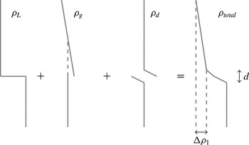
As will be discussed in § 4, the experimental density profiles deviate from the two-layer idealization utilized in the previous subsection. In particular, the experiments exhibit a weakly stable stratification in the upper layer and a finite interface thickness. In order to demonstrate the robustness of the results, we consider a simplified density profile that includes the contributions of an upper-layer gradient and a finite interface thickness, and compute the effect of these modifications on the potential energy change to the system. Figure 4 sketches, in an exaggerated manner, this decomposition of the simplified density profile (
 ${\it\rho}_{\mathit{total}}$
) into a two-layer profile
 $({\it\rho}_{L})$
as described previously, an upper-layer gradient perturbation (
 ${\it\rho}_{g}$
) and a finite interface thickness perturbation (
 ${\it\rho}_{d}$
). These profiles can be modelled as perturbations to the two-layer profile, written here as
 $$\begin{eqnarray}\displaystyle & {\it\rho}_{\mathit{total}}={\it\rho}_{L}+{\it\rho}_{g}+{\it\rho}_{d}, & \displaystyle\end{eqnarray}$$
 $$\begin{eqnarray}\displaystyle & {\it\rho}_{g}=\left\{\begin{array}{@{}ll@{}}\displaystyle \frac{{\rm\Delta}{\it\rho}_{1}^{n}}{H}\left(L-\frac{H}{2}-z\right),\quad & z\geqslant L-H,\\ 0,\quad & z<L-H,\end{array}\right. & \displaystyle\end{eqnarray}$$
 $$\begin{eqnarray}\displaystyle & {\it\rho}_{d}=\left\{\begin{array}{@{}ll@{}}0,\quad & z\geqslant L-H+d,\\ \displaystyle -\frac{{\rm\Delta}{\it\rho}}{2d}(z-(L-H+d)),\quad & L-H\leqslant z<L-H+d,\\ \displaystyle -\frac{{\rm\Delta}{\it\rho}}{2d}(z-(L-H-d)),\quad & L-H-d<z<L-H,\\ 0,\quad & z\leqslant L-H-d.\end{array}\right. & \displaystyle\end{eqnarray}$$
In this decomposition, we define the perturbations
 ${\it\rho}_{g}$
and
 ${\it\rho}_{d}$
to have net-zero mass. That is, both of these perturbations represent redistributions of the mass. These will change
 ${\rm\delta}$
PE as
 $$\begin{eqnarray}{\rm\delta}\text{PE}_{\mathit{total}}={\rm\delta}\text{PE}_{L}+{\rm\delta}\text{PE}_{g}+{\rm\delta}\text{PE}_{d}.\end{eqnarray}$$
The same subscript convention as for the density profiles is used here.
It is straightforward to show that, for a linear upper-layer stratification
 $\partial _{z}{\it\rho}_{1}={\rm\Delta}{\it\rho}_{1}/H$
, and a linear interface of thickness
 $d$
, the relative contributions of
 ${\rm\delta}$
PE are given by:
 $$\begin{eqnarray}\displaystyle \frac{{\rm\delta}\text{PE}_{g}}{{\rm\delta}\text{PE}_{L}} & = & \displaystyle -\frac{1}{6}\left[\frac{{\rm\Delta}{\it\rho}_{1}}{{\it\rho}_{2}-{\it\rho}_{1}}\right],\end{eqnarray}$$
 $$\begin{eqnarray}\displaystyle \frac{{\rm\delta}\text{PE}_{d}}{{\rm\delta}\text{PE}_{L}} & = & \displaystyle \frac{1}{12}\left[\left(\frac{d_{n+1}^{2}-d_{n}^{2}}{H{\rm\delta}H}\right)-\left(\frac{d_{n+1}^{2}}{H^{2}}\right)\right].\end{eqnarray}$$
 ${\rm\delta}$
PE
 $_{\mathit{total}}$
(i.e.
 ${\rm\delta}$
PE
 $_{\mathit{total}}<{\rm\delta}$
PE
 $_{L}$
).
Diagram of the decomposition of the simplified density profile (
 ${\it\rho}_{\mathit{total}}$
).

4. Results
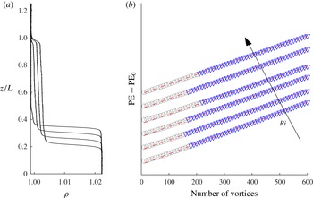
We now make a quantitative comparison between the two-layer model (3.6) and the experimental data. Figure 5(a) plots the density profiles of a single representative experiment after 10, 200, 400 and 600 vortex rings. These profiles demonstrate that there exists a mixing layer which develops above the density interface with some varying height
 $H$
. We denote this region as the middle mixed layer.
Plot of (a) the density profiles every 200 vortex rings and (b) the potential energy of each measured density profile. Six experiments are shown, with
 $\mathit{Ri}$
ranging between 4 (bottom curve) and 12 (top curve), increasing vertically. Note that a constant shift has been applied to the data in order to view the datasets individually. After an initial adjustment phase (grey circles), the change in potential energy becomes constant over the range of Richardson numbers.

We observe that the upward entrainment of each vortex ring is such that the interface moves downwards and the lower-layer density remains constant. We can envisage a process in which the fluid volume contained within the vortex ring, mixed with the entrained fluid, forms a new band at the bottom of the middle mixed layer as the kinetic energy of the ring is dissipated. This process will continue with each subsequent vortex ring, transporting a volume of fluid from the base of the vortex generation tube to the bottom of the middle mixed layer. This is analogous to the classical ‘filling box’ problem for a buoyant plume (Worster & Huppert Reference Worster and Huppert1983). Initially, the volume transport of the vortex rings will generate a middle mixed layer, which will increase in height with each subsequent vortex-ring interaction. We define the initial adjustment phase as the period before the top of the middle mixed layer reaches the base of the vortex tube. At the end of the initial adjustment phase, the initial vortex-ring density will be determined by the density at the top of the middle mixed layer and almost no further fresh water is injected into the system (ignoring the fluid displacement from the conductivity probe aspiration). This effectively isolates the fluid above the vortex generation point from the system. After the initial adjustment phase, just as in the two-layer model, the domain of interest
 $L$
(the sum of the lower-layer height and the middle-mixed-layer height) is constant. Subsequent vortex-ring generations continue the banding process, which results in the approximately linear stratification observed in the upper layer. The impact of this upper-layer stratification will be discussed below.
The evolution of the potential energy over all vortex-ring generations has been plotted (figure 5
b) for six representative experiments at different initial
 $\mathit{Ri}$
ranging from 4 to 12. The initial adjustment phase has been indicated by grey circles. After this adjustment period, all experiments demonstrate the same change in potential energy per vortex-ring mixing event, within experimental error, over the range of
 $\mathit{Ri}$
considered. That is,
 ${\rm\delta}$
PE is constant, in agreement with the dimensional analysis of the theoretical model. By varying the inter-vortex-ring spacing (
 ${\it\tau}$
), we estimate that an upper bound of 10 % of the potential energy increase is due to laminar diffusion of the background density stratification. However,
 ${\rm\delta}\text{PE}$
is not constant during the initial adjustment phase. This is due to a number of factors, including the variations in the initial density profile, and the rapidly growing middle mixed layer.
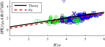
Figure 6 plots, for all experiments, the scaled
 ${\rm\delta}\text{PE}$
versus the normalized middle-mixed-layer height
 $H$
after the initial adjustment phase. As
 $H$
is determined as the height of the maximum density gradient of the density profile, small fluctuation in the profile may result in significant errors in the measurement of the middle-mixed-layer height. As there are a large number,
 $O(1000)$
, of density profiles measured, there exists a significant amount of noise in the plotted data. A five-point median filter was applied to each variable in order to smooth the data, and outliers were removed. The box-model equation (3.6) predicts a slope of
 $1/2$
and the least-squares linear fit through the data has a slope of
 $0.502\pm 0.038$
. As will be discussed below, contrary to our two-layer model, the upper-layer gradient and finite interface thickness are expected to cause the measured
 ${\rm\delta}$
PE to fall slightly below the model line, as observed. As noted in § 2, identifiers of the data presented here, and in subsequent figures, correspond to the cases presented in table 1. Note that, as the assumption of time scale separation between
 ${\it\tau}=75~\text{s}$
and
 ${\it\tau}_{\mathit{diffusion}}\approx 100~\text{s}$
is no longer strictly justified for the larger tank (circles), we do not include these points in the discussion of the density profile perturbations presented below.
Plot of the scaled
 ${\rm\delta}$
PE versus normalized
 $H$
. The theoretical curve is plotted in solid black and the fit to the data is displayed as a dashed line. Note that the fitted scale fits very well with the theoretical fit (0.502 versus
 $1/2$
).

4.1. Density profile perturbations
In the present work, the interface thickness
 $d$
is computed from the maximum density gradient
 $\partial _{z}{\it\rho}_{max}$
as
 $d=({\it\rho}_{2}-{\it\rho}_{1})/\partial _{z}{\it\rho}_{max}$
. This provides us with a relatively robust method of determining
 $d$
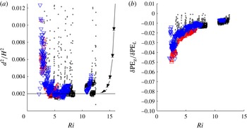
. Figure 7(a) plots
 $d^{2}/H^{2}$
versus
 $\mathit{Ri}$
, for comparison with the final term in (3.12b
). We observe that, regardless of the initial interface thickness, the vortex rings sharpen the interface and
 $d$
rapidly collapses to some function of the Richardson number. For large Richardson numbers, the interface thickness is constant (
 $d^{2}/H^{2}\approx 2\times 10^{-3}$
, hence the last term in (3.12b
) is dominant), consistent with the results of Shravat, Cenedese & Caulfield (Reference Shravat, Cenedese and Caulfield2012) for an entirely different external mixing mechanism. We expect the value of the constant interface thickness to depend on the other non-dimensional parameters of the problem. As the kinetic energy becomes dominant (low Richardson number), the vortex rings penetrate deeper into the lower layer and the vortex rings are no longer able to maintain an interface that is sharp.
(a) Plot of
 $d^{2}/H^{2}$
versus
 $\mathit{Ri}$
. Note that, for large Richardson numbers, this quotient tends to a constant. A constant line was plotted for comparison with a value of
 $2\times 10^{-3}$
. Diagrammatic arrows have been plotted depicting the time evolution of the interface thickness. (b) Plot of
 ${\rm\delta}\text{PE}_{g}/{\rm\delta}\text{PE}_{L}$
versus
 $\mathit{Ri}$
. Data points within the initial adjustment phase have been shaded grey.

Figure 7(b) plots
 ${\rm\delta}\text{PE}_{g}/{\rm\delta}\text{PE}_{L}$
versus
 $\mathit{Ri}$
to demonstrate the role played by the middle mixed layer. The middle-mixed-layer density difference
 ${\rm\Delta}{\it\rho}_{1}$
was computed using the average gradient within the middle mixed layer. As before, the data rapidly converge onto a single function of
 $\mathit{Ri}$
. This figure demonstrates that, for large
 $\mathit{Ri}$
, the relative change in the potential energy as a result of the middle-mixed-layer gradient is small and increases in magnitude with decreasing
 $\mathit{Ri}$
.
These results support the notion, through (3.12a,b
) that the variation in mixing rate as a result of the upper-layer gradient and finite interface thickness are small compared with the mixing rate observed for the two-layer evolution at large
 $\mathit{Ri}$
. As
 $\mathit{Ri}\rightarrow 0$
, the assumptions made in the two-layer model begin to break down and the impact of the density perturbations will increase. Thus, we argue that the mixing efficiency decreases as
 $\mathit{Ri}\rightarrow 0$
.
4.2. Mixing rate
It is clear that the dynamics of the initial adjustment phase are different from the constant-mixing-rate regime. As such, we introduce a transition Richardson number
 $\mathit{Ri}_{T}$
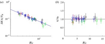
, defined as the bulk Richardson number determined at the end of the initial adjustment phase. Figure 8(a) plots
 ${\rm\delta}H$
normalized by the vortex-ring volume (
 $V_{R}$
) equivalent layer height after the initial adjustment phase versus
 $\mathit{Ri}_{T}$
. This is plotted for all four cases obtained in table 1, three in one tank and the additional case of a tank with a larger plan area (circles). An
 $\mathit{Ri}^{-1}$
fit (solid line) is provided for comparison. A least-squares fit of the data produces the relationship
 $$\begin{eqnarray}\frac{{\rm\delta}HA}{V_{R}}=0.695\mathit{Ri}^{-0.95\pm 0.13}.\end{eqnarray}$$
Here,
 $V_{R}=(4/3){\rm\pi}(a/2)^{3}$
is the approximate vortex-ring volume, only affecting the constant of proportionality. This power-law scaling is indistinguishable from the predicted
 $\mathit{Ri}^{-1}$
, once the error bars of the measurements are taken into account. From (3.6), we expect the change in interface position (
 ${\rm\delta}H$
) to differ slightly from the
 $\mathit{Ri}^{-1}$
relationship during the initial adjustment phase, as
 $H$
is also varying in time.
(a) Plot of the normalized
 ${\rm\delta}H$
as a function of
 $\mathit{Ri}_{T}$
. An
 $\mathit{Ri}^{-1}$
line was plotted for comparison. (b) Plot of the normalized mixing efficiency as a function of
 $\mathit{Ri}_{T}$
. Note that, as
 $\mathit{Ri}_{T}\rightarrow 0$
, we expect that
 ${\it\eta}$
will also tend to zero.

Using the Norbury scaling (3.7), figure 8(b) plots the mixing efficiency
 ${\it\eta}$
normalized by a constant reference
 ${\it\eta}_{0}$
as a function of
 $\mathit{Ri}_{T}$
. We see clearly that the mixing efficiency is constant over a range of vortex-ring parameters and
 $\mathit{Ri}$
. Since
 ${\rm\delta}$
KE is constant during an experiment, and experimental observations confirm that all of the vortex rings of a given experiment are of the same parameter set, our use of the Norbury theory to estimate
 ${\rm\delta}$
KE does not affect our conclusion that
 ${\it\eta}$
is constant. The method of estimating
 ${\rm\delta}$
KE does, however, affect the value of
 ${\it\eta}_{0}$
. In particular, using this approach, we estimate
 ${\it\eta}_{0}=4.2\times 10^{-1}$
. This value of the mixing efficiency is nearly double that of Linden (Reference Linden1979). The principle error in determining
 ${\it\eta}_{0}$
is in the estimate of the kinetic energy, but the precise value of
 ${\it\eta}_{0}$
does not alter the conclusion of a constant mixing efficiency. Future work will confirm the precise value of
 ${\it\eta}_{0}$
. As mentioned previously, at low
 $\mathit{Ri}$
, we expect that the mixing rate will decrease to zero.
5. Conclusion
By periodically generating temporally independent vortex rings which interact with a sharp interface, we externally mix the density stratification. The initial vortex rings evolve the stratification such that the density interface sharpens and a mixed fluid layer is generated above the density interface. This initial adjustment phase continues until the top of the mixed layer reaches the base of the vortex tube. After the initial adjustment phase, the system evolves such that the change in interface position is proportional to
 $\mathit{Ri}^{-1}$
.
In this work, we have a clear indication that this externally mixed system will evolve such that the mixing efficiency becomes independent of
 $\mathit{Ri}$
provided the following conditions hold. First,
 $\mathit{Ri}$
must be large enough that the interface thickness and upper-layer gradient remain small. Second, the system must be volumetrically constricted, in some sense, to restrict the height of the mixing layer
 $H$
. Third, the entrainment rate is sufficiently high that the molecular diffusion is not dominant and that the density interface remains sharp. Note that this regime is only attainable provided that the time scale of diffusion is long enough (low molecular diffusivity) such that the increase in potential energy is dominated by the mixing induced by the vortex rings. In the present experiments this is ensured by restricting the temporal inter-vortex-ring spacing, but it is our contention that this could have been equivalently performed by producing two spatially isolated vortex-ring events with a longer time interval between subsequent vortex rings. These may appear to be very limiting constraints to the problem; however Oglethorpe et al. (Reference Oglethorpe, Caulfield and Woods2013) observe the identical set-up and conclusion in a stratified Taylor–Couette flow. This mixing was driven by an entirely different mechanism of external mixing of the fluid (Taylor instability). Similarly, Moore & Long (Reference Moore and Long1971) observed an
 $\mathit{Ri}^{-1}$
entrainment relationship in a stratified shear flow. Again, Park et al. (Reference Park, Whitehead and Gnanadeskian1994) identified a similar layering mechanism with a constant mixing efficiency when considering a horizontally moving vertical rod. The results presented in this paper are consistent with observations made for a range of external mixing mechanisms. Future work will investigate the limits of applicability of this model including a variation of the Reynolds number and larger Richardson numbers.
While other studies of internal mixing problems have reported mixing efficiency values higher than those reported here (see Davies Wykes & Dalziel Reference Davies Wykes and Dalziel2014), the present value of
 ${\it\eta}_{0}$
is significantly higher than that reported for most other external mixing problems (see Linden Reference Linden1979). The largest source of uncertainty in these estimates is in the precise value of the kinetic energy through the parameter
 ${\it\beta}$
. It should be stressed again that our rings are highly reproducible and this error is in the quantification of the kinetic energy and not a random variation between experiments. We have estimated
 ${\it\beta}$
in four ways: (i) directly from our PIV data under the assumption of axisymmetry; (ii) using the PIV data but projecting the flow outside the cores onto an irrotational field to minimize the influence of spurious noise at large radius; (iii) the energy imparted to the fluid as it is displaced from the vortex tube; and (iv) following Norbury’s (Reference Norbury1973) analysis using an estimate of the dimensionless core size. These four measures produce broadly consistent results, with differences of less than 20 %. Although the cores do not have the constant
 ${\it\omega}/r$
assumed by Norbury, we have elected to adopt the Norbury approximation throughout for simplicity and consistency. While this choice of quantification for the kinetic energy impacts the precise value of
 ${\it\eta}_{0}$
, this does not alter our conclusion that the mixing efficiency
 ${\it\eta}$
is independent of
 $\mathit{Ri}$
. Clearly, more work is required to improve the precision of the
 ${\it\eta}_{0}$
estimate and understand the dynamics that allow it to be so high.
We briefly return here to the distinction between the entrainment rate
 $u_{e}$
and the discrete change in interface height
 ${\rm\delta}H$
. In this present work, the time scale of mixing has been removed from the problem. If we write
 $u_{e}\approx {\rm\delta}H/{\it\tau}_{M}$
for some time scale
 ${\it\tau}_{M}$
, then that choice of mixing scale affects the model for entrainment velocity (though not necessarily the mixing efficiency). In particular, if
 ${\it\tau}_{M}$
is proportional to linear long-wave period, and so a function of
 $\mathit{Ri}$
rather than the fixed value of
 ${\it\tau}$
we have used, then we see that the theory of Linden (Reference Linden1973) is a special case of the work done here. This present work quantifies the increase in potential energy of the system for a given kinetic energy input (mixing efficiency). Future work will examine the time scales associated with different external mixing problems.
While these results demonstrate an important feature of periodic externally forced stratified mixing, there remain many unanswered questions. For example, the balance leading to a fixed interface thickness
 $d$
and weak upper-layer gradient need to be determined as well as gaining a better understanding of the initial adjustment phase.
Acknowledgements
This work was funded through the support of the Natural Sciences and Engineering Research Council of Canada (NSERC) and the Engineering and Physical Sciences Research Council (EPSRC) grant number EP/L504920/1. The experimental data associated with this study are made available at https://www.repository.cam.ac.uk/handle/1810/249285.