
1. Introduction
Settling of relatively small, inertial particles in turbulence is of importance in numerous geophysical, biological and engineering applications such as sediment transport (Finn, Li & Apte Reference Finn, Li and Apte2016; Dey et al. Reference Dey, Ali and Padhi2019, Reference Dey, Ali and Padhi2020; Vowinckel Reference Vowinckel2021; Li, Bragg & Katul Reference Li, Bragg and Katul2023), plankton dynamics (Bergkvist et al. Reference Bergkvist, Klawonn, Whitehouse, Lavik, Brüchert and Ploug2018) and aerosol distribution in the atmosphere (Maxey Reference Maxey1987). Prediction of these very large-scale natural processes commonly employs models that heavily rely on accurate estimation of the average particle settling speed in a turbulent flow. Terminal settling speeds of particles depend on the shape, size and density of particles, concentration or volume loading and characteristics of turbulence. In still fluid, the settling speed is determined through a force balance between the net weight and hydrodynamic forces exerted by the fluid. However, when settling through turbulence, the presence of rapidly evolving eddies, characterised by a broad range of length and time scales, significantly complicates this dynamics (Dey, Ali & Padhi Reference Dey, Ali and Padhi2019). Furthermore, different particle properties such as the particle size relative to these eddies and particle density compared with the fluid can have a significant effect on the resulting dynamics due to two-way interactions between the fluid and particles (Nielsen Reference Nielsen1993, Reference Nielsen2007; Kawanisi & Shiozaki Reference Kawanisi and Shiozaki2008; Jacobs et al. Reference Jacobs, Merchant, Jendrassak, Limpasuvan, Gurka and Hackett2016).
At very high volume loading, particle collisions result in hindered settling (Richardson & Zaki Reference Richardson and Zaki1954). At low-to-moderate volume loading, turbulence can lead to enhancement or retardation of terminal speeds through four key mechanisms (Nielsen Reference Nielsen1993; Dey, Ali & Padhi Reference Dey, Ali and Padhi2020): (i) vortex trapping, (ii) fast tracking, (iii) loitering and (iv) nonlinear drag. Vortices can trap small and slightly heavier particles, reducing their fall velocity, whereas very heavy particles get thrown out of vortices due to centrifugal forces. Temporal variations in vortex strength can affect this ‘vortex trapping’ phenomenon. Heavier-than-fluid inertial particles tend to accumulate in low vorticity regions of the flow, where the fluid velocity aligns with the direction of gravity, and follow the path of least resistance. This is known as ‘fast tracking’ or ‘preferential sweeping’ and tends to increase the settling speed. Whereas, when particles are too swift to be directed along the fast track or if the vortices are short lived, then the particles spend more time in the region where the fluid flows in the opposite direction, causing them to ‘loiter’ in these regions, reducing the settling speed. Finally, as the particle Reynolds number becomes large, the nonlinear inertial and unsteady effects on the drag forces become important, affecting the settling speeds. Fast tracking increases the settling speed, whereas vortex trapping, nonlinear drag and loitering tend to decrease it. However, under what conditions turbulence leads to enhanced or retarded settling speeds is still not completely understood and even the existence of the effects of nonlinear drag and loitering mechanisms has been questioned (Good et al. Reference Good, Ireland, Bewley, Bodenschatz, Collins and Warhaft2014; Ireland & Desjardins Reference Ireland and Desjardins2017; Akutina et al. Reference Akutina, Revil-Baudard, Chauchat and Eiff2020).
Dávila & Hunt (Reference Dávila and Hunt2001) discuss three methods of averaging the settling speed in studying particles settling around a Rankine vortex: (i) an Eulerian average, that is the average of the particle settling speeds at a particular point weighted by the particles’ concentration distribution, (ii) a Lagrangian average wherein the average is taken over an ensemble of particles starting from different locations and (iii) a bulk average. The key variable of interest is the normalised settling speed of the particles,
 $\langle V_S \rangle / V_T^0$
, where
 $\langle V_S \rangle$
is the mean settling speed obtained in the present work by averaging each particle’s settling speed over time and then ensemble averaging over all particles,
 $V_T^0(=\tau _p g)$
is the terminal settling speed in quiescent fluid,
 $g$
is the magnitude of the gravitational acceleration and
 $\tau _p$
is the particle relaxation time. The normalised settling speed of spherical particles is a function of several non-dimensional parameters
 \begin{equation} \frac {\langle V_S \rangle }{V_T^0} = {\mathcal F}\left (St_{\eta }, Sv_{\eta }, Re_{\lambda }, \phi \right ), \end{equation}
where
 $St_{\eta }$
is the Stokes number,
 $Sv_{\eta }$
is the settling parameter,
 $Re_{\lambda }$
is the Taylor-microscale Reynolds number and
 $\phi$
is the volume loading of the particles. The Stokes number,
 $St_{\eta }$
, and settling parameter,
 $Sv_{\eta }$
, are defined as
 \begin{equation} St_{\eta } = \frac {\tau _p}{\tau _{\eta }} = \underbrace {\left (\frac {(R_{\rho }-1)}{18}\frac {d_p^2}{\nu }\right ) }_{\tau _p} \underbrace {\left (\frac {\epsilon ^{0.5}}{\nu ^{0.5}}\right ) }_{\tau _{\eta }^{-1}} = \left (\frac {R_{\rho }-1}{18}\right ) \left (\frac {d_p}{\eta }\right ) ^2, \end{equation}
and
 \begin{equation} Sv_{\eta } = \frac {St_{\eta }}{Fr} = \underbrace {\left (\frac {\tau _p}{\tau _{\eta }}\right ) }_{St_{\eta }} \underbrace {\left (\frac {g}{a_{\eta }}\right ) }_{Fr^{-1}} = \frac {V_T^0}{u_{\eta }}. \end{equation}
Here,
 $\epsilon$
is the dissipation rate,
 $\nu$
is the kinematic viscosity,
 $u_{\eta }$
,
 $a_{\eta }$
,
 $\tau _{\eta }$
and
 $\eta$
are the Kolmogorov velocity, acceleration, time and length scales,
 $u'$
is the turbulence intensity and
 $Fr$
is the Froude number. The particle-to-fluid density ratio (
 $R_{\rho }=\rho _p/\rho _f$
) and particle diameter to Kolmogorov length scale ratio (
 $d_p/\eta$
) are also important parameters and appear indirectly in the Stokes number and settling parameter. The settling parameter can be similarly expressed in terms of the turbulence intensity
 \begin{equation} Sv_{\ell } = \frac {V_T^0}{u'} = Sv_{\eta }Re_{\lambda }^{-1/4}, \end{equation}
where
 $Re_{\lambda } = u'\lambda /\nu$
is the Reynolds number associated with the Taylor microscale,
 $\lambda$
. In this study, we are interested in the inverse of this quantity,
 $Sv_{\ell }^{-1} = u'/V_T^0$
, which will also be referred to as the normalised turbulence intensity.
Strong preferential concentration and clustering of small, inertial particles happens when the particle relaxation time and Kolmogorov time scales match for
 $St_{\eta }\sim 1$
(Eaton & Fessler Reference Eaton and Fessler1994). For very heavy particles,
 $R_{\rho }\sim {\mathcal O}(1000)$
, this is achieved when the particle size is small compared with the Kolmogorov scale (
 $d_p \lesssim 0.13\eta$
) from (1.2). For the dynamics of these small, heavy particles, the drag and gravity forces are most dominant. Extensive experimental (Good et al. Reference Good, Ireland, Bewley, Bodenschatz, Collins and Warhaft2014; Nemes et al. Reference Nemes, Dasari, Hong, Guala and Coletti2017; Petersen, Baker & Coletti Reference Petersen, Baker and Coletti2019) and computational work (Maxey Reference Maxey1987; Wang & Maxey Reference Wang and Maxey1993; Bosse, Kleiser & Meiburg Reference Bosse, Kleiser and Meiburg2006; Bec, Homann & Ray Reference Bec, Homann and Ray2014; Ireland, Bragg & Collins Reference Ireland, Bragg and Collins2016; Rosa et al. Reference Rosa, Parishani, Ayala and Wang2016; Monchaux & Dejoan Reference Monchaux and Dejoan2017; Tom & Bragg Reference Tom and Bragg2019; Rosa, Pozorski & Wang Reference Rosa, Pozorski and Wang2020; Tom, Carbone & Bragg Reference Tom, Carbone and Bragg2022) conducted in this regime predominantly observed the fast tracking mechanism for increased settling speeds, however, retardation due to loitering or vortex trapping was absent. Good et al. (Reference Good, Ireland, Bewley, Bodenschatz, Collins and Warhaft2014) did observe settling speed reduction in experiments, but were only able to reproduce this reduction due to the loitering mechanism in simulations by employing nonlinear drag or by using linear drag and artificially restricting particles to vertical paths.
For slightly heavier-than-fluid particles,
 $R_{\rho }\sim {\mathcal O}(10)$
, to get
 $St_{\eta }\sim 1$
, particle sizes should be comparable to the Kolmogorov scale (
 $d_p\sim \eta$
). These conditions correspond to sand particles in water (
 $R_{\rho }\sim 2.6$
) in coastal regions or river/streams with oscillatory or steady boundary layers (Foster, Beach & Holman Reference Foster, Beach and Holman2006; Cuthbertson & Ervine Reference Cuthbertson and Ervine2007; Finn et al. Reference Finn, Li and Apte2016; Hagan et al. Reference Hagan, Wengrove, Dubief, Desjardins, Frank-Gilchrist and Calantoni2023). For this regime, Nielsen (Reference Nielsen2007) assembled experimental data on the mean settling speed as a function of the normalised turbulence intensity (figure 1). If turbulence is weak (
 $Sv_{\ell }^{-1}\lesssim 0.4)$
, the settling speed is unaffected as compared with quiescent fluid. For very strong turbulence (
 $Sv_{\ell }^{-1}\gtrsim 4)$
, enhanced settling is observed. For moderate turbulence (
 $0.4 \lesssim Sv_{\ell }^{-1} \lesssim 4$
), experimental data (Murray Reference Murray1970; Kawanisi & Shiozaki Reference Kawanisi and Shiozaki2008) show reduced settling speeds and this is attributed to particles oversampling upward moving fluid, i.e. the loitering effect. However, a few experimental studies (Yang & Shy Reference Yang and Shy2003; Jacobs et al. Reference Jacobs, Merchant, Jendrassak, Limpasuvan, Gurka and Hackett2016) also found enhanced settling suggesting presence of fast tracking. If particle sizes are much larger than the Kolmogorov scale (
 $d_p/\eta \gt 10$
), experimental data (Akutina et al. Reference Akutina, Revil-Baudard, Chauchat and Eiff2020) and particle resolved direct simulations (Fornari et al. Reference Fornari, Picano, Sardina and Brandt2016) showed a decrease in the settling speeds, suggesting that the particle size may also play an important role in this regime. This reduction in settling speed increases for increasing turbulence intensity relative to the terminal speed in quiescent fluid and is suspected to be due to loitering, nonlinear drag or some combination of the two.
Normalised settling speed as a function of the normalised turbulence intensity.

Finally, the volume loading,
 $\phi$
, can also have a significant effect on the group settling dynamics. With larger volume loading (
 $\phi \gtrsim \ \textit {O}(10^{-3})$
), particle-to-particle interactions become important and affect the particle dynamics through hindered settling and clustering. For such volume loadings, particle–particle collisions should be accounted for (Kuerten Reference Kuerten2016; Rosa et al. Reference Rosa, Pozorski and Wang2020; Dey et al. Reference Dey, Ali and Padhi2020). In very dilute systems (
 $\phi \lesssim \ \textit {O}(10^{-6})$
) the particles do not meaningfully impact the carrier fluid. Recent works (Monchaux & Dejoan Reference Monchaux and Dejoan2017; Tom et al. Reference Tom, Carbone and Bragg2022; Bhattacharjee et al. Reference Bhattacharjee, Tom, Carbone and Bragg2024) showed that, in this very dilute regime, particles do not affect the global fluid statistics, such as the total turbulent kinetic energy, but may locally disturb the fluid in a way which modifies the particle settling speed. These studies focused on small, heavy particles and showed enhanced settling speeds. Monchaux & Dejoan (Reference Monchaux and Dejoan2017) attribute the enhanced settling rates of these types of particles to a two-way-coupled fluid dragging effect, where particles locally pull the fluid with them, reducing their slip velocity and thus reducing drag forces, rather than fast tracking. Tom et al. (Reference Tom, Carbone and Bragg2022) used multiscale analysis to identify that, while this fluid dragging effect is present, the main factor leading to enhanced settling rates is still fast tracking, just at different flow scales.
It is clear that slightly heavier-than-fluid particles of size of the order of the Kolmogorov scale have not been studied in detail. The present study focuses on this regime in moderate volume loading. The first goal of this study is to quantify how homogeneous, isotropic turbulence modifies the settling rates of sediment-like, Kolmogorov-scale, slightly heavier-than-fluid particles. As the first step, the Stokes number and turbulence intensity relative to the particle terminal settling speed in quiescent fluid are varied, whereas the volume loading is kept constant at moderate level (
 $\phi =10^{-3}$
). In the limit of weak turbulence, the particle group settling speed should approach that in the quiescent fluid. However, as the turbulence intensity is increased, the particles are carried by the turbulence structures or they resist the turbulent motion. The main objective is to investigate under what conditions fast tracking enhances settling speed and loitering or vortex trapping decreases settling speed for the specific parameter range of slightly heavier-than-fluid, Kolmogorov-scale particles.
The second goal is to identify which scales of turbulence directly influence the settling dynamics of these particles. To this end, the angular multiscale analysis of trajectory curvature angles (Kadoch et al. Reference Kadoch, Bassenne, Esmaily-Moghadam, Schneider, Farge and Bose2016; Apte et al. Reference Apte, Oujia, Matsuda, Kadoch, He and Schneider2022) is used by comparing the trajectory curvature angle statistics of particles with that of fluid tracers to discern which time scales of turbulence structure affect the particle dynamics. In addition, to identify the turbulence length scales that influence the vortex trapping versus fast tracking of particles, a multiscale wavelet analysis is performed on the fluid velocity seen by the particle and the second invariant of the velocity gradient tensor (Johnson & Wilczek Reference Johnson and Wilczek2024),
 $\mathcal{Q} = -A_{ik}A_{ik}/2 = \omega _i \omega _i/4 - S_{ij}S_{ij}/2$
, where
 $\unicode{x1D63C}$
is the velocity gradient tensor,
 $\boldsymbol{\omega }$
is vorticity and
 $\unicode{x1D64E}$
is the strain-rate tensor. By examining the values of
 $\mathcal{Q}$
sampled by inertial particles,
 $\mathcal{Q}^p(t)=\mathcal{Q}(\boldsymbol{x}_p(t),t)$
, one can identify whether the particles are preferentially sampling the flow and, if so, whether it is in strain-rate dominated (
 $\mathcal{Q}^p(t)\lt 0$
) or vorticity dominated (
 $\mathcal{Q}^p(t)\gt 0$
) regions, which can then be linked to fast tracking or vortex trapping mechanisms, respectively. The fluid velocity seen by the particles also helps identify the scales of turbulence affected by the particles.
To accurately capture the particle dynamics of Kolmogorov-scale, slightly heavier-than-fluid particles, the particle resolved approaches become unreasonably expensive as they require extreme resolutions, much finer than the Kolmogorov scales and hence are rare (Schneiders, Meinke & Schröder Reference Schneiders, Meinke and Schröder2017; Mehrabadi et al. Reference Mehrabadi, Horwitz, Subramaniam and Mani2018). Use of the point-particle approach is computationally viable; however, it also requires addressing several challenges. Firstly, the entire Maxey–Riley–Gatignol (MRG) equation of motion (Maxey & Riley Reference Maxey and Riley1983; Gatignol Reference Gatignol1983) must be considered, including the computationally expensive Basset history force (Ling, Parmar & Balachandar Reference Ling, Parmar and Balachandar2013; Olivieri et al. Reference Olivieri, Picano, Sardina, Iudicone and Brandt2014; van Hinsberg, Clercx & Toschi Reference van Hinsberg, Clercx and Toschi2017; Jaganathan et al. Reference Jaganathan, Prasath, Govindarajan and Vasan2023). Efficient and accurate methods of approximating this force have been developed (Moreno-Casas & Bombardelli Reference Moreno-Casas and Bombardelli2016) and the method of van Hinsberg, ten Thije Boonkkamp & Clercx (Reference van Hinsberg, ten Thije Boonkkamp and Clercx2011) is used. Secondly, for finite-sized, Kolmogorov-scale particles, even though the volume loading is moderate (
 $\phi \sim 10^{-3}$
), the low density ratio results in small mass loading, thus the particles do not have significant global impact on the fluid. However, as particles are large, and roughly 1–3 times larger than the grid resolution for the direct numerical simulation (DNS) of isotropic turbulence, they can significantly modify the local flow field, and hence the use of two-way coupling is necessary. Thirdly, the main assumption of the point-particle approach, which allows modelling of the particles as subgrid point sources, is no longer valid. This poses a problem when calculating particle forces using typical force closures that are defined based on particle slip velocity, which requires the undisturbed fluid velocity seen by that particle. That is, a fluid velocity field that does not include the self-disturbance created by the particle. Such a flow field is not readily available as particles locally disturb the fluid. A majority of the previous studies investigating small, heavy particles using a two-way-coupled, point-particle approach (Monchaux & Dejoan Reference Monchaux and Dejoan2017; Tom et al. Reference Tom, Carbone and Bragg2022; Bhattacharjee et al. Reference Bhattacharjee, Tom, Carbone and Bragg2024) used the disturbed fluid velocity in the force closures with the assumption that particle self-disturbance is small. However, when particles are finite sized, this approximation can lead to significant errors in particle and fluid statistics (Keane et al. Reference Keane, Apte, Jain and Khanwale2023). Correction schemes which aim to recover an estimate of the undisturbed fluid velocity have been developed, including a recent method used here wherein the particle self-disturbance field is obtained by solving an advection-diffusion-reaction equation in a small region surrounding each particle (Pakseresht & Apte Reference Pakseresht and Apte2021; Apte Reference Apte2022; Keane et al. Reference Keane, Apte, Jain and Khanwale2023).
The above point-particle model has been thoroughly validated against the particle-resolved simulations of decaying isotropic turbulence (Mehrabadi et al. Reference Mehrabadi, Horwitz, Subramaniam and Mani2018) of heavy, Kolmogorov-scale particles to verify that the particle–turbulence interactions, and influence of Kolmogorov-scale particles on the turbulent kinetic energy and dissipation rates, are accurately captured (Keane et al. Reference Keane, Apte, Jain and Khanwale2023). Some results from this validation can be found in Appendix A. The verified model and the multiscale analysis techniques are first applied to an idealised case of particles settling in a steady Taylor–Green vortex array wherein the vortex strength (intensity) is varied in relation to the particle settling speed. Owing to the steady nature of the flow, it is straightforward to visualise and analyse the fast tracking, loitering and vortex trapping mechanisms in this case. Then, the study of particle–turbulence interactions in a homogeneous, isotropic turbulence are performed for three different Stokes numbers and five different settling parameters.
The rest of the paper is arranged in the following way. Section 2 provides the details of the point-particle model, set-up of the idealised Taylor–Green vortex array case study as well as details of the DNS set-up and parameters for the homogeneous isotropic turbulence cases. In § 3, the results of slightly heavier-than-fluid particles settling in an idealised Taylor–Green vortex array followed by the parametric study of Kolmogorov-scale particles settling through homogeneous isotropic turbulence are described. Various statistics used to identify mechanisms in which the turbulence is modifying sediment settling rates are discussed in addition to wavelet-based multiscale analysis of preferential sampling in the homogeneous, isotropic turbulence cases. Finally, summary and conclusions are given in § 4.
2. Methods
The formulation of this model is based on the incompressible Navier–Stokes equations
 \begin{align} &\qquad\qquad\qquad\qquad\qquad\qquad \frac {\partial {u_i}}{\partial {x_i}} = 0, \end{align}
 \begin{align}& {\rho _f}\left (\frac {\partial {u_i}}{\partial {t}} + \frac {\partial {u_j u_i}}{\partial {x_j}} \right )= -\frac {\partial {p}}{\partial {x_i}} + {\mu }\frac {\partial ^2 {u_i}}{\partial {x_j}^2} + \underbrace {\left (-\sum _{q=1}^{N_p} {\mathcal G}^{\sigma }(\boldsymbol{x}_{cv}-\boldsymbol{x}_{q})F^t_{i,q}\right )}_{{\dot S_i}}, \end{align}
where
 $\rho _f$
is the density of the fluid,
 $\mu$
is the dynamic viscosity,
 $p$
is the pressure and
 ${u}_i$
is the two-way-coupled fluid velocity that includes the disturbances created by all
 $N_p$
particles through the net interphase source term (
 $\dot S_i$
). This interphase source term is based on all forces (
 $F_{i,q}^t$
), except gravity, acting on the particle located at
 ${\boldsymbol x}_q$
and projected onto the Eulerian grid control volumes located at
 ${\boldsymbol x}_{cv}$
, using the interpolation kernel
 ${\mathcal G}^{\sigma }$
, where
 $\sigma$
is the standard deviation of the kernel, thus representing kernel width. The projection function satisfies the conservation condition,
 $\int _{\mathcal V}{\mathcal G}^{\sigma }{\rm d}{\mathcal V} = 1$
, where the integration is over the whole fluid volume (
 $\mathcal V$
).
2.1. Point-particle model
Inertial particles are modelled following a point-particle approach, in which the Lagrangian equations for the motion of the
 $p^{\text{}}$
th particle are
 \begin{equation} \frac {{\rm d}x_{i,p}}{{\rm d}t} = u_{i,p},\ \ \ m_p\frac {{\rm d}u_{i,p}}{{\rm d}t} = m_p\left (1-\frac {\rho _f}{\rho _p}\right ) g_i + F_{i,p}^t \ , \end{equation}
where
 $x_{i,p}$
and
 $u_{i,p}$
are the particle position and velocity, respectively,
 $m_p$
is the mass of the particle and
 $F_{i,p}^t$
represents the forces acting on the particle including the drag, lift, added mass, pressure and Basset history force (Maxey Reference Maxey1987). These hydrodynamic forces are expressed as
 \begin{align}&\qquad\quad\,\, \boldsymbol{F}_d = m_p\frac {C_d}{\tau _p} \left (\boldsymbol{u}^{u,p}_{f|_p} - \boldsymbol{u}_{p}\right ), \end{align}
 \begin{align}& \boldsymbol{F}_l = m_p\frac {\rho _f}{\rho _p}C_l \left (\boldsymbol{u}^{u,p}_{f|_p} - \boldsymbol{u}_{p}\right ) \times \left ( \boldsymbol{\nabla } \times \boldsymbol{u}^{u,p}_{f|_p} \right ), \end{align}
 \begin{align}&\quad \boldsymbol{F}_{am} = m_pC_{am}\frac {\rho _f}{\rho _p} \left ( \frac {D\boldsymbol{u}^{u,p}_{f|_p}}{Dt} - \frac {{\rm d}\boldsymbol{u}_p}{{\rm d}t} \right ), \end{align}
 \begin{align}&\qquad\qquad\quad \boldsymbol{F}_{pr} = -\frac {m_p}{\rho _p} \boldsymbol{\nabla } P|_p, \end{align}
 \begin{align}&\, \boldsymbol{F}_h = \frac {3}{2}d_p^2\rho _f \sqrt {\pi \nu } \int _{-\infty }^t K_B(t-\tau )\boldsymbol{g}(\tau ){\rm d}\tau , \end{align}
where the Basset history force convolution function,
 $\boldsymbol{g}(t)$
, and its kernel are
 \begin{align} \boldsymbol{g}(t) = \frac {{\rm d}\boldsymbol{f}(t)}{{\rm d}t}, \quad \boldsymbol{f}(t) = \boldsymbol{u}^{u,p}_{f|_p} - \boldsymbol{u}_{p}, \quad K_B(t) = \frac {1}{\sqrt {t}}, \end{align}
and the chosen coefficients for drag, lift and added mass are
 \begin{align}&\qquad C_d = 1+0.15Re_p^{0.687}, \end{align}
 \begin{align}& C_l = \frac {1.61 \times 6}{\pi d_p} \sqrt {\frac {\mu }{\rho _f \left | \left ( \boldsymbol{\nabla } \times \boldsymbol{u}^{u,p}_{f|_p} \right ) \right |}}, \end{align}
 \begin{align}&\qquad\qquad\quad C_{am} = 0.5, \end{align}
where
 $\boldsymbol{u}^{u,p}_{f|_p}$
is the undisturbed fluid velocity seen by the particle
 $p$
and interpolated to the particle location,
 ${\boldsymbol x}_p$
. This undisturbed fluid velocity is obtained by removing the self-disturbance created by particle
 $p$
using the zonal-advection-diffusion-reaction (ADR) method (Apte Reference Apte2022; Keane et al. Reference Keane, Apte, Jain and Khanwale2023), discussed further below.
The drag force follows the Schiller and Naumann nonlinear correction for drag coefficient (2.10) based on the particle Reynolds number,
 $Re_p = \rho _f d_p |u^{u,p}_{i,f|_p} - u_{i,p}|/\mu$
. In the turbulent cases discussed in this paper, the particle Reynolds number remains in the
 $\textit {O}(1-10)$
range, thus the nonlinear drag model is used throughout the study. Only shear-based contributions to the lift force,
 $\boldsymbol{F}_l$
, are considered, and the lift coefficient (2.11) follows the closure of Saffman (Reference Saffman1965). Faxén corrections are included in the point-particle model to account for the finite size of the sediment-like particles, although at the particle sizes tested, this effect is minimal (Calzavarini et al. Reference Calzavarini, Volk, Bourgoin, Lévêque, Pinton and Toschi2009).
2.1.1. Basset history force
In the coastal sediment parameter regime studied here, the low density ratio and finite size of the particles results in the potential importance of every particle force in the equation of motion. The inclusion of the Basset history force (2.8) has historically been the most problematic due to the computational expense required to calculate it, as the full force requires each particles relative acceleration to be stored for the duration of the simulation in order to compute a time integral over the particles complete history at each time step. Often, this computational expense results in the neglect of the history force in point-particle simulations despite its potential relative importance (Ling et al. Reference Ling, Parmar and Balachandar2013; Moreno-Casas & Bombardelli Reference Moreno-Casas and Bombardelli2016; Jaganathan et al. Reference Jaganathan, Prasath, Govindarajan and Vasan2023).
In order to obtain the most realistic particle dynamics in this coastal sediment parameter regime, the Basset history force must be included. In order to address the issue of computational expense, Dorgan & Loth (Reference Dorgan and Loth2007) used a finite window over which the Basset history integral is evaluated. However, due to the standard kernel used for the Basset history force in (2.8), the decay is too slow to result in a convergent integral, thus requiring a large number of points to be included in the window period, greatly limiting performance. The other issue is that the history kernel is singular as
 $t \rightarrow 0$
. Moreno-Casas & Bombardelli (Reference Moreno-Casas and Bombardelli2016) review specific quadrature rules for the integral which resulted in nearly
 ${\mathcal O}(\Delta t)$
evaluation. Alternatively, Parmar et al. (Reference Parmar, Annamalai, Balachandar and Prosperetti2018) converted the integral into a differential form to make it easier to compute and to alleviate computational expense.
To address the slow decay of the kernel and singularity at
 $t=0$
, the novel numerical approach developed by van Hinsberg et al. (Reference van Hinsberg, ten Thije Boonkkamp and Clercx2011) is implemented. Due to the form of the history force kernel (2.9), the latest simulation time steps carry the most weight in the force calculation and van Hinsberg et al. (Reference van Hinsberg, ten Thije Boonkkamp and Clercx2011) found that the shape of the kernel for later times could be reasonably well captured with a sum of exponential functions. Thus, in this method, the Basset history force is decomposed into two portions, the ‘window’, which covers the most recent time history, and the ‘tail’, which is approximated by an exponential function. The history integral (2.8) is computed directly over the window period, which contains the three most recent time steps in the present model, and then the tail portion is modelled recursively using a linear combination of exponential functions which is simply added for each new time step. This approach limits the computational expense to storing the relative acceleration of each particle only over the window period rather than over the entire simulation. Casas, Ferrer & Oñate (Reference Casas, Ferrer and Oñate2018) further examined this method with a specific interest in optimising the free parameters that appear in each exponential function comprising the tail portion. These optimised free parameters are implemented in the present model. The contributions of these exponential functions are obtained in a recursive way, making the method computationally efficient. This approach decreased the computational time by more than an order of magnitude, but also resulted in
 ${\mathcal O}(\Delta t^2)$
approximation, consistent with the temporal accuracy of the numerical solver. In addition, a trapezoidal-based method is used to deal with the singularity at
 $t \rightarrow 0$
, which is also second-order accurate.
This method of calculating the history force has been tested in particle-laden homogeneous, isotropic turbulence previously (van Hinsberg et al. Reference van Hinsberg, Clercx and Toschi2017). It was identified as a good balance between computational efficiency and accuracy (Moreno-Casas & Bombardelli Reference Moreno-Casas and Bombardelli2016). A systematic evaluation of the above approach was conducted by varying the ‘window’ size and identifying its effect on the settling speed of a particle in quiescent fluid. It was observed that using only three previous history states in the direct integration and the rest obtained from the exponential match were sufficient to accurately capture the effect of the history force on particle settling dynamics for the particle parameters studied in this work.
2.1.2. Two-way coupling and zonal-ADR correction method
Although the particles considered here have finite size comparable to the Kolmogorov scale (or the grid resolution), the point-particle model with two-way coupling is employed for all turbulence cases. For the idealised Taylor–Green vortex array, however, since the flow is steady and not forced, a simple one-way-coupled approach is used. This preserves the coherent vortices with which the particles interact and facilitates a direct visual evidence of fast tracking and loitering mechanisms as well as tracking of particle trajectory curvature compared with that of a fluid particle. Use of two-way coupling in similar forced-cellular flow using stationary forcing is feasible and was tested. However, even though the cellular flow field was sustained by a steady force, it evolved quasi-periodically and with significant temporal fluctuations in kinetic energy and dissipation rate, with a period of around twenty large-eddy-turnover times, as seen in Goto, Saito & Kawahara (Reference Goto, Saito and Kawahara2017). Due to the time scales of the settling particles, the large time scale fluctuations made it difficult to track particles and vortices to visualise trapping or fast tracking. Two-way-coupled simulations of particles in cellular flow is still an interesting topic and can be explored for the settling dynamics and statistics in the future.
A consequence of two-way coupling with particles of this size is that they directly interact with the smaller flow scales, causing non-negligible flow disturbances that would propagate into the force calculations, leading to growing errors (Keane et al. Reference Keane, Apte, Jain and Khanwale2023). To account for this, a particle self-disturbance correction scheme developed by Apte (Reference Apte2022), and discussed in Keane et al. (Reference Keane, Apte, Jain and Khanwale2023), is used to recover the undisturbed fluid velocity at the particle location, improving accuracy in the force calculations. This correction scheme is briefly explained below.
As derived in Apte (Reference Apte2022), the self-disturbance field (denoted by superscript
 $(\cdot )^{d,p}$
) created by the particle
 $p$
is given as
 \begin{align}&\qquad\qquad\qquad\qquad\qquad\qquad\qquad \frac {\partial {u_j^{d,p}}}{\partial {x_j}}=0, \end{align}
 \begin{align}& \rho _f\left (\frac {\partial {u_i^{d,p}}}{\partial {t}} + \frac {\partial {u_j u_i^{d,p}}}{\partial {x_j}}+ \frac {\partial {u_j^{d,p} u_i^{u,p}}}{\partial {x_j}}\right ) = - \frac {\partial {p^{d,p}}}{\partial {x_i}} + {\mu }\frac {\partial ^2 {u_i^{d,p}}}{\partial {x_j}^2} + {\mathcal G}^{\sigma }(\boldsymbol{x}_{cv}-\boldsymbol{x}_{q})F^t_{i,p}, \end{align}
where
 \begin{equation} u_i^{d,p} = u_i^{u,p} - u_i,\ \ \ p^{d,p} = p^{u,p} - p. \end{equation}
Here,
 $u_i^{u,p}$
is the undisturbed fluid velocity seen by particle
 $p$
, which is the fluid velocity field without the interaction force due to the
 $p^{\textrm {}}$
th particle, and
 $u_i$
is the two-way-coupled velocity. Similarly,
 $p^{u,p}$
and
 $p^{d,p}$
are the undisturbed and disturbance pressure for the
 $p^{\textrm {}}$
th particle. Note that, in the self-disturbance equation, only the interaction force from the particle
 $p$
is needed. There is also nonlinear interaction between the disturbance field for particle
 $p$
and the two-way-coupled velocity (
 $u_i$
) as well as the undisturbed velocity (
 $u_i^{u,p}$
).
Solving the above set of equations for each particle in a multi-particle system, although possible, is expensive, as it requires the solution of a Poisson system for the pressure disturbance. Pakseresht & Apte (Reference Pakseresht and Apte2021) first suggested approximating the pressure and viscous terms in the disturbance equation as a diffusion term with effective viscosity
 $K_{\mu } \mu$
. The idea for such approximation stems from the fact that, in the Stokes flow limit, the pressure contribution to the drag force on a spherical particle is exactly half of the viscous contribution and has the same form as the viscous force. Hence, to match the drag force in the Stokes limit,
 $K_{\mu } = 1.5$
was used. In general,
 $K_{\mu }$
will vary based on the Reynolds number. Recent particle-resolved DNS (PR-DNS) studies by Ganguli & Lele (Reference Ganguli and Lele2019) showed that the ratio of pressure to viscous contribution to drag remains roughly the same up to a particle Reynolds number of 10. Hence,
 $K_{\mu }=1.5$
is used for all cases considered in this work, and good predictions up to
 $Re_p = 100$
suggest that the assumption is reasonable even for large Reynolds numbers. The approximate disturbance equations for the particle
 $p$
then become
 \begin{align} \rho _f\left (\frac {\partial {u_i^{d,p}}}{\partial {t}} + \frac {\partial {u_j u_i^{d,p}}}{\partial {x_j}}+ \frac {\partial {u_j^{d,p} u_i^{u,p}}}{\partial {x_j}}\right ) &= {K_{\mu }\mu }\frac {\partial ^2 {u_{i}^{d,p}}}{\partial {x_j}^2} + {\mathcal G}^{\sigma }(\boldsymbol{x}_{cv}-\boldsymbol{x}_{q})F^t_{i,p}. \end{align}
The above nonlinear, unsteady ADR equations are solved in addition to (2.1), (2.2), to obtain the undisturbed velocity from (2.15). The ADR model does not directly enforce divergence-free condition on the disturbance field. For several different test cases, over a wide range of Reynolds numbers (0.1–100), the effect of not strictly enforcing this constraint was minimal. This was true even in the case of wall-bounded flows. It should be noted that, the pressure gradient term in the disturbance equation is accurately represented for very low Reynolds numbers (as in Stokes flow), and thus there is still an indirect effect of the pressure disturbance that is included.
The ADR equations for each particle
 $p$
only need the net force acting on the particle
 $F_{i,p}^t$
and can be solved separately. In addition, the undisturbed fluid velocity is only needed at the particle location to compute the particle forces. These two aspects are exploited by solving the ADR equations in a small zone surrounding the particle in the zonal-ADR approach. An overset-grid algorithm is devised for the zonal solution and details of these numerical implementation, verification and validation studies can be found in Apte (Reference Apte2022) and Keane et al. (Reference Keane, Apte, Jain and Khanwale2023). As the particle moves, this region where the disturbance equation is solved is updated. A zone containing
 $\pm cni$
,
 $\pm cnj$
,
 $\pm cnk$
control volumes is used, where
 $cni$
,
 $cnj$
and
 $cnk$
correspond to the extent of the number of overset-grid points around the particle in the
 $x$
,
 $y$
and
 $z$
directions, respectively. Typically, the values of
 $cni$
,
 $cnj$
and
 $cnk$
depend on the particle size as well as the local grid resolution.
The viscous and the other advection terms are approximated using the second-order Crank–Nicholson scheme and using the same spatial discretisation algorithm as the baseline flow solver. The third term in the ADR equation (2.16) represents the advection of the disturbance by the undisturbed flow velocity (
 $u_i^{u,p}$
). This nonlinear term is treated explicitly by using the undisturbed flow velocity from the previous time step. The initial disturbance field is assumed zero for all particles. The disturbance field is generated by the particle reaction force and, in the absence of any advection, it is simply diffused away from the particle. The disturbance field diminishes to zero far away from the particle. If there are walls present in the domain, the disturbance velocity field at the wall also goes to zero due to the no-slip condition. Choosing a sufficiently large domain for the overset mesh around the particle, a no-flux condition is applied on the boundaries other than physical boundaries, such as walls. In the presence of advection out of the domain, a convective outflow boundary condition is applied to boundaries of the overset grid that has outflux due to the two-way-coupled velocity field, whereas no new disturbance is introduced at the influx boundaries.
For all cases studied in this work, a domain of
 $\pm 6$
–
 $12$
grid cells surrounding the particle centre in all directions is found to have minimal impact on the solution due to the imposed boundary conditions. As the particle moves, it may be relocated and assigned to a new control volume. The overset grid for zonal-ADR is also moved by centring around the new control volume the particle belongs to. In the present work, the control volumes for the overset mesh and the background mesh overlap exactly and thus no interpolation is necessary upon updating the particle location. Multiple ghost cells, dictated by the size of the overset grid, are used to update the velocity fields needed from other processors.
The zonal-ADR method has been compared against other correction schemes such as those by Esmaily & Horwitz (Reference Esmaily and Horwitz2018), Pakseresht, Esmaily & Apte (Reference Pakseresht, Esmaily and Apte2020) and Horwitz & Mani (Reference Horwitz and Mani2020) and has been documented in our previous work (Keane et al. Reference Keane, Apte, Jain and Khanwale2023). It should be noted that the majority of the corrections schemes are based on a two-way coupling force involving the drag force only and assume that the reaction force and the correction are aligned. However, for the complete MRG model used in the present work, the velocity correction may not be aligned with the feedback force. The zonal-ADR approach allows for such correction. The key features of our method are: (i) it is applicable to all hydrodynamic reaction forces wherein the velocity correction may not be aligned with the feedback force; for example, quasi-steady, added-mass, viscous history and lift forces, (ii) effects of quasi-steady and unsteady conditions of a rapidly varying feedback force are accounted for and thus it is applicable to a range of Stokes numbers, (iii) it directly accounts for the effect of the neighbouring particles up to volume loadings of
 $10^{-3}$
wherein the local volume fraction variations can be negligible and (iv) the nonlinear coupling between the correction and uncorrected velocity field is taken into account, making it suitable for the present work at low volume loading. Recently developed correction schemes by Kim & Balachandar (Reference Kim and Balachandar2024) and Evrard et al. (Reference Evrard, Chandran, Cortez and van Wachem2025) are suitable for higher volume loadings and can also be used.
The final step in accurately coupling the particle and fluid phases of the model is choosing the interpolation kernel,
 ${\mathcal G}^{\sigma }$
, that interpolates the fluid properties from the surrounding control volumes to the Lagrangian point-particle location, for example, to calculate the slip velocity used in the force closures for the equations of particle motion. Similarly, an interpolation kernel is used to distribute the particle forces back to the background Eulerian grid. The choice of interpolation kernel can drastically change fluid and particle statistics, especially when particles are of the order of the grid size (Keane et al. Reference Keane, Apte, Jain and Khanwale2023). With particles of this size, it is important to choose an interpolation kernel proportional to the particle size rather than the grid size. In the present study, a Gaussian kernel with standard deviation
 $\sigma =\sqrt {2/\pi }d_p$
is used for both the Eulerian grid to Lagrangian particle interpolation and Lagrangian particle to Eulerian grid distribution (Keane et al. Reference Keane, Apte, Jain and Khanwale2023). The outlined approach is validated by simulating decaying isotropic turbulence laden with Kolmogorov-scale particles and comparing turbulent kinetic energy, dissipation rate and particle kinetic energy decay rates against PR-DNS studies of Mehrabadi et al. (Reference Mehrabadi, Horwitz, Subramaniam and Mani2018) to show very good results (Keane et al. Reference Keane, Apte, Jain and Khanwale2023); see Appendix A for sample results.
2.2. Taylor–Green vortex array
Before investigating particles settling in turbulent flow, the point-particle model is applied to a steady, Taylor–Green vortex array. In this idealised case study, the flow does not change in time, facilitating visual inspection of mechanisms responsible for altering the particle settling speeds. For this case, the flow is two-dimensional, with zero flow in the
 $z$
direction (
 $w=0$
) together with
 $\partial /\partial z = 0$
. Particle motion is restricted to the
 $x$
and
 $y$
directions only. One-way coupling is employed for this case, thus the particles do not have any effect on the flow. The prescribed Taylor–Green vortex array is given as
 \begin{align} &\qquad\,\, u(x,y) = U_0\text{sin}(\kappa x)\text{cos}(\kappa y) ,\\[-10pt]\nonumber\end{align}
 \begin{align} &\qquad v(x,y) = -U_0\text{cos}(\kappa x)\text{sin}(\kappa y) ,\\[-10pt]\nonumber\end{align}
 \begin{align} &p(x,y) = -\tfrac{1}{4}U_0^2[\text{cos}(2\kappa x) + \text{cos}(2\kappa y)], \end{align}
where
 $u(x,y)$
is the fluid velocity in the
 $x$
-direction,
 $v(x,y)$
is the fluid velocity in the
 $y$
-direction,
 $p(x,y)$
is the pressure field,
 $U_0$
is the vortex speed and
 $\kappa = 2\pi /2D_v$
is the wavenumber associated with a vortex of diameter
 $D_v$
. For the parameters tested in this Taylor–Green vortex flow, all particle forces are relevant and are included in the point-particle model (Bergougnoux et al. Reference Bergougnoux, Bouchet, Lopez and Guazzelli2014). The particle terminal settling speed in quiescent fluid (
 $V_T^0$
) is determined from numerical simulation of a single particle settling through quiescent flow with one-way coupling and all the same particle forces. The terminal speed is nearly same as the analytical value based on balance between net weight and the drag force.
A triply periodic domain is used with twelve vortices in the vertical (
 $y$
) and four vortices in the horizontal (
 $x$
) extent. A summary of the set-up parameters are given in table 1. The range of non-dimensional parameters are obtained by changing the characteristic vortex strength,
 $U_0$
, and vortex size,
 $D_v$
. These parameters are chosen to cover a range of settling behaviours in the low-to-moderate Stokes number range of
 $0.1$
–
 $2.0$
. In addition, for each Stokes number, the inverse settling parameter,
 $Sv^{-1}$
, is varied over a range
 $0.2$
–
 $8$
, resulting in a total of 30 cases. Particles are initialised at the top of the domain just below the first row of vortices, with zero horizontal particle velocity and vertical particle velocity equal to the terminal settling speed in quiescent fluid. Particles are then advanced throughout the vertical extent of the domain over which statistics are stored for each particle at every time step.
Flow and particle parameters corresponding to idealised Taylor–Green vortex array cases where all dimensional parameters are in arbitrary units. Here,
 $\nu$
is the fluid kinematic viscosity,
 $R_{\rho }$
is the particle-to-fluid density ratio,
 $d_p$
is the particle diameter,
 $g$
is the gravitational acceleration,
 $V_T^0$
is the terminal settling speed in quiescent fluid,
 $St$
is the Stokes number based on the vortex diameter,
 $D_v$
, and
 $Sv^{-1}=U_0/V_T^0$
is the inverse settling parameter, i.e. normalised vortex strength, where
 $U_0$
is the vortex velocity scale.

2.3. Direct numerical simulation of homogeneous, isotropic turbulence
A Cartesian, collocated grid-based, second-order, fractional time-stepping solver has been developed (Finn et al. Reference Finn, Li and Apte2016) and used in the present work. The computational domain is a triply periodic cubic box of side length
 $2\pi$
, discretised over a
 $256^3$
grid for a Taylor-microscale Reynolds number
 $Re_{\lambda } \approx 75$
. The initial conditions are based on the divergence-free random field sampled from Pope’s model energy spectrum (Pope Reference Pope2000)
 \begin{equation} E(\kappa ) = C\epsilon ^{2/3}\kappa ^{-5/3}f_L(\kappa L)f_{\eta }(\kappa \eta ), \end{equation}
where
 $C=1.5$
is a model constant,
 $\kappa$
is the wavenumber,
 $\epsilon$
is the dissipation rate and
 $L$
and
 $\eta$
are the large-eddy and Kolmogorov length scales, respectively. The functions
 $f_L$
and
 $f_{\eta }$
determine the shape of the energy-containing and dissipitive range of the energy spectrum and are defined as
 \begin{align}&\qquad f_L(\kappa L) = \left [\frac {\kappa L}{[(\kappa L)^2 + c_L]^{1/2}}\right ]^{5/3+p_0},\\[-10pt]\nonumber \end{align}
 \begin{align}& f_{\eta }(\kappa \eta ) = \text{exp}\left [-\beta \left (\left [(\kappa \eta )^4 + c_{\eta }^4\right ]^{1/4} - c_{\eta }\right )\right ]. \end{align}
The model constants
 $p_0=2.0$
and
 $\beta =5.2$
are the same as suggested by Pope (Reference Pope2000), while
 $c_L$
and
 $c_{\eta }$
are positive constants determined by the Levenberg–Marquardt (damped least-squares) method to match the energy and dissipation rate from the spectrum required for the chosen
 $Re_{\lambda }$
and
 $\eta$
. These constants change for different grid resolutions and grid arrangements (collocated used in the present study), however, all turbulent cases in the present study start with the same turbulent flow, defined with
 $c_L=2.475$
and
 $c_{\eta }=0.413$
, and only particle parameters and gravitational acceleration are varied. The turbulence is then sustained via a constant turbulent kinetic energy forcing scheme by Bassenne et al. (Reference Bassenne, Urzay, Park and Moin2016).
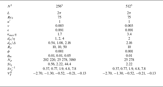
A summary of the set-up parameters is given in table 2. These parameters were chosen to target the coastal sediment transport parameter space wherein the particles are only slightly heavier than the fluid and particle sizes are comparable to the Kolmogorov scale. To this end, Stokes numbers of
 $St_{\eta }=0.56$
,
 $2.22$
and
 $44.4$
and normalised turbulence intensities of
 $Sv_{\ell }^{-1}=0.37$
,
 $0.77$
,
 $1.9$
,
 $4.8$
and
 $7.8$
are tested, resulting in a total of 15 particle-laden cases and one unladen case. The parameters were chosen to represent a wide range of conditions typically observed in the coastal settings. Stokes number and normalised turbulence intensity are varied by changing particle parameters and gravity, which in turn modifies the terminal settling speed in quiescent fluid. The benefit of modifying the particle parameters is that all cases begin from the same turbulent initial conditions, as the actual turbulence intensity remains the same. It should be noted that
 $u^{\prime }/V^0_T$
can also be varied by increasing the turbulence intensity and hence the Reynolds number. However, increasing the Reynolds number, although theoretically feasible, would increase the grid resolution requirement. In addition, with increased
 $Re_{\lambda }$
, the Kolmogorov scale, and hence the particle size, will decrease to obtain Kolmogorov-scale particles. This will in turn increase the number of particles, even for low volume loadings. By changing the particle parameters (size, density), evaluation of how different Stokes number particles respond to varying levels of turbulence intensity relative to the terminal settling speeds was performed. Future work will investigate the effect of
 $Re_{\lambda }$
.
Flow and particle parameters corresponding to homogeneous isotropic turbulence cases where all dimensional parameters are in arbitrary units. Here,
 $N^3$
is the total number of computational grid cells in the cubic domain,
 $L$
is the domain length,
 $Re_{\lambda } \equiv u'\lambda /\nu = 2k/\sqrt {5/3\nu \epsilon }$
is the Taylor-microscale Reynolds number,
 $\lambda$
is the Taylor microscale,
 $\nu$
is the fluid kinematic viscosity,
 $u' \equiv \sqrt {2k/3}$
is the root mean square of fluctuating fluid velocity,
 $k$
is the turbulent kinetic energy,
 $\epsilon$
is the dissipation rate,
 $\kappa _{max}=\pi /\varDelta$
is the maximum resolved wavenumber for grid size
 $\varDelta$
,
 $\eta \equiv (\nu ^3/\epsilon )^{1/4}$
is the Kolmogorov length scale,
 $d_p$
is the particle diameter,
 $R_{\rho }$
is the particle-to-fluid density ratio,
 $\phi$
is the volume loading,
 $\phi _m$
is the mass loading,
 $N_p$
is the total number of particles,
 $St_{\eta }$
is the Stokes number,
 $Sv_{\ell }^{-1}$
is the inverse of the settling parameter, i.e. normalised turbulence intensity, and
 $V_T^0$
is the terminal settling speed in quiescent fluid. The
 $512^3$
cases represent the grid-refinement study for
 $St_{\eta }=2.22$
.

The volume loading in the turbulence cases is limited to
 $\phi =0.001$
in order to maximise the number of particles in the domain while being able to neglect particle-to-particle interactions, thus remaining in a two-way-coupled regime. The purpose of this is to isolate the effects that the turbulence has on the settling particles and not necessarily consider inter-particle effects such as hindered settling, which will be the focus of a future study. Since the density ratios considered are small, the mass loading for all cases is reasonably small (
 $0.01$
–
 $0.05$
) and particles do not significantly modify the global turbulent kinetic energy; however, local effects can still be significant, especially because the particle sizes are comparable to the Kolmogorov scale.
For the Reynolds number studied in the present work, a small-scale resolution of
 $\kappa _{max}\eta \approx 1.7$
, where
 $\kappa _{max}=\pi /\varDelta$
is the maximum wavenumber for grid-size
 $\varDelta$
(Yeung & Pope Reference Yeung and Pope1988; Balachandar & Maxey Reference Balachandar and Maxey1989), is used. The grid resolution used in the present method is similar to the work of Bassenne et al. (Reference Bassenne, Urzay, Park and Moin2016), wherein they used a resolution of
 $\kappa _{max} \eta =1.5$
(
 $384^3$
for
 $Re_{\lambda } = 110$
). Their work is based on second-order, finite-difference scheme based on energy-conserving principles, similar to the one used in the present work. The accuracy of these finite-volume, finite-difference methods will indeed be lower than the spectral methods. However, to ensure that the resolution used is sufficient to capture the turbulence statistics and particle statistics of interest, mainly the particle settling speed and the fluid velocity sampled by the particles, the medium Stokes number case
 $St_{\eta } = 2.22$
was also simulated on a grid resolution that is twice finer in all directions (
 $512^3$
,
 $\kappa _{max} \eta = 3.4$
and maintaining the Courant-Friedrichs-Lewy (CFL) number by reducing the time step) for the five normalised turbulence intensity (
 $u^{\prime }/V_T^0$
) cases. As shown later, the mean settling speeds on the finer mesh are consistent with the coarser mesh settling speeds and the differences are small and well within the standard deviation. In addition, a detailed verification and validation of the numerical predictions and the model used in the present work is conducted as described in Appendix A. A successive mesh refinement study spanning
 $\kappa _{max}\eta _0 = 1.5$
to
 $6.0$
for a decaying isotropic turbulence was conducted for a similar Reynolds number as that studied in the present work. Detailed statistics for turbulent kinetic energy, velocity-derivative skewness, particle kinetic energy, net dissipation rate, particle root mean square acceleration, amongst others, show consistent results between the coarser and finer meshes, as described in Keane et al. (Reference Keane, Apte, Jain and Khanwale2023), with select results also shown in Appendix A. This verifies the adequacy of the grid resolution as well as consistency of particle–fluid interpolation kernels and numerical models under refinement. A coarser mesh was chosen as a compromise between computational efficiency and accuracy.
Particles are initialised with a random position and velocity equal to the local fluid velocity. Simulations are allowed to run for
 $20\tau _{\ell }$
before any statistics are collected, where
 $\tau _{\ell } \equiv \ell /u'$
is the large-eddy-turnover time and
 $\ell \equiv k^{3/2}/\epsilon$
is the integral length scale. After that point, statistics are collected and averaged over
 $(50$
-
 $70)\tau _{\ell }$
in order to have sufficiently converged statistics, as also suggested by Tom et al. (Reference Tom, Carbone and Bragg2022). For fluid tracers in the unladen case, tracer trajectories are stored over a
 $20\tau _{\ell }$
window. For analysis involving spatial data, i.e. the wavelet analysis discussed later, full three-dimensional data and corresponding particle data are stored at ten evenly distributed time steps covering the span of one large-eddy-turnover time at the end of the simulation.
As a consequence of having particles settling through a periodic domain, the mean fluid velocity is reset to zero in each direction at each time step, following previous studies (Bosse et al. Reference Bosse, Kleiser and Meiburg2006; Monchaux & Dejoan Reference Monchaux and Dejoan2017; Rosa et al. Reference Rosa, Kopeć, Ababaei and Pozorski2022; Tom et al. Reference Tom, Carbone and Bragg2022). In the direction of gravity, this is equivalent to imposing a mean vertical pressure gradient. Without this step, the particles and fluid would continually accelerate due to gravity in the absence of solid boundaries.
3. Results and discussion
In this section, the results on the particle settling dynamics in (i) a steady Taylor–Green vortex array and (ii) homogeneous isotropic turbulence are described in detail. For the Taylor–Green case, one-way coupling is used. Visual inspection of the particle trajectories is first provided, followed by statistics on preferential sampling of the vertical fluid velocity as well as the second invariant of the velocity gradient tensor. For the turbulence case, a multiscale analysis of the particle trajectory curvature, sampled vertical fluid velocity and the second invariant of the velocity gradient tensor is performed.
3.1. Taylor–Green vortex
Figure 2 shows the trajectories of particles for three different normalised vortex strengths,
 $U_0/V_T^0=0.2$
,
 $1$
and
 $8$
, for a Stokes number of
 $St=0.6$
. For vortex strength of
 $U_0/V_T^0=0.2$
, the flow is too weak relative to the particle terminal settling speed to cause any meaningful alterations to the particle trajectory, as seen in figure 2(a). For
 $U_0/V_T^0=1$
, the vortex strength equals the terminal settling speed in quiescent fluid. The particle goes through a cycle of downward flow velocity where the particle picks up more speed, making it unable to redirect as it approaches upwards flow velocity regions. The flow is strong enough to alter particle paths, but the particles have enough inertia to not always follow the flow. This results in a loitering behaviour, as seen in figure 2(b), where particles tend to spend more time travelling through upward directed flow regions and less time in the downward directed flow. This longer sampling time of upward directed flow results in a bias towards slower settling speeds. Finally, when the vortex strength is large, corresponding to
 $U_0/V_T^0=8$
, the fluid flow is strong enough to direct the particle through the path of least resistance. The vortices have much higher velocity than the particle terminal speed, and the fluid pushes particles towards downward moving flow, resulting in a clear representation of fast tracking, as seen from figure 2(c). This results in increased settling speed as the particle rarely sees upward moving fluid.
Particle trajectories in a steady, two-dimensional Taylor–Green vortex array for
 $St=0.6$
with normalised vortex strengths of (a)
 $U_0/V_T^0 = 0.2$
, (b)
 $U_0/V_T^0 = 1.0$
and (c)
 $U_0/V_T^0 = 8.0$
.

Normalised settling speed of particles in Taylor–Green vortex array as a function of normalised vortex strength shown for five different Stokes numbers. Shaded region around each line represents
 $\pm$
one standard deviation.

The effect that these observed mechanisms have on the settling speed of the particles is seen in figure 3. The mean settling speed,
 $\langle V_S \rangle$
, normalised by the terminal settling speed in quiescent flow,
 $V_T^0$
, as a function of the normalised vortex strength,
 $U_0/V_T^0$
, is shown for all five Stokes numbers. It is clear that the general trend persists regardless of Stokes number, with some slight differences in the amount of increase or decrease in settling speed at a given normalised vortex strength. For weak vortex strengths, for example
 $U_0/V_T^0=0.2$
, the settling speed of the particle is not altered, which agrees with the observation in figure 2(a) that the flow is too weak to alter the particle trajectory. The particle simply settles straight through the vortices, and despite spending time sampling upwards directed flow velocities, the weak flow is unable to slow down the particle on average. For moderate vortex strengths,
 $U_0/V_T^0 \approx 0.5$
–
 $2$
, the particle trajectories are altered. The particle samples the upward moving fluid for longer periods than the downward moving fluid, thus decreasing the particle settling speed due to this loitering effect seen in figure 2(b). For strong vortex strengths,
 $U_0/V_T^0 \gtrsim 3$
, the particle preferentially samples the downward moving fluid and rarely sees the upward moving fluid, as seen in figure 2(c). This preferential sampling results in fast tracking and enhanced settling speeds.
Mean and standard deviation of sampled non-dimensionalised fluid velocity,
 $\tilde {v}^p = v^p/U_0$
, obtained from the idealised Taylor–Green vortex cases.

3.1.1. Sampled vertical fluid velocity
In the point-particle model, force closures are defined using the undisturbed fluid velocity at the particle location, for example see the standard drag closure (2.4). The only way in which the converged mean settling speed of a particle may differ from it’s terminal settling speed in quiescent flow is by sampling a non-zero undisturbed vertical fluid velocity on average, i.e.
 $\langle v^u(\boldsymbol{x}_p(t),t) \rangle \neq 0$
, where
 $v^u(\boldsymbol{x},t)$
is the component of undisturbed fluid velocity in the direction of gravity (Tom & Bragg Reference Tom and Bragg2019). In a one-way-coupled simulation, where the particle effect on the fluid is not considered, this undisturbed fluid velocity is the main fluid velocity solved for in the model, i.e.
 $v^u(\boldsymbol{x}_p(t),t) = v(\boldsymbol{x}_p(t),t)$
, which for shorthand will be expressed as
 $v^p$
. The mean and standard deviation of non-dimensionalised sampled velocity,
 $\tilde {v}^p = v^p/U_0$
, for the idealised Taylor–Green vortex cases is given in table 3. The values in the table are non-dimensionalised in order to allow comparison of the mean and standard deviation between cases which have different characteristic length and velocity scales. Comparing trends in figure 3 with values in table 3, it can be seen that the cases which experience decreased settling speeds relative to their terminal settling speed in quiescent fluid have
 $\langle v^p \rangle \gt 0$
, while those that experience enhanced normalised settling speeds have
 $\langle v^p \rangle \lt 0$
. Further insight into the subtleties of this statistic can be gained by examining the probability density functions (PDFs) of
 $v^p$
. Figure 4 shows the PDFs of
 $v^p$
for
 $St=0.1$
, 0.6 and 2.0 and
 $U_0/V_T^0=0.2$
, 1.0 and 8.0. This subset of cases represents the most distinct settling behaviours. For all Stokes numbers,
 $U_0/V_T^0=0.2$
shows essentially no modification in settling rate relative to the terminal settling speed in quiescent fluid,
 $\langle v^p \rangle \approx 0$
indicating a uniform sampling of vertical fluid velocities, and the PDF is nearly identical to that of a fluid tracer. The cases with
 $U_0/V_T^0=1$
all experienced decreased settling speeds with
 $\langle v^p \rangle \gt 0$
, meaning that the particles sampled more upwards directed fluid velocity on average. In the PDFs, it is clear that these particles do sample both negative and positive vertical fluid velocities, but the magnitude of the positive sampling is much greater, thus skewing the average. This is evidence of loitering, where particles sample both directions of flow, but due to the opposing flow reducing settling speeds, the particles spend more time in this upwards directed flow region, thus biasing the average sampling towards that positive vertical fluid velocity and reducing the mean normalised settling speed. Finally, for
 $U_0/V_T^0=8$
, all Stokes numbers see enhanced settling speeds which go in hand with
 $\langle v^p \rangle \lt 0$
, i.e. the particles spend more time sampling downwards directed fluid velocity than upwards. The PDFs support this as well, showing barely any sampling of upwards directed fluid velocity relative to the amount of downward directed flow sampling. This is corroborated with the plot of trajectories in figure 2 and the fast tracking mechanism, where the particles are essentially constantly moving towards downward directed fluid velocities, thus enhancing their settling speeds.
Probability density functions of
 $v^p$
, normalised by it’s standard deviation, for (a)
 $St = 0.1$
, (b)
 $St = 0.6$
and (c)
 $St = 2.0$
particles settling through a steady, two-dimensional Taylor–Green vortex array.

3.1.2. Preferential sampling of the flow
Next, the particle-sampled second invariant of the velocity gradient tensor,
 $\mathcal{Q}^p(t)$
, is examined to show how it relates to what is seen in the particle trajectories of the Taylor–Green vortex cases. The second invariant of the velocity gradient tensor is given as
 \begin{align} \mathcal{Q} = -\frac {1}{2}A_{ik}A_{ik} = \frac {1}{4}\omega _i \omega _i - \frac {1}{2}S_{ij}S_{ij}, \end{align}
where
 $\unicode{x1D63C}$
is the velocity gradient tensor,
 $\boldsymbol{\omega }$
is vorticity, and
 $\unicode{x1D64E}$
is the strain-rate tensor. This scalar quantity represents a balance between enstrophy and strain-rate-squared magnitude (Johnson & Wilczek Reference Johnson and Wilczek2024). It follows from this balance that regions of the flow dominated by high strain-rate would exhibit
 $\mathcal{Q}\lt 0$
, while regions dominated by high vorticity, and hence enstrophy, would exhibit
 $\mathcal{Q}\gt 0$
. In the case of particle-laden flow, one can examine how the particles sample this scalar field,
 $\mathcal{Q}^p(t)=\mathcal{Q}(\boldsymbol{x}_p(t),t)$
, in order to determine where in the flow the particles spend time. Average particle behaviour, such as fast tracking or vortex trapping, can be determined by averaging this quantity across all particles and all time over a set statistically stationary period. Particles experiencing vortex trapping would naturally sample vorticity dominated regions of the flow, which would be evidenced by
 $\langle \mathcal{Q}^p(t) \rangle \gt 0$
, while particles experiencing fast tracking move between regions of high strain rate, which would be seen as
 $\langle \mathcal{Q}^p(t) \rangle \lt 0$
. In the case of uniform sampling, when particles behave much like fluid tracers,
 $\langle \mathcal{Q}^p(t) \rangle = \langle \mathcal{Q}(t) \rangle$
, which in a homogeneous flow equals zero.
Mean and standard deviation of non-dimensionalised second invariant of the velocity gradient tenor,
 $\tilde {\mathcal{Q}}^p = \mathcal{Q}^p / (U_0^2/D_v^2)$
, obtained from the idealised Taylor–Green vortex cases. Corresponding values for fluid tracers are
 $\langle \tilde {\mathcal{Q}}^p \rangle \approx -0.08$
and
 $\sigma ( \tilde {\mathcal{Q}}^p ) \approx 4.96$
.

The mean and standard deviation of non-dimensionalised
 $\tilde {\mathcal{Q}}^p = \mathcal{Q}^p/(U_0^2/D_v^2)$
for all Taylor–Green vortex cases are given in table 4. The values in the table are non-dimensionalised in order to allow comparison of mean and standard deviation between cases which have different characteristic length and velocity scales. For all Stokes numbers and vortex intensities tested here,
 $\langle \tilde {\mathcal{Q}}^p \rangle \lt 0$
, which indicates that to some extent the particles spend more time in higher strain-rate regions of the flow. However, the absolute value of this mean needs to be compared with its standard deviation in order to infer the extent of preferential sampling. In general, for the weakest vortex intensity cases, which show little to no modification of mean settling speeds, the standard deviation of
 $\tilde {\mathcal{Q}}^p$
is larger than other cases and the absolute value of the mean is small compared with that standard deviation. The larger standard deviation is a result of slightly more uniform sampling of the flow and having a small absolute value mean relative to this standard deviation indicates that the level of preferential sampling is very small relative to the spread of sampled regions of the flow. For
 $U_0/V_T^0=1$
, the cases which showed reduced settling speeds, the standard deviation of
 $\tilde {\mathcal{Q}}^p$
decreases as particles concentrate more so onto the vertical loitering paths, as can be seen in figure 2(b). The ability of the particles to converge onto these vertical loitering paths is dependent on Stokes number, with the
 $St=0.1$
particles being more reactive to the fluid and thus not taking as straight paths through the vortices and the
 $St=2$
particles carrying more inertia and thus not as easily or quickly converging onto these set vertical paths. This is consistent with these two cases having slightly larger standard deviations of
 $\tilde {\mathcal{Q}}^p$
than the in between Stokes numbers for
 $U_0/V_T^0=1$
, as well as having the smallest amount of settling speed reduction at this vortex intensity, as seen in figure 3. For
 $U_0/V_T^0 \geqslant 3$
, as the vortex intensity increases, the standard deviation of
 $\tilde {\mathcal{Q}}^p$
decreases while the absolute value of the mean increases. This trend indicates that the spread of sampled regions of the flow is getting smaller and the particles are increasingly sampling high strain-rate flow regions, resulting in more efficient fast tracking which leads to the enhanced settling speeds seen in figure 3.
Probability density functions of
 $\mathcal{Q}^p$
, normalised by it’s standard deviation, for (a)
 $St = 0.1$
, (b)
 $St = 0.6$
and (c)
 $St = 2.0$
particles settling through a steady, two-dimensional Taylor–Green vortex array.

Deeper insights into the dynamics of these particles and how they sample the flow can be gained by examining the full PDFs and comparing them with the fluid tracer case. The PDFs of
 $\mathcal{Q}^p(t)$
for cases with
 $St=0.1$
, 0.6 and 2, along with a reference line for the fluid tracers, normalised by their standard deviation, are shown in figure 5. Lines for
 $U_0/V_T^0=0.2$
, 1.0 and 8.0 are shown as they represent the three most distinct settling trends, while the other cases are once again omitted from these plots for brevity. Starting with
 $U_0/V_T^0=0.2$
, for all Stokes numbers, the settling speed was not modified much due to the relatively weak flow. This results in particles sampling all parts of the flow uniformly as they settle more or less straight through the vortices, which is observed in the PDF remaining fairly close to the fluid tracer PDF. When
 $U_0/V_T^0=1$
, all Stokes numbers observe a reduction in settling speeds. For
 $St=0.1$
and 0.6 in figure 5(a,b), the particles in the
 $U_0/V_T^0=1$
cases sample more high strain-rate and high vorticity regions than the fluid tracers, indicated by the tails extending further in each direction. However, this is accompanied by less sampling of moderate strain-rate and vorticity regions than fluid tracers and also a larger peak near zero, indicating no preferential sampling of either region. Even though there is some sampling of high strain-rate regions of the flow, the trajectories in figure 2(b) show that this is due to particles taking more straight vertical paths between vortices, resulting in loitering. For this same normalised vortex strength, the
 $St=2$
case is slightly different. As observed in figure 3, the settling speed for
 $St=2$
when
 $U_0/V_T^0=1$
is not reduced as much as for smaller Stokes numbers, thus the difference in the PDF relative to the fluid tracers is not as significant. Now, considering the cases which see enhanced settling speeds, visualised for
 $U_0/V_T^0=8$
, there are notable differences in figure 5. For all Stokes numbers, these vortex strengths correspond with the largest sampling of strain-rate dominated flow in conjunction with extremely low sampling of vorticity dominated regions, resulting in efficient fast tracking.
These idealised Taylor–Green vortex cases provide visual examples of the mechanisms in which particle settling speeds may be altered by turbulence, namely fast tracking and loitering for the parameter space of interest. By examining this statistic in conjunction with the visual trajectories, one can discern the settling pattern and mechanisms of particles. These analysis techniques are applied to particle settling in homogeneous, isotropic turbulence in the next section.
3.2. Homogeneous, isotropic turbulence
In this section, the dynamics of sediment-like particles settling through homogeneous, isotropic turbulence for three Stokes numbers, and how they change as a function of normalised turbulence intensity,
 $Sv_{\ell }^{-1}=u'/V_T^0$
, are examined. It should be noted again that the averaged statistics discussed here were averaged over a minimum of
 $50\tau _{\ell }$
, which was shown to be a sufficient window for obtaining statistically stationary results for these cases.
The normalised settling rates for each turbulence case are shown in figure 6. In all cases, the smaller normalised turbulence intensities result in no significant changes to settling rates over the terminal settling speed in quiescent fluid, as expected for the relatively weak flows. As turbulence intensity is increased relative to the still-water terminal settling speed, there are two main trends that are clearly observed. The cases with
 $St_{\eta }=0.56$
and 2.22 both experience only enhanced settling rates, while the
 $St_{\eta }=44.4$
cases experience only reduced settling rates. Thus, there are clearly different mechanics at play between the low-to-moderate Stokes number and the high Stokes number cases. These trends are also quite different from the idealised Taylor–Green vortex array cases, as seen in figure 3. These differences could be attributed to the fact that, in turbulence, eddies are constantly moving and changing and so the path that particles take throughout the turbulent field cannot be as well defined as in the steady vortex array sheet. Therefore, the way in which certain particles interact with the turbulent eddies, whether through loitering, fast tracking or other mechanisms, could be very different for a given parameter space. However, the main concept of these mechanisms and the interpretation of the statistics used to identify them remain unchanged.
Normalised settling speed of particles settling in homogeneous isotropic turbulence as a function of normalised turbulence intensity for three different Stokes numbers. Shaded region around each line represents
 $\pm$
one standard deviation. The dashed line with hollow diamond markers represents the same
 $St_{\eta }=2.22$
case computed on the finer resolution (
 $512^3$
). Inset shows results obtained using the particle self-disturbance correction model (filled markers) compared with those from an uncorrected model (hollow markers) for the
 $St_{\eta }=0.56$
case.

3.2.1. Effect of self-disturbance correction and two-way coupling
In order to highlight the importance of correcting for the particle self-disturbance in the point-particle force closures for particle sizes of the order of the Kolmogorov scale, the inset in figure 6 shows the normalised settling rates for
 $St_{\eta }=0.56$
comparing results with and without the particle self-disturbance correction. Table 5 provides the corresponding percentage difference in the mean settling speed compared with that in quiescent flow obtained with and without correction. The uncorrected simulation shows much further enhanced settling rates for all normalised turbulence intensities. In the uncorrected model, the particle disturbances are propagated through the two-way-coupled fluid velocity into the modelled particle forces. Consequently, a lower value for the slip velocity at the particle location is obtained compared with predictions with the correction model, which in turn results in lower drag and higher settling speeds. This result indicates that the artificial increase in settling speed of sediment-like particles resulting from the use of disturbed fluid velocities in force closures can be significant.
Percentage change in mean settling speed, relative to terminal settling speed in quiescent flow, i.e.
 $(({\langle V_S \rangle - V_T^0})/{V_T^0})\times 100\,\%$
comparing the two–way-coupled MRG model with zonal-ADR correction, one-way coupled and two-way coupled without any correction for self-disturbance.

Furthermore, for the low Stokes number, simulations were also performed with one-way coupling and compared with the two-way coupling prediction with self-disturbance correction. The one-way-coupled settling rates were also higher by up to 9.5 %. With two-way coupling, even though the self-disturbance is removed to obtain the undisturbed fluid velocity at the particle location, it still contains the effect of neighbouring particles by definition. For the Kolmogorov-scale particles studied here, it is found that this effect results in lower settling speeds. Tom et al. (Reference Tom, Carbone and Bragg2022) conducted a detailed study comparing one-way- and two-way-coupled particles settling in isotropic turbulence. They show increased settling speeds compared with one-way coupling. However, in their work particles were much heavier and sub-Kolmogorov scale and also they did not consider any correction for the self-disturbance created by the particle.
It is clear that, even for the low Stokes number case, two-way coupling effects alter the local fluid flow, which in turn influences the mean settling speeds. A more detailed comparison of one-way versus two-way coupling with corrections for the self-disturbance velocity field should be conducted for all Stokes numbers and will be the focus of future work.
3.2.2. Effect of Basset history force
For the low density ratio particles considered in the present work, the history force can have a significant effect on the particle settling speeds. The history force typically affects the particle response time (Jaroslawski et al. Reference Jaroslawski, Jaganathan, Govindarajan and McKeon2024) and also the settling speed (Li et al. Reference Li, Bragg and Katul2023). This was examined by computing all cases with and without the use of the Basset history force, as shown in table 6.
Percentage change in mean settling speed, relative to terminal settling speed in quiescent flow, i.e.
 $(({\langle V_S \rangle - V_T^0})/{V_T^0})\times 100\,\%$
with and without the Basset history force. Both cases implemented two-way coupling with the zonal-ADR correction scheme.

For the
 $St_{\eta } = 0.56$
case, which resulted in settling speed enhancements with increasing normalised turbulence intensity, the exclusion of the history force generally resulted in slightly larger increases in settling speed. For the
 $St_{\eta } = 44.4$
case, which showed decreased settling speeds with increasing normalised turbulence intensity, the inclusion of the history force diminished this percentage decrease. This effect was more pronounced at large normalised turbulence intensities. These observations point to the fact that the history force causes particles to relax to the terminal speed slower, effectively increasing their response time. Thus, they tend to react slowly to surrounding fluid flow fluctuations, affecting the fast tracking or loitering mechanisms. This observation is consistent with the work of Li et al. (Reference Li, Bragg and Katul2023). For the medium Stokes number, the impact of including the history force was slightly more minimal.
3.2.3. Sampled vertical fluid velocity
In the idealised one-way-coupled Taylor–Green vortex case, the vertical fluid velocity seen by a particle had a simple interpretation: a particle that spends more time in downwards moving flow experiences enhanced settling rates and vice versa. However, in the homogeneous, isotropic turbulence cases, this interpretation is not so straightforward, as the flow is two-way coupled, and more importantly, the particles are of the order of the smallest flow scales. Because of this, the fluid velocity at the particle location is the disturbed fluid velocity. As discussed previously, this is accounted for within the model, and the self-disturbance created by each particle is removed when calculating particle forces, however, since each particle has a unique undisturbed flow associated with it, the flow used for the following analysis is the regular two-way-coupled flow containing all particle disturbances. Since homogeneous, isotropic turbulence is characterised by a range of length and time scales, it is desirable to be able to examine how particles interact with different flow scales. To this end, multiscale wavelet analysis of the fluid flow sampled by the particles as well as the second invariant of the velocity gradient tensor is performed. The wavelet analysis facilitates decomposing the velocity field into multiple fields, each characterised by a specific band of flow scales. The present analysis is performed on the full two-way-coupled fluid velocity, which allows identification of which flow scales impact the particle dynamics most as well as which flow scales are directly affected by the particle. This is similar to the multiscale analysis of two-way-coupled flow field conducted by Tom et al. (Reference Tom, Carbone and Bragg2022), except that they explicitly filtered the flow field at different scales. The wavelet analysis (detailed below), on the other hand, provides information on specific bands of scales in the multiscale decomposition, and allows easy evaluation of flow scales interacting with the particles. The mean and standard deviation of this sampled, unfiltered, vertical fluid velocity,
 $v(\boldsymbol{x}_p)$
, is given in table 7, for reference. When examining the multiscale statics of two-way-coupled fluid velocity at the particle location, the effect of the particle self-disturbance, as well as neighbouring particle effects, will be present.
Mean and standard deviation of
 $v^p$
obtained from the unfiltered fluid field in the homogeneous, isotropic turbulence cases.

For comprehensive details regarding wavelet analysis, see Mallat (Reference Mallat2009), Schneider & Vasilyev (Reference Schneider and Vasilyev2010) and Farge & Schneider (Reference Farge and Schneider2015). Consider the two-way-coupled vertical fluid velocity,
 $v(\boldsymbol{x},t)$
, at a given time
 $t$
, within the triply periodic cubic domain of size
 $(2\pi )^3$
. This scalar field is decomposed into a three-dimensional (3-D) orthogonal wavelet series to unfold into scale, positions and seven directions (
 $\mu = 1,2,\dots , 7$
). The 3-D mother wavelet,
 $\psi _{\mu }(\boldsymbol{x})$
, is hereby based on a tensor product construction and a family of wavelets,
 $\psi _{\mu ,\boldsymbol{\lambda }}(\boldsymbol{x})$
, can be generated by dilation and translation. The multi-index
 $\boldsymbol{\lambda }=(j,i_1,i_2,i_3)$
denotes the scale
 $2^{-j}$
and position
 $2\pi \times 2^{-j}\boldsymbol{i} = 2\pi \times 2^{-j}(i_1,i_2,i_3)$
of the wavelets for each direction, where
 $i_{\ell }=0,\dots ,2^{j}-1$
 $(\ell =1,2,3)$
. The wavelets are well localised in space around position
 $2\pi \times 2^{-j}\boldsymbol{i}$
and scale
 $2^{-j}$
, oscillating and smooth. A periodisation technique (Mallat Reference Mallat2009) is applied to the wavelets. The spatial average of
 $\psi _{\mu ,\boldsymbol{\lambda }}(\boldsymbol{x})$
, defined by
 $\langle \psi _{\mu ,\boldsymbol{\lambda }} \rangle = (2\pi )^{-3}\int _{\mathbb{T}^3}\psi _{\mu ,\boldsymbol{\lambda }}(\boldsymbol{x})d\boldsymbol{x}$
, vanishes for each index, which is a necessary condition for being a wavelet.
The vertical fluid velocity,
 $v(\boldsymbol{x})$
, sampled on
 $N^3=2^{3J}$
equidistant grid points, can be developed into an orthogonal wavelet series
 \begin{equation} v(\boldsymbol{x}) = \langle v(\boldsymbol{x}) \rangle + \sum _{j=0}^{J-1} v_j(\boldsymbol{x}), \end{equation}
where
 $v_j(\boldsymbol{x})$
is the contribution to
 $v(\boldsymbol{x})$
at scale
 $2^{-j}$
, defined by
 \begin{equation} v_j(\boldsymbol{x}) = \sum _{\mu =1}^{7} \sum _{i_1,i_2,i_3=0}^{2^j-1}\widetilde {v}_{\mu ,\boldsymbol{\lambda }}\psi _{\mu ,\boldsymbol{\lambda }}(\boldsymbol{x}), \end{equation}
with the coefficients given by
 $\widetilde {v}_{\mu ,\boldsymbol{\lambda }}=\langle v, \psi _{\mu ,\boldsymbol{\lambda }}\rangle$
, where
 $\langle \cdot , \cdot \rangle$
denotes an inner product. At scale
 $2^{-j}$
, there are
 $7\times 2^{3j}$
wavelet coefficients for
 $v(\boldsymbol{x})$
. Thus, in total there are
 $N^3$
wavelet coefficients for each component of the vector field corresponding to
 $N^3-1$
wavelet coefficients and the non-vanishing mean value. These coefficients are efficiently computed from the
 $N^3$
grid points for
 $v(\boldsymbol{x})$
using the fast wavelet transform. The
 $2^{-j}$
scale from the wavelet transform and wavenumber,
 $k_j$
, from the Fourier transform are related as
 \begin{equation} k_j = k_{\psi }2^j, \end{equation}
where
 $k_{\psi }$
is the centroid wavenumber of the chosen wavelet. In the present study, we use the Coiflet 12 wavelet, which has
 $k_\psi = 0.77$
. Figure 7(a) shows instantaneous
 $v(\boldsymbol{x})$
contours, normalised by their standard deviation, in the
 $xy$
-plane for
 $St_{\eta }=2.22$
and
 $u'/V_T^0=0.37$
. The instantaneous
 $v(\boldsymbol{x})$
field is decomposed using the orthogonal wavelet transform discussed above and a few representative scale-dependent fields,
 $v_j$
, normalised by their standard deviation, are shown in figure 7(b)–7(d). The small-scale structures in figure 7(d) correspond to around 2.4 times the particle diameter. The effect of two-way coupling due to settling particles, which depends on the particle distribution and their number density in the computational domain, tends to mostly influence the velocity fluctuations on these small scales, resulting in the two-way coupling signature observed here.
Instantaneous 2-D slice of vertical fluid velocity normalised by its standard deviation,
 $v/\sigma (v)$
, (a) and scale contributions
 $v_j/\sigma (v_j)$
at
 $k_j\eta = 0.02$
(b),
 $k_j\eta = 0.08$
(c) and
 $k_j\eta = 0.66$
(d) for
 $St_{\eta }=2.22$
and a normalised turbulence intensity of
 $u'/V_T^0=0.37$
.

In order to determine the flow scales that interact with the particles the most, the different scale contributions sampled by the particles are examined for the vertical fluid velocity,
 $v(\boldsymbol{x})$
, i.e.
 $v_j^p = v_j(\boldsymbol{x}_p)$
. For each scale contribution, the mean of this quantity,
 $\langle v_j^p \rangle$
, can be obtained along with any higher-order statistics. Since this two-way-coupled fluid velocity contains the particle disturbance on the flow, the interpretation of this mean quantity must be looked at as containing both the effect of the particle disturbance on the flow at that scale as well as the part of the flow being sampled by the particle. Since particle disturbances are largest very near the particle, it is likely that the smaller scales are most affected by the particle, while this disturbance would be less likely to affect the larger scales. These scale contributions to
 $v^p$
are shown in figure 8. To relate the scales shown to the actual eddy sizes, the wavenumber scale can be converted to eddy diameter as follows:
 $k_j\eta = (\pi /D)\eta$
, where
 $D$
is the diameter of the eddy associated with a particular scale. For
 $St_{\eta }=0.56$
, the biggest influence on the vertical fluid velocity appears to occur for the smallest wavelet scale,
 $k_j\eta = 1.309$
. Following the conversion, and knowing that
 $\eta =d_p$
in this low Stokes number case,
 $1.309 = (\pi /D)\eta = (\pi /D)d_p$
, thus the peak influence on vertical fluid velocity at the particle location corresponds to eddies of diameter
 $D\approx 2.4d_p$
, and this influence drops off for larger scales. In the
 $St_{\eta }=2.22$
case, the largest influence of particles on the vertical fluid velocity occurs around eddies of diameter
 $D\approx 2.4d_p$
as well, which is consistent with the lower Stokes number case. For
 $St_{\eta }=44.4$
, aside from the peak at large flow scales in the
 $u'/V_T^0=0.37$
case, which will be discussed later, the biggest influence on vertical fluid velocity at the particle location is again at scales corresponding to eddies of diameter
 $D\approx 2.4d_p$
. Thus, the flow scale most affected by the presence of particles seems to be consistently proportional to the particle diameter, and is 2.4 times the diameter for the cases studied. Since the wavelet decomposition provides flow structures at scales separated by a power of two, this size relationship should be considered an estimate and not a precise ratio.
Contributions to vertical fluid velocity sampled by the particle,
 $v^p$
, by different flow scales for (a)
 $St_{\eta }=0.56$
, (b)
 $St_{\eta }=2.22$
and (c)
 $St_{\eta }=44.4$
, normalised by the standard deviation of the unfiltered values. Inset plots show scale contributions to
 $v^p$
with each scale normalised by the scale-specific standard deviation, i.e.
 $-\langle v_j^p \rangle / \sigma (v_j^p)$
. Vertical dashed reference lines indicate the particle-size scale.

For all of these Stokes numbers, the effect on fluid velocity at these smaller scales increases for decreasing normalised turbulence intensity, because as the flow gets weaker relative to the terminal settling speed, it becomes less effective at wiping out particle disturbances. Another way to think of this is that inertial particles create wakes as they travel through the flow, and if the turbulence is strong enough relative to the terminal settling speed, it can essentially smear out the wake. However, for weaker turbulence, the wake may persist for longer, making for a more evident effect on the vertical fluid velocity at the particle location. In the low and moderate Stokes number cases,
 $St_{\eta }=0.56$
and 2.22, the two lowest turbulence intensities have less of an average effect at the larger scales. Knowing that the mean settling speeds are relatively unmodified in these cases, this could be consistent with the hypothesis that the particles are more uniformly sampling both upwards and downwards directed flow due to how weak the flow is relative to their settling speeds. The two highest normalised turbulence intensity cases,
 $u'/V_T^0=4.8$
and 7.8, however, show a smaller, yet persistent, effect at all scales for a different reason. In these cases, the particles are preferentially sampling the flow through fast tracking, as evidenced by increased settling speeds in figure 6, and so the smaller mean effect on the vertical fluid velocity is likely due to the stronger normalised turbulence intensity being able to wipe out the particle disturbances more effectively. The
 $u'/V_T^0=1.9$
cases seem to have the largest effect on the vertical fluid velocity towards the moderate and larger scales, likely due to a balance between preferentially sampling downwards directed flow and the turbulence not quite being strong enough to wipe out the particle disturbances as effectively as the higher turbulence intensity cases.
In the
 $St_{\eta }=44.4$
case, the higher turbulence intensities show a near-zero effect on the average vertical fluid velocity at the particle locations because the turbulence is effectively wiping out particle disturbances and the particles are more uniformly sampling the flow through the loitering mechanism. The main difference in behaviour occurs for the weakest normalised turbulence intensity,
 $u'/V_T^0=0.37$
, at the larger flow scales. This case has larger particles,
 $d_p=4\eta$
, which inherently create larger-scale disturbances. It is also the only case with a larger mass loading of
 $\phi _m = 0.05$
, compared with the low and moderate Stokes number cases which had
 $\phi _m = 0.01$
. It is likely that the wakes are large enough, due to the larger particles and increased mass loading, and persistent enough, due to the relatively weak flow, that they can interact with wakes from other particles, building up a larger-scale fluid motion through somewhat of a group effect on the flow. Examining the inset in figure 8(c), the standard deviation of
 $v^p_j$
at those larger scales is much larger than the standard deviation of the unfiltered data, so while the mean scale contribution is a negative large-scale fluid velocity at the particle locations, there is a much wider range of sampled fluid velocities at the large scales compared with other cases. This trend of larger standard deviation at larger scales appears to be consistent among all Stokes numbers. Particles in the
 $St_{\eta }=0.56$
and
 $St_{\eta }=2.22$
cases do not likely create wakes big enough to interact with each other before the turbulence effectively breaks up the wakes, even in the lowest normalised turbulence intensity cases.
While examining the mean vertical fluid velocity associated with different flow scales at the particle location provides useful information on which flow scales seem to be the most affected by particle disturbances, it gives less concrete information on how the flow itself is affecting the settling dynamics of such particles. In a sense, this multiscale fluid velocity analysis provided information mostly from one side of the two-way coupling interaction, but other statistics are needed to provide information on the other side. To accomplish this, the multiscale mean particle trajectory curvature statistics are obtained, which can be used to help provide information on how the particles may be travelling through the fluid relative to the fluid particles or tracers, followed by an additional multiscale analysis on the particle-sampled second invariant of the velocity gradient tensor.
3.2.4. Particle trajectory curvature
When it comes to identifying which mechanisms are responsible for altering particle settling speeds in turbulence, one of the key differences among mechanisms is how the particle trajectories curve throughout the fluid. That is, when particles fast track, they are following the outside edges of eddies, and when particles are vortex trapped, they spin around with the fluid inside these eddies. In contrast to these two mechanisms, when a particle exhibits loitering, it has a tendency to travel in straight paths, going through eddies rather than around them. These key differences in the way particles traverse through the fluid can be examined by measuring the curvature of the particle trajectories compared with that of fluid particles.
Scale-dependent curvature angles of particle trajectories describe how particles move around flow features of different scales and have been described in detail in Bos, Kadoch & Schneider (Reference Bos, Kadoch and Schneider2015) and Kadoch et al. (Reference Kadoch, Bassenne, Esmaily-Moghadam, Schneider, Farge and Bose2016). Using the particle trajectory history, a time increment of the Lagrangian particle position is defined as
 \begin{equation} \delta \boldsymbol{X}(\boldsymbol{x}_0,t,\tau ) = \boldsymbol{X}(\boldsymbol{x}_0,t) - \boldsymbol{X}(\boldsymbol{x}_0,t-\tau ), \end{equation}
where
 $\boldsymbol{X}(\boldsymbol{x}_0,t)$
is the particle position at time
 $t$
, passing through point
 $\boldsymbol{x}_0$
at time
 $t=t_0$
. Using three consecutive points separated by time
 $\tau$
on a particle trajectory, an angle of curvature
 $\Theta (t,\tau )$
can be obtained as
 \begin{equation} \text{cos}(\Theta (t,\tau )) = \frac {\delta \boldsymbol{X}(\boldsymbol{x}_0,t,\tau ) \cdot \delta \boldsymbol{X}(\boldsymbol{x}_0,t+\tau ,\tau )}{|\delta \boldsymbol{X}(\boldsymbol{x}_0,t,\tau )||\delta \boldsymbol{X}(\boldsymbol{x}_0,t+\tau ,\tau )|}. \end{equation}
This quantity provides the angle describing the directional change of a particle in the plane for a given time scale characterised by the increment size
 $\tau$
(Kadoch et al. Reference Kadoch, Bassenne, Esmaily-Moghadam, Schneider, Farge and Bose2016). An ensemble average of these curvature values of all particles over all times gives a mean trajectory curvature angle denoted by
 \begin{equation} \theta (\tau ) \equiv \langle |\Theta (t,\tau )| \rangle . \end{equation}
For fluid tracers in homogeneous, isotropic turbulence,
 $\theta (\tau )$
tends to zero for short lag times
 $\tau$
, which means that the particles have a tendency to go straight for short durations. As the lag time between trajectory points becomes very large, the angle of curvature tends to an asymptotic value of
 $\pi /2$
, corresponding to a decorrelation time between three points, i.e. over this time scale the three points are randomly positioned with respect to each other (Kadoch et al. Reference Kadoch, Bassenne, Esmaily-Moghadam, Schneider, Farge and Bose2016).
Mean particle trajectory curvature angle as a function of lag time scale for (a)
 $St_{\eta }=0.56$
, (b)
 $St_{\eta }=2.22$
and (c)
 $St_{\eta }=44.4$
, compared with fluid tracer trajectory curvature angle (black squares). Dashed reference lines include: horizontal asymptotic value of
 $\pi /2$
, linear scaling reference line at low lag times and vertical reference lines for the ratio between particle relaxation time and Kolmogorov time scale, i.e.
 $St_{\eta }$
, and the ratio between the integral time scale and Kolmogorov time scale.

Figure 9 shows the mean trajectory curvature angle as a function of the lag time, normalised by the Kolmogorov time scale, for sediment-like particles of different Stokes numbers along with the mean trajectory curvature angle of the fluid tracers in the corresponding unladen case. It can be seen that the fluid tracers follow the theoretical trend for fluid trajectory curvature in homogeneous, isotropic turbulence, with
 $\theta (\tau ) \rightarrow 0$
as
 $\tau \rightarrow 0$
, scaling linearly with
 $\tau$
through the small lag times, and reaching an asymptotic value of
 $\pi /2$
at long lag times. The fluid tracer trajectory curvature angle should scale with
 $\tau ^{1/2}$
through the inertial subrange (Bos et al. Reference Bos, Kadoch and Schneider2015), but the Reynolds number of the current simulations is too small to observe a distinct inertial range.
Inertial particle trajectory curvature angles for cases
 $St_{\eta }=0.56$
and
 $St_{\eta }=2.22$
display similar behaviour, as seen in figure 9(a,b). For lower lag times, all normalised turbulence intensities result in a mean particle trajectory curvature roughly equalling the mean fluid trajectory curvature. As lag time increases, the mean curvature angles of particle trajectories in the
 $u^{\prime }/V_T^0=0.37$
and 0.77 cases drop off relative to the fluid trajectory curvature. This is the case of the turbulence being too weak relative to the particle terminal settling speeds, resulting in particles taking more of a straight path through the larger time scale eddies, similar to the Taylor–Green test case trajectories observed in figure 2(a). For these weaker normalised turbulence cases, the flow was too weak to significantly modify the particle settling speed, regardless of the particles having less trajectory curvature than the fluid on average. As the normalised turbulence intensity increases, the mean particle trajectory curvature closely follows the mean fluid trajectory curvature in these low-to-moderate Stokes number cases. This behaviour is indicative of fast tracking and/or vortex trapping, where the particles are closely following fluid particles, similar to the Taylor–Green test case trajectories observed in figure 2(c). These cases result in enhanced settling speeds relative to their terminal settling speed in quiescent fluid, which hints towards fast tracking over vortex trapping, but further statistical analysis will be used to prove this. Looking at the higher Stokes number case in figure 9(c), which saw decreased settling speeds, the mean particle trajectory curvature is much less than the fluid trajectory curvature for all lag times. For these cases, the particle relaxation time scale is larger than the integral flow time scale, suggesting that particles are slow to respond to turbulent flow fluctuations. Again, in the two smaller normalised turbulence intensities, the flow is too weak to significantly modify settling speeds. However, in the larger normalised turbulence intensity cases, this reduced particle trajectory curvature results in reduced settling speeds. Particles having less trajectory curvature than the fluid means that, on average, the particles have a tendency to go through eddies rather than curving around them, similar to the Taylor–Green test case trajectories observed in figure 2(b). In addition, owing to their higher inertia, particles tend to travel in straight lines for longer time compared with the fluid particles. Inevitably, this results in particles spending more time sampling upwards directed fluid velocities than if the particles were matching fluid trajectory curvature. This is evidence of the loitering mechanism which would explain the observed reduced settling speeds.
As mentioned previously, if the particle trajectory curvature matches that of the fluid trajectory curvature, there could still be a couple possibilities as to what mechanism is at play, i.e. both fast tracking and vortex trapping result in particles following the fluid trajectory curvature. While the enhanced settling speeds of the low-to-moderate Stokes number cases highly suggest the fast tracking mechanism, this can be proven by looking at multiscale analysis of the second invariant of the velocity gradient tensor in conjunction with these trajectory curvature results, and is discussed below.
3.2.5. Preferential sampling of the flow
In addition to comparing the mean trajectory curvature angles of particles with that of the fluid, more information can be gained by looking at which parts of the flow are being predominantly sampled by these sediment-like particles. Of interest here is the particle-sampled second invariant of the velocity gradient tensor,
 $\mathcal{Q}^p$
. As discussed in earlier sections, this statistic can elucidate whether the particles are spending more time sampling strain-rate dominated regions of the flow (
 $\mathcal{Q}^p\lt 0$
), vorticity dominated regions of the flow (
 $\mathcal{Q}^p\gt 0$
) or if they are not preferentially sampling the flow in either way (
 $\mathcal{Q}^p=0$
). For reference, the mean and standard deviation of
 $\mathcal{Q}^p$
for each case, including the fluid tracer case, is given in table 8. Initial observations are that every case has a negative mean
 $\mathcal{Q}^p$
, however, the mean values for the
 $St_{\eta }=0.56$
and 2.22 cases are much more negative than the
 $St_{\eta }=44.4$
case. This suggests that low-to-moderate Stokes number particles tend to sample high strain-rate regions of flow more frequently than higher Stokes number particles. In addition, with an increase in turbulence intensity, low and moderate Stokes number particles show larger negative values for
 $\langle \mathcal{Q}^p \rangle$
combined with generally reduced standard deviations, and this is in agreement with the fact that enhanced settling was observed for increased turbulence intensities relative to the particle terminal speed. The one departure from this trend is the weakest turbulence intensity case at these low and moderate Stokes numbers, which has a larger negative
 $\langle \mathcal{Q}^p \rangle$
than some of the moderate turbulence intensity cases, however, this is combined with a larger standard deviation and the knowledge that this level of turbulence intensity is not strong enough to significantly alter settling speeds despite any possible preferential sampling.
Mean and standard deviation of
 $\mathcal{Q}^p$
obtained from the unfiltered fluid field in the homogeneous, isotropic turbulence cases.

Probability density functions of
 $\mathcal{Q}^p$
, normalised by standard deviation, for (a)
 $St_{\eta }=0.56$
, (b)
 $St_{\eta }=2.22$
and (c)
 $St_{\eta }=44.4$
.

The PDFs of
 $\mathcal{Q}^p$
for each case are shown in figure 10. If particles were preferentially sampling the flow, their PDF would differ from the fluid tracer PDF. Initially, it can be seen that the PDF of each
 $St_{\eta }=44.4$
case in figure 10(c) does not appear to significantly differ from the fluid tracer case, indicating that there is not significant preferential sampling of the flow. As shown in figure 9(c), the curvature angles of these particle trajectories are much lower than fluid tracers for all lag times, suggesting that these particles tend to move straight as compared with fluid particles. Again, this fits with the loitering mechanism, where particles have a tendency to go through eddies rather than around them, thus sampling both strain-rate and vorticity dominated regions somewhat equally, not significantly different than randomly sampled fluid particles. For low-to-moderate Stokes number cases, clear differences can be seen between particle and fluid tracer PDFs in figures 10(a) and 10(b). In general, as normalised turbulence intensity increases, the magnitude of the negative tail shifts upwards relative to the fluid tracer PDF. In other words, as normalised turbulence intensity increases, particles spend more time preferentially sampling strain-rate dominated regions of the flow, that is, they are outside the vortices and fast tracking, resulting in enhanced settling speeds. As the negative tail increases, the positive tail decreases in magnitude relative to the fluid tracer PDF, suggesting that the particles are both preferentially sampling the strain-rate dominated regions of the flow and being pushed further away from the centres of eddies, i.e. out of higher vorticity regions. The magnitude with which the negative tail increases and positive tail decreases corresponds well with the amount by which the normalised settling rates are enhanced. That is, more preferential sampling of high strain-rate regions combined with less sampling of high vorticity regions of the flow correspond with greater enhanced settling rates. This is the fast tracking mechanism.
Instantaneous 2-D slice of
 $\mathcal{Q}/\sigma (\mathcal{Q})$
(a) and scale contributions
 $\mathcal{Q}_j/\sigma (\mathcal{Q}_j)$
at
 $k_j\eta = 0.08$
(b),
 $k_j\eta = 0.33$
(c) and
 $k_j\eta = 0.66$
(d) for
 $St_{\eta }=2.22$
and normalised turbulence intensity of
 $u'/V_T^0=0.37$
.

Contributions to
 $\mathcal{Q}^p$
by different flow scales for (a)
 $St_{\eta }=0.56$
, (b)
 $St_{\eta }=2.22$
and (c)
 $St_{\eta }=44.4$
, normalised by the standard deviation of the unfiltered values. Inset plots show scale contributions to
 $\mathcal{Q}^p$
with each scale normalised by the scale-specific standard deviation, i.e.
 $-\langle \mathcal{Q}^p_j \rangle / \sigma (\mathcal{Q}^p_j)$
. Vertical dashed reference lines indicate the particle-size scale.

3.2.6. Scale-dependent wavelet analysis of preferential sampling
Fast tracking has been identified as the key mechanism responsible for enhancing settling speeds in the
 $St_{\eta }=0.56$
and 2.22 cases, whereas loitering is responsible for the decreased settling speeds of the
 $St_{\eta }=44.4$
cases. To obtain more information about which flow scales these particles are most interacting with, multiscale wavelet analysis is applied to
 ${\mathcal Q}(\boldsymbol{x})$
.
Figure 11(a) shows instantaneous
 $\mathcal{Q}(\boldsymbol{x})$
contours, normalised by their standard deviation, in the
 $xy$
-plane for
 $St_{\eta }=2.22$
and
 $u^{\prime }/V_T^0=0.37$
. The instantaneous
 $\mathcal{Q}(\boldsymbol{x})$
field is decomposed using the same orthogonal wavelet transform discussed earlier and a few scale-dependent fields,
 $\mathcal{Q}_j(\boldsymbol{x})$
, normalised by their standard deviation, are shown in figure 11(b)–11(d). These scale contribution plots highlight the usefulness of this method, showing different flow features at different scales. For example, it is apparent that the scale corresponding to
 $k_j\eta =0.33$
seems to capture a lot of the detail of the original unfiltered field. Next, the multiscale statistics of
 $\mathcal{Q}$
interpolated to the particle location and denoted as
 $\mathcal{Q}^p$
are analysed below.
The mean contribution from scale
 $k_j$
of the second invariant of the velocity gradient tensor at the particle location,
 $\langle \mathcal{Q}^p_j \rangle$
, is shown in figure 12 for the three Stokes numbers. The means are normalised by the standard deviation of
 ${\mathcal Q}^p$
. Large peaks in
 $-\langle \mathcal{Q}_j^p\rangle$
are observed in the cases which experience enhanced settling speeds, namely when
 $u'/V_T^0 = 1.9$
, 4.8 and 7.8 in the
 $St_{\eta }=0.56$
and 2.22 cases. These peaks indicate that the particles are preferentially sampling strain-rate dominated regions of flow predominantly at those scale ranges. The wavenumber scales can be converted to eddy diameter in the same way as shown earlier:
 $k_j\eta = (\pi /D)\eta$
, where
 $D$
is the diameter of the eddy associated with that scale. Thus, the peak occurring at
 $k_j\eta \approx 0.327$
in both the
 $St_{\eta }=0.56$
and 2.22 cases corresponds to
 $0.327 \approx (\pi /D)\eta$
, i.e.
 $D \approx 9.6\eta$
. In the
 $St_{\eta }=0.56$
cases,
 $d_p=\eta$
, so this corresponds to eddies of diameter
 $D\approx 9.6d_p$
, whereas the
 $St_{\eta }=2.22$
cases have
 $d_p=2\eta$
, so those scales correspond to eddies of diameter
 $D\approx 4.8d_p$
. Using this conversion, the flow scales responsible for fast tracking appear to be eddies with size around the
 $(2$
–
 $20)d_p$
range, with the biggest influence occurring around eddies of size
 $(5$
–
 $10)d_p$
. The exact values of these predominant flow scales should be taken as rough estimates since wavelet decomposition gives us information at scales separated by powers of 2, so there is information missing and the true peaks could lie anywhere between these points. As normalised turbulence intensity decreases,
 $-\langle \mathcal{Q}_j^p\rangle$
decreases at these scales, tending towards zero for the
 $u'/V_T^0=0.37$
and 0.77 cases, suggesting the absence of fast tracking in those cases. Furthermore, at all turbulence intensities, there appears to be no preferential sampling of large-scale eddies, indicating the lack of fast tracking around these large eddies. For the
 $St_{\eta }=44.4$
cases, which experience decreased settling rates, it is apparent that there is very minimal preferential sampling of the flow happening at scales slightly larger than the particle diameter, and near-zero preferential sampling of any other flow scales. Once again, this indicates more of a preference towards the loitering mechanism being responsible for these decreased settling rates.
4. Summary and conclusions
The settling dynamics of sediment-like, slightly heavier-than-fluid, Kolmogorov-scale particles is investigated in both an idealised Taylor–Green vortex array and homogeneous, isotropic turbulence using the point-particle, two-way-coupled approach. The motion of the particles at moderate volume loading is computed using the MRG equation including drag, lift, added-mass, pressure, history and gravity forces. To accurately capture the dynamics of particles that are of the order of the grid resolution, correction for the self-disturbance created by these finite size particles was found to be important to obtain the undisturbed fluid velocity needed in force closure models. A novel, zonal-ADR method (Apte Reference Apte2022) that solves an ADR equation for the particle disturbance field was developed. In addition, a consistent, particle-size-dependent interpolation kernel (Keane et al. Reference Keane, Apte, Jain and Khanwale2023) that spans multiple grid sizes was used to interpolate the fluid flow parameters to the particle location and to distribute particle forces to the fluid. The above approach was fully validated against particle-resolved, DNS data (Mehrabadi et al. Reference Mehrabadi, Horwitz, Subramaniam and Mani2018) on Kolmogorov-size particles in decaying isotropic turbulence to show excellent agreement (Keane et al. Reference Keane, Apte, Jain and Khanwale2023). Mechanisms affecting the particle settling speed, such as fast tracking and loitering, are examined by performing statistical analysis of the vertical fluid velocity sampled by the particles, the second invariant of the velocity gradient tensor sampled by the particles and curvature angle of particle trajectories compared with those of fluid tracers. Multiscale wavelet analysis was conducted to identify the range of flow scales the particles interact with and how they affect their settling speed.
Particles settling in a steady Taylor–Green vortex array were first investigated. Statistical analyses of sampled vertical fluid velocity and the second invariant of the velocity gradient tensor together with direct visual evidence of settling behaviour of sediment-like particles were used to identify fast tracking and loitering behaviour. Since tracking vortical structures and particle trajectories in an unsteady, turbulent flow is not straightforward, this steady flow case helps establish the correlation between particle paths, different settling mechanisms and the statistical metrics. Particle settling dynamics was investigated by varying the Stokes number and vortex strength relative to the settling speed in quiescent fluid. For all Stokes numbers tested, there was minimal effect of the flow on particle settling rates for low normalised vortex intensities, shifting to decreased settling rates for vortex strengths equal to the terminal settling speed in quiescent fluid, and finally enhanced settling rates as normalised vortex strength increased further above unity. Visual inspection of the particle trajectories indicated that decreased settling rates were due to the loitering effect, wherein the particles had a tendency to take more straight paths through the vortices. This was also confirmed by particles sampling both strain-rate dominant (
 $\mathcal{Q}^p \lt 0$
) and vorticity dominant (
 $\mathcal{Q}^p \gt 0$
) regions equally, resulting in the absence of any preferentially sampling. Both negative and positive vertical fluid velocities were also sampled, however, sampling upwards directed fluid velocities resulted in slowing down of the particles, forcing them to spend more time in upwards directed flow than downwards directed flow, hence loitering. In contrast, enhanced settling of particles was due to a strong preference to sample strain-rate dominant regions of the flow as well as downward moving fluid, a trademark of the fast tracking mechanism. This was clearly observed by particles settling around the vortices and avoiding upward moving fluid.
Next, sediment-like particles settling through homogeneous, isotropic turbulence were investigated for three Stokes numbers; namely, low (
 $St_{\eta }=0.56$
), medium (2.22) and high (44.4), and five different normalised turbulence intensities (
 $Sv_{\ell }^{-1} = 0.37$
, 0.77, 1.9, 4.8 and 7.8) relevant to coastal sediment transport environments. For all Stokes numbers tested, when the normalised turbulence intensity was low, the flow was too weak to modify particle settling rates with respect to their terminal settling speed in quiescent fluid. With increased turbulence intensity,
 $St_{\eta }=0.56$
and 2.22 cases experienced enhanced settling rates, while the high Stokes number (
 $St_{\eta }=44.4$
) cases saw decreased settling rates. For
 $St_{\eta }=0.56$
and 2.22, the PDFs of
 $\mathcal{Q}^p$
show an increase in the negative tail above that of a fluid tracer with increased normalised turbulence intensity. This is indicative of greater sampling of strain-rate dominated regions, that is, fast tracking, which led to the observed enhanced settling speeds. Furthermore, for both these Stokes numbers, a noticeable decrease in the positive tail below the fluid tracer was observed as normalised turbulence intensity increased. While these particles were increasingly sampling strain-rate dominant regions of the flow, they were also being actively pushed away from the centres of the eddies, essentially resulting in a more efficient fast tracking. For
 $St_{\eta }=44.4$
cases, there was not a significant difference in the PDF of
 $\mathcal{Q}^p$
as compared with the fluid tracers, suggesting that these high Stokes number particles did not have a tendency to preferentially sample any region of flow, as would be the case for the loitering mechanism.
The multiscale wavelet analysis of the vertical fluid velocity sampled by the particles, as well as
 $\mathcal{Q}^p$
, provided information on the length scales of the flow structures with which the particles interact. Examining the mean scale contributions, it was found that the particles were creating the biggest effect on the flow at scales corresponding to eddies of diameter
 $D\approx 2.4d_p$
, for all Stokes numbers. For low-to-moderate Stokes numbers, which resulted in enhanced settling at higher turbulence intensities, particles preferentially sampled strain-rate dominated regions of the flow with largest influence from eddies of diameter roughly
 $(5-10)d_p$
. Based on the curvature angle of particle trajectories, low-to-moderate Stokes number particles followed the curvature angles of fluid tracers, which is evidence for fast tracking.
For high Stokes numbers, which experienced reduced settling speed at higher turbulence intensities, there is a lack of preferential sampling at any of the flow scales. For weak turbulence, large Stokes number particles affected the flow locally creating large-scale flow structures, suggesting particles dragging the flow. However, this had no significant effect on mean settling speeds at low intensities. Curvature angles were lower for the particle trajectories compared with those of fluid tracers, indicating that high Stokes number particles tend to go in straight paths through vortical structures, which is evidence of loitering, and the main cause of reduction in their settling speeds.
For low-to-moderate volume loadings of only slightly heavier particles considered in the present work, the particles do not tend to impact the turbulent kinetic energy significantly. However, their finite size, comparable to the Kolmogorov scale, does affect the local turbulence structures approximately twice the particle size through two-way coupling. This interaction is sufficient to alter their settling speeds at higher turbulence intensities with enhanced settling due to fast tracking for low-to-moderate Stokes numbers and reduced settling speed due to loitering at higher Stokes numbers. Correcting for the self-disturbance created by the particles was shown to be critical, as without such correction, the settling speeds were significantly overpredicted.
The Basset history force was also shown to play a critical role in increasing the particle relaxation time. For low Stokes numbers, a diminished increase in settling speed was observed at higher intensities as compared with when the history force was not considered. Whereas for high Stokes number particles, there was reduction in decreased settling speed. Similarly, based on data for low Stokes numbers, there was also a difference between the two-way- and one-way-coupled settling speeds.
The results on which flow scales the Kolmogorov-scale particles interact with and modify have direct consequence to subgrid-scale modelling for large-eddy simulations. Even though the particle-size to Kolmogorov-scale ratio appears indirectly in the Stokes number, it may become an important parameter influencing the settling dynamics when the particle size is comparable to the smallest flow scales. These trends need to be further investigated in detail at higher Reynolds numbers as well as through experimental data on settling of Kolmogorov-scale, slightly heavier than fluid particles.
Acknowledgements.
The authors are grateful for useful interactions with Dr G. Wilson (Oregon State University). Specifically, his suggestion on comparing the curvature of particle trajectories with that of fluid tracers was useful. Computing resources were awarded through the Advanced Cyberinfrastructure Coordination Ecosystem: Services & Support program (ACCESS) (https://access-ci.org). Computing time on Frontera at Texas Advanced Computing Center and Expanse at the San Diego Supercomputer Center is appreciated.
Funding.
N.K. and S.V.A. acknowledge NSF award #1851389.
Declaration of interests.
The authors report no conflict of interest.
Appendix A. Grid refinement, verification and validation
The grid resolution, as well as the forcing scheme used in the present method, is based on the work of Bassenne et al. (Reference Bassenne, Urzay, Park and Moin2016). In their work, they conducted a detailed analysis of the impact of different forcing methods on the isotropic turbulence statistics such as kinetic energy, dissipation rate, velocity-derivative skewness, among others. Their work is based on a second-order, finite-difference scheme based on energy-conserving principles and used a resolution of
 $\kappa _{max} \eta =1.5$
(
 $384^3$
for
 $Re_{\lambda } = 110$
). Present simulations are also done using a similar second-order method on
 $256^3$
for
 $Re_{\lambda } = 75$
with
 $\kappa _{max} \eta = 1.7$
.
Temporal evolution of normalised statistics in particle-laden decaying isotropic turbulence with initial
 $Re_{\lambda ,0} = 52$
and
 $St=10$
, using the particle-size–based Gaussian interpolation kernel and zonal-ADR correction scheme: (a) turbulent kinetic energy of flow, (b) particle kinetic energy, (c) net dissipation rate. Different colours/symbols represent different grid resolutions: (
 )
 $\kappa _{max}\eta _0=1.5$
, (
 )
 $\kappa _{max}\eta _0=2.25$
, (
 )
 $\kappa _{max}\eta _0=4.5$
, (
 )
 $\kappa _{max}\eta _0=6.0$
. Kolmogorov’s self-similar decay rate,
 $t^{-10/7}$
(
 ), is shown as a reference for the unladen case (
 ).

Temporal evolution of normalised statistics in particle-laden decaying isotropic turbulence with initial
 $Re_{\lambda ,0} = 27$
and
 $St=100$
, using the particle-size–based Gaussian interpolation kernel and zonal-ADR correction scheme and comparing with PR-DNS data from Mehrabadi et al. (Reference Mehrabadi, Horwitz, Subramaniam and Mani2018) (
 ): (a) turbulent kinetic energy of flow, (b) particle kinetic energy, (c) net dissipation rate. Different colours/symbols represent different grid resolutions: (
 )
 $\kappa _{max}\eta _0=3.14$
, (
 )
 $\kappa _{max}\eta _0=4.7$
, (
 )
 $\kappa _{max}\eta _0=6.28$
, ()
 $\kappa _{max}\eta _0=8.36$
. The unladen case is shown for reference in the turbulent kinetic energy of the flow (
 ).

To ensure that the resolution used is sufficient to capture the turbulence statistics and particle statistics of interest, a detailed grid-refinement study was conducted on a two-way-coupled decaying, isotropic turbulence laden with Kolmogorov-scale particles. For the Kolmogorov-scale particles and initial Reynolds number of
 $Re_{\lambda ,0} = 52$
, simulations were performed using successive mesh refinements spanning
 $\kappa _{max}\eta _0 = 1.5$
to
 $6.0$
. Note that the same model for the self-disturbance correction is used for this study. Details of these investigations are provided in Keane et al. (Reference Keane, Apte, Jain and Khanwale2023) and only summarised here. As shown in figure 13(a)–13(c) the temporal evolutions of turbulent kinetic energy, particle kinetic energy and net dissipation rates on the coarsest grid (
 $\kappa _{max}\eta _0 = 1.5$
) were consistent with the finer resolution result (
 $\kappa _{max}\eta _0 = 6$
).
In addition, to make sure that our point-particle-based predictions are accurate for these Kolmogorov-scale particles, we also compared the results with particle-resolved simulations on much finer mesh (Mehrabadi et al. Reference Mehrabadi, Horwitz, Subramaniam and Mani2018) to show a very good match. Keeping all particle parameters the same and successively refining the grid also shows grid-convergent results, validating the particle-size based Gaussian interpolation kernels as well as the zonal-ADR method for self-disturbance correction. Not correcting for self-disturbance and using grid-based interpolation kernels result in predictions that are inaccurate and inconsistent compared with the PR-DNS data, as shown in Keane et al. (Reference Keane, Apte, Jain and Khanwale2023).
Finally, to make sure that the results are not affected by grid resolution for the present forced isotropic turbulence cases, simulations on
 $512^3$
(
 $\kappa _{max} \eta = 3.4$
) mesh were performed for the medium Stokes number case
 $St_{\eta } = 2.22$
, maintaining the same CFL number by also reducing the time step for all five normalised turbulence intensity (
 $u^{\prime }/V_T^0$
) cases. The mean settling speeds on the finer mesh are consistent with the coarser mesh settling speeds, as shown in figure 6. The differences in the mean settling speeds on the two resolutions are small and well within the standard deviation.