

Implications
Yearling visual scores of conformation, early finishing (precocity) and muscling and average daily gain from weaning to yearling are relatively easy to measure and are important traits for beef cattle production. Heritability estimates and genetic correlations between these traits as well as between them and weaning visual scores, and average daily gain from birth to weaning obtained for the Brangus breed in Brazil indicate that selection for average daily gain from weaning to yearling and visual scores at 550 days would result in small genetic changes in these traits. In addition, selection based on average daily gain from birth to weaning may promote a favorable correlated response in visual scores allowing greater economic returns for producers.
Introduction
The main selection criteria used in animal breeding programs for growth are weight and weight gain measured at certain ages, an approach that has resulted in important economic benefits for beef cattle producers. However, selection of only these traits has been shown to be insufficient, as these traits do not describe the complete growth potential of the animals and do not provide any information on muscling, bones and frame. The use of visual scores has permitted the indirect evaluation of traits related to early finishing (precocity) and carcass composition of beef cattle. The scores of conformation (C), precocity (P) and muscling (M) were designed to estimate how much meat the animal would produce if slaughtered at the time of assessment, the capacity of the animal to deposit the minimum amount of fat necessary for slaughter at a non-elevated live weight, and the quantity of muscle mass in the carcass, respectively (Costa et al., Reference Costa, Queiroz, Oliveira and Fries2008). Nicholson and Butterworth (Reference Nicholson and Butterworth1986) emphasized the fact that a large number of animals can be evaluated visually without the need for weight recordings or other measurements, thus minimizing stress, in addition to the low cost of implementation of a score-based assessment system. Dal-Farra et al. (Reference Dal-Farra, Roso and Schenkel2002) suggested that selection based on C, P and M scores may be sufficient as long as the heritability estimates for these traits are similar to the estimates for weight gain. Cardoso et al. (Reference Cardoso, Cardellino and Campos2004) estimated heritabilities of 0.19, 0.25 and 0.26 for yearling C, P and M scores, respectively, in Angus cattle.
In addition, knowledge about genetic correlations between economically relevant traits is important for the design of selection programs as it permits the prediction of correlated genetic changes in these traits. In this respect, Cardoso et al. (Reference Cardoso, Cardellino and Campos2004) estimated genetic correlations ranging from 0.22 to 0.94 between the reported scores at 550 days, whereas these estimates ranged from 0.50 to 0.71 when correlated with weight gain from birth to weaning. On the other hand, the genetic correlation between the same visual scores observed at weaning and yearling age ranged from 0.90 to 0.99.
The objective of this study was to estimate heritabilities for visual scores of C, P and M at yearling and average daily gain from weaning to yearling in animals forming the Brangus breed, as well as the genetic correlations between these traits and between them and C, P and M scores at weaning and average daily gain from birth to weaning, in order to define selection criteria for this breed.
Material and methods
Animals and data file
Records of conformation (CW), precocity (PW) and muscling (MW) at weaning, conformation (CY), precocity (PY) and muscling (MY) at yearling, average daily gain from birth to weaning (GBW) and average daily gain from weaning to yearling (GWY) of animals forming the Brangus breed were available. The animals were born between 1986 and 2002. These data were obtained from the Brangus and the Angus livestock files of GenSys Consultores Associados S/C Ltda. and refer to 110 commercial herds reared in the south, mid-west and southeast regions of Brazil. The animals were reared on pasture using different weaning and postweaning management systems in a heterogeneous climatic environment.
C, P and M scores were individually attributed to each animal using a method that evaluates animals in relation to their farm management group, that is, cattle of similar age and reared under the same environmental conditions. Scores ranging from 1 to 5 were attributed to animals by a trained person, usually a farm employee. A score of 1 was attributed to animals showing the worst phenotype of the trait within their farm management group. Animals below the average of their group received a score of 2. A score of 3 was attributed to cattle showing an average phenotype of the trait. Animals above the average of their group received a score of 4. Score 5 corresponded to the best expression of the trait (Costa et al., Reference Costa, Queiroz, Oliveira and Fries2008). GBW and GWY were calculated by linear interpolation using weaning and birth weight for GBW and yearling and weaning weight for GWY.
Inconsistency within the data were removed, resulting in files containing 53 683; 45 136; 52 937; 56 471; 24 531; 21 166; 24 006 and 25 419 observations for CW, PW, MW, GBW, CY, PY, MY and GWY, respectively.
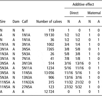
Individual heterozygosity (IH) was calculated according to Teixeira and Albuquerque (Reference Teixeira and Albuquerque2003) as follows: IH = sire breed + dam breed − 2 × (sire breed × dam breed), where breed = Zebu fraction of the individual. Maternal heterozygosity was not considered as only purebred Nelore or Angus cows were used as dams (Table 1).
Composition of the genetic groups and definition of direct and maternal additive effects in cattle forming the Brangus breed

N = Nelore; A = Angus.
Values in the genetic groups correspond to the portion of each breed in the composition of the groups, for example, 1N3A = 1/4 Nelore + 3/4 Angus.
The contemporary group at weaning consisted of animals of the same sex born on the same farm in the same season and year, and scored on the same day, farm and management group at weaning. At yearling, the same contemporary group as that used at weaning was defined, including the day, farm and management group at yearling. Contemporary groups containing fewer than five animals were eliminated. Dam age at calving ranged from 2 to 15 years, whereas the variable season of birth was divided into four periods of 3 months each, starting in January.
Statistical analysis
The (co)variance components of the variables studied were estimated by the derivative-free maximum likelihood method in single- and two-trait analyses using the MTDFREML program (Boldman et al., Reference Boldman, Kreise, Van Vleck, VanTassel and Kachaman1995). The general model that was proposed included the contemporary group and the covariate age of dam in years (linear and quadratic effects), age of animal at weaning (linear and quadratic effects), age of animal at yearling (linear effect), in days, and IH (linear effect) as fixed effects, and direct and maternal additive genetic effects and maternal permanent environmental effects as random effects.
The single-trait animal model used can be represented as

where y is a n × 1 vector of records, β denotes the vector of fixed effects, X is a matrix that associates β with y, g is a vector of random additive direct genetic effects, Z is a matrix that associates g with y, m is a vector of random maternal additive genetic effects, M is a matrix that associates m with y, p is a vector of random effects of maternal permanent environment plus non-additive genetic effects contributed by dams to records of their progeny, W is a matrix that associates p with y, and e is the vector of random residual effects, peculiar to observations, that are not explained by other parts of the model. Assumptions for this model are:


The multiple-trait animal model can be represented as

where the subscripts 1 and 2 represent traits 1 and 2, respectively. As before, assumptions for this model are:

The co(variance) matrix for genetic effects is G = G 0⊗A, where

and ⊗ denotes the direct product operator.
As shown in G 0, the direct genetic effect for one trait was assumed to be uncorrelated to the genetic maternal effect for the other trait. The (co)variance matrix for permanent environmental effects is P = P 0⊗I c, where 
The residual (co)variance of random residual effects was assumed to be R = R 0⊗I n, where 
In both models, c is the number of cows, n is the number of observations, A is the numerator relationship matrix, I are identity matrices of appropriate order. For the i th trait,  denotes the additive genetic variance,
 is the maternal additive genetic variance, σgmi is the covariance between direct and maternal additive effects,
 is the permanent environmental variance and
 is the residual variance.
Non-zero covariance between traits 1 and 2 was considered for direct additive (σg 12), maternal additive (σm 12), maternal permanent environment (σp 12) and residual (σe 12) random effects. For both models, covariance between direct or maternal effects and any of the remainder effects (i.e. p and e) was assumed to be zero, as well as the covariance between the random effects p and e.
A likelihood ratio test was used to compare the preweaning models and to evaluate the significance of maternal genetic random effects. As the latter effect was found to be non-significant (P > 0.01) for CW, PW and MW scores, it was not included in the models for these scores, but was included in the model for GBW. For yearling traits, maternal genetic and permanent environmental effects were also not included as they were not found to be important after weaning. The effect of age of dam at calving was taken as linear in the models for CY, PY and MY scores as the quadratic effect was not significant (P > 0.05) in a previous analysis using the GLM procedure of the SAS 9.1 program (SAS Institute Inc., Cary, NC, USA).
Single-trait analyses were first performed for all the traits that were studied. The variance components obtained with these analyses were used as initial values for the two-trait analyses. Genetic covariance between direct and maternal additive effects was set to zero (Muniz et al., Reference Muniz, Carvalheiro, Fries and Queiroz2005).
Results and discussion
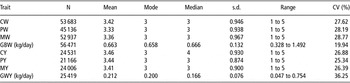
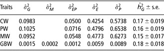
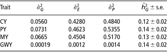
Table 2 shows the descriptive statistics of the traits studied. The estimates of variance components and direct additive heritability for weaning and yearling traits obtained with the single-trait models are shown in Tables 3 and 4. Similar direct heritability estimates of 0.17 ± 0.02, 0.16 ± 0.02, 0.15 ± 0.02 and 0.18 ± 0.02 were obtained for CW, PW and MW scores and GBW, respectively. For further details regarding these results see Costa et al. (Reference Costa, Queiroz, Oliveira and Fries2008). The same pattern was observed for the heritability estimates of yearling traits (Table 4).
Descriptive statistics of weaning and yearling visual scores and weight gain in cattle forming the Brangus breed

CW = conformation at weaning; PW = precocity at weaning; MW = muscling at weaning; GBW = average daily gain from birth to weaning; CY = conformation at yearling; PY = precocity at yearling; MY = muscling at yearling; GWY = average daily gain from weaning to yearling.
Estimates of variance components and heritability obtained by single-trait analysis for weaning visual scores and weight gain in cattle forming the Brangus breed

 = direct additive genetic variance;
 = direct additive maternal variance;
 = permanent maternal environment variance;
 = residual variance;
 = phenotypic variance;
 = direct additive heritability; CW = conformation at weaning; PW = precocity at weaning; MW = muscling at weaning; GBW = average daily gain from birth to weaning.
Estimates of variance components and heritability obtained by single-trait analysis for yearling visual scores and weight gain in cattle forming the Brangus breed

 = direct additive genetic variance;
 = residual variance;
 = phenotypic variance;
 = direct additive heritability; CY = conformation at yearling; PY = precocity at yearling; MY = muscling at yearling; GWY = average daily gain from weaning to yearling.
The heritability estimates for yearling visual scores and GWY were lower than those observed for the weaning traits, suggesting that phenotypic selection for either weaning or yearling traits would result in a small response in the herds studied (Tables 3 and 4). The low estimates obtained were probably due to large variations in the environment to which the animals were exposed as they belonged to herds from three different regions of Brazil. It is possible that the models used were unable to completely remove all environmental variation.
The heritabilities for yearling traits found in this study (Table 4) were lower than those reported for the same traits by Cardoso et al. (Reference Cardoso, Cardellino and Campos2004), who estimated values of 0.19, 0.25, 0.26 and 0.20 for CY, PY, MY and GWY, respectively, in Angus animals, and by Faria et al. (Reference Faria, Magnabosco, Albuquerque, Bezerra and Lôbo2009) for the visual evaluation of M in Nelore cattle at 15 and 22 months of age. Using Bayesian analysis, Faria et al. (Reference Faria, Magnabosco, Albuquerque, Bezerra and Lôbo2009) obtained mean heritability estimates of 0.38 and 0.21 for M at these two ages. In addition, mean estimates obtained for C at the same ages were 0.07 and 0.29, respectively. Pons et al. (Reference Pons, Milagres and Regazzi1990a) reported a heritability of 0.34 for C. In two different studies involving Nelore animals, Eler et al. (Reference Eler, Ferraz and Silva1996a and Reference Eler, Ferraz and Silva1996b) obtained heritability estimates ranging from 0.23 to 0.34 for postweaning C, P and M scores. The differences in heritability estimates for yearling visual scores between this study and the literature might be attributed to variations between observers, to genetic differences between populations, or even to differences in the visual evaluation system. Visual evaluation using scores varies among breeding programs. Scores might be attributed by one observer in one program and by three observes in another. In the latter case, the animal is scored by consensus among observers. A score ranging from 1 to 6 has been reported in some programs, whereas most programs report scores ranging from 1 to 5.
Higher heritabilities for average postweaning gain than those observed in this study have been reported by other investigators. In this respect, Koots et al. (Reference Koots, Gibson and Wilton1994) reported average heritability of 0.40 for postweaning weight gain of beef cattle. Kriese et al. (Reference Kriese, Bertrand and Benyshek1991) obtained estimates of 0.31 and 0.15 for weight gain of Brahman and Brangus cattle from weaning to 365 days of age, respectively.
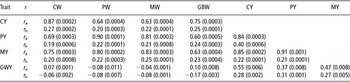
Table 5 shows the genetic and environmental correlation estimates between weaning and yearling traits obtained by two-trait analysis. Maternal effects were included in the model for GBW and maternal permanent environmental effects were only included in the models for weaning traits.
Estimates of genetic (r a) and environmental (r e) correlations (respective s.e.) between weaning and yearling visual scores and weight gain obtained by two-trait analysis for cattle forming the Brangus breed

CW = conformation at weaning; PW = precocity at weaning; MW = muscling at weaning; GBW = average daily gain from birth to weaning; CY = conformation at yearling; PY = precocity at yearling; MY = muscling at yearling; GWY = average daily gain from weaning to yearling.
The estimated genetic correlations between the same visual scores obtained at weaning and yearling, for example, CW v. CY, were very strong (>0.83; Table 5). In the literature, this association was only reported by Cardoso et al. (Reference Cardoso, Cardellino and Campos2004), who obtained correlations between scores stronger than 0.90 in the Angus animals. Correlation estimates between the different scores obtained at weaning and yearling were also strong (>0.63; Table 5). We found no reports of such correlations in the literature.
The genetic correlation between pre- and postweaning average daily gains estimated in this study was 0.10 ± 0.008 (Table 5). This result suggests that the genes involved in preweaning growth are not the same or are not expressed during the yearling period, indicating that most genes responsible for the expression of GBW do not continue acting on the expression of GWY. Thus, animals that gain more weight from birth to weaning may not be the same as those that will gain more weight after weaning. However, although the estimated value indicates a very weak association between the two traits, it contradicts results from previous studies. In a review on genetic parameters of productive traits in beef cattle, Koots et al. (Reference Koots, Gibson and Wilton1994) found a mean genetic correlation of 0.39 between pre- and postweaning gains. In a recent study of growth in beef cattle to detect SNP associations with body weight and weight gain at different ages, Snelling et al. (Reference Snelling, Allan, Keele, Kuehn, McDaneld, Smith, Sonstergard, Thallman and Bennett2010) also demonstrated that most of the SNPs showing highly significant associations between genotype and growth phenotypes coincided with previously described quantitative trait loci for growth or correlated traits. The estimated correlation might be explained in part by compensatory gain during the postweaning period, that is, animals born to younger or older cows, which showed poorer growth during the preweaning period, presented accelerated growth after the cessation of feed restriction, reducing the intensity of the genetic association between these traits. The model possibly did not account efficiently for the environmental effects even when maternal permanent environmental effects and age of cow at calving were included. This hypothesis is supported by the environmental correlation estimate between GBW and GWY (−0.17 ± 0.016; Table 5), indicating weak antagonism between environmental and non-additive genetic effects that act on the two traits. However, this result agrees with Cardoso et al. (Reference Cardoso, Cardellino and Campos2004), Marcondes et al. (Reference Marcondes, Bergmann, Eler, Ferraz, Pereira and Penna2000) and Sarmento et al. (Reference Sarmento, Pimenta Filho, Ribeiro and Martins Filho2003) who reported genetic correlation estimates of 0.23, 0.23 and 0.22, respectively, between pre- and postweaning weight gains.
GBW showed a strong positive genetic correlation with the visual scores of CY, PY and MY (0.75, 0.60 and 0.63, respectively). These correlations suggest that animals with good preweaning body development presented higher yearling scores because they had already achieved a better degree of performance than those presenting poorer GBW.
Very weak genetic correlations (basically zero) were observed between the visual scores evaluated at weaning and GWY indicating that selection for weaning visual scores will not influence postweaning gain.
Yearling visual scores were positively associated with genetic correlations higher than 0.84. However, these correlations were slightly weaker than those observed at weaning according to the results reported by Costa et al. (Reference Costa, Queiroz, Oliveira and Fries2008) for the same data. Similar to the weaning results, the magnitude of these correlations might be attributed to differences in the evaluation system. Pons et al. (Reference Pons, Polastre and Cardellino1990b), studying Hereford animals at postweaning, estimated lower genetic correlations between the same scores ranging from 0.30 to 0.68. Eler et al. (Reference Eler, Ferraz and Silva1996b) obtained a genetic correlation of 0.86 between CY and PY, of 0.82 between CY and MY, and of 0.96 between PY and MY for Nelore animals. Similar results have been reported by Cardoso et al. (Reference Cardoso, Cardellino and Campos2004) for Angus cattle.
The genetic correlations between yearling visual scores and GWY were of medium magnitude and ranged from 0.37 to 0.55. The lowest correlation was observed between PY and GWY (0.37). This result might be explained by the fact that a higher GWY indicates faster weight gain irrespective of the biotype of the animal. However, animals presenting greater weight gain, lower rib depth and no carcass finishing receive lower PY scores. Similar genetic correlations have been reported by Koury Filho (Reference Koury Filho2001) for Nelore animals. In contrast, Cardoso et al. (Reference Cardoso, Cardellino and Campos2004) estimated higher correlations for Angus cattle.
Environmental correlations between the traits (Table 5) ranged from −0.17 (GWY v. GBW) to 0.40 (PY v. CY). These estimates indicate a weak association between environmental effects for all traits and revealed that the environmental conditions provided for animals from birth to weaning are almost independent of those at yearling.
Conclusions
Visual scores for conformation, early finishing (precocity) and muscling at weaning and yearling might be included as selection criteria in the breeding program of the Brangus breed in Brazil in order to help producers meet industry expectations, although selection based on these traits will not result in large genetic changes in these traits. In addition, selection for weaning visual scores would have a marked effect on yearling visual scores, and selection for average daily gain during the preweaning period would result in a correlated genetic response in visual scores during life.
Acknowledgement
The authors are thankful to Gensys consultants associates LTDA for providing the data used in this research.