1.1 The importance of helicity segregation for dynamo action

Plausible cartoons of a mean-field geodynamo have been around for the better part of half a century (Parker Reference Parker1955, Steenbeck, Krause & Radler Reference Steenbeck, Krause and Radler1966, Moffatt Reference Moffatt1978). Moreover, over the last decade or so, the numerical simulations of planetary dynamos have increasingly acquired Earth-like features, such as a dipolar field aligned with the rotation axis, the westward drift of flux patches and occasional reversals (Christensen & Wicht Reference Christensen, Wicht and Olson2007, Jones Reference Jones2011). Admittedly, these simulations are a long way from any geophysical regime, being overly viscous by a factor of $10^{8}\rightarrow 10^{9}$ , as measured by the Ekman number, $Ek=\unicode[STIX]{x1D708}/\unicode[STIX]{x1D6FA}R_{C}^{2}$ , and they under-rotate by a factor of ${\sim}10^{3}$ , as measured by the Rossby number, $Ro=|\boldsymbol{u}|/\unicode[STIX]{x1D6FA}R_{C}$ (see Christensen Reference Christensen2011), where $\unicode[STIX]{x1D708}$ is the kinematic viscosity, $\unicode[STIX]{x1D6FA}$ the planetary rotation rate and $R_{C}$ the radius of the conducting core. They are also thought to be significantly underpowered, perhaps by a factor of approximately $10^{2}\rightarrow 10^{3}$ , as measured by the ratio of the buoyancy flux to the flux at which convection first sets in (Gubbins Reference Gubbins2001, Christensen & Aubert Reference Christensen and Aubert2006, Christensen Reference Christensen2011). Despite this, many of the more recent simulations seem to yield plausible looking dynamos. So, despite the fact that the simulations must contain many features which are fundamentally inconsistent with a geophysical dynamo, it is probable that they realise certain processes which are geophysically relevant. Of course, if we wish to extrapolate the results of the simulations to the planets, it is crucial that we can distinguish between those processes which are artefacts of the unphysical parameter regime and those which are transferable to a planet. Unfortunately, there is little agreement on this point.

Figure 1.

Typical flow structure in the numerical dynamos: (a) the radial velocity near the core mantle boundary shows columnar vortices which appear in cyclone, anticyclone pairs; (b) the azimuthally averaged helicity outside the tangent cylinder is negative in the north and positive in the south. (From Ranjan et al. Reference Ranjan, Davidson, Christensen and Wicht2018.)

Nevertheless, a cartoon for planetary dynamo action has emerged from these simulations which has gained some traction. While there can be powerful upwellings within the tangent cylinder which drive a local $\unicode[STIX]{x1D6FA}$ -effect (Schaeffer et al. Reference Schaeffer, Jault, Nataf and Fournier2017), typically the dynamo action resides outside the tangent cylinder. Here the $\unicode[STIX]{x1D6FA}$ -effect is weak and the flow is dominated by columnar vortices aligned with the rotation axis, often in the form of alternating cyclones and anticyclones arranged around the solid inner core (figure 1 a). These columnar vortices are observed to be highly helical, with the helicity outside the tangent cylinder, $h=\boldsymbol{u}\boldsymbol{\cdot }\unicode[STIX]{x1D735}\times \boldsymbol{u}$ , predominantly negative in the north and positive in the south (figure 1 b). Of course, just such an antisymmetric helicity distribution is exactly what is required for a quasi-steady, dipolar, $\unicode[STIX]{x1D6FC}^{2}$ dynamo (Moffatt Reference Moffatt1978). In summary, then, the zero-order cartoon that emerges from these numerical experiments is one of an $\unicode[STIX]{x1D6FC}^{2}$ dynamo located outside the tangent cylinder and driven by helical motion in the columnar convection cells (Olson, Christensen & Glatzmaier Reference Olson, Christensen and Glatzmaier1999, Christensen Reference Christensen2011, Jones Reference Jones2011).

So the phenomenological basis for most of these numerical dynamos is Parker’s lift-and-twist mechanism (Parker Reference Parker1955), as shown in figure 2(a). This drives an $\unicode[STIX]{x1D6FC}$ -effect, as formalised by Steenbeck et al. (Reference Steenbeck, Krause and Radler1966), in which the induced e.m.f. tends to be parallel or anti-parallel to the ambient magnetic field $\boldsymbol{B}$ , depending on the sign of the helicity (Moffatt Reference Moffatt1978). That is, helical disturbances with positive helicity tend to generate an e.m.f. which is anti-parallel to $\boldsymbol{B}$ as shown schematically in figure 2(b), while disturbances with negative helicity tend to generate an e.m.f. which is parallel to $\boldsymbol{B}$ . Of course, the formalism of mean-field electrodynamics as applied to planetary cores is often questioned, as there is possibly no clear separation of scales. However, at a phenomenological level, mean-field electrodynamics is still a useful way to categorise the results of the numerical simulations, and to capture the various dynamo mechanisms, if only in a cartoon-like fashion.

Figure 2.

(a) One of Parker’s helical disturbances lifts and twists the east–west magnetic field lines. (Adapted from Cowling Reference Cowling1957.) (b) Helical disturbances with positive helicity tend to generate an e.m.f. which is anti-parallel to $\boldsymbol{B}$ . Conversely, helical disturbances with negative helicity tend to generate an e.m.f. which is parallel to $\boldsymbol{B}$ .

This type of mean-field $\unicode[STIX]{x1D6FC}^{2}$ dynamo cycle is shown schematically in figure 3, where we have chosen the signs of $h$ in the north and the south to be the same as those observed outside the tangent cylinder in figure 1. Here we use cylindrical polar coordinates $(r,\unicode[STIX]{x1D703},z)$ , $\boldsymbol{B}_{p}$ and $\boldsymbol{B}_{\unicode[STIX]{x1D703}}$ are the poloidal and azimuthal components of the azimuthally averaged magnetic field, $\boldsymbol{J}_{p}$ is the poloidal current density induced by the $\unicode[STIX]{x1D6FC}$ -effect operating on the radial magnetic field and $\boldsymbol{J}_{\unicode[STIX]{x1D703}}$ is the azimuthal current driven by the $\unicode[STIX]{x1D6FC}$ -effect operating on the azimuthal magnetic field. To get a self-consistent dipolar dynamo with helicity antisymmetric about the equator, $\boldsymbol{B}_{\unicode[STIX]{x1D703}}$ must also be antisymmetric about the equator. In particular, with negative helicity in the north and positive helicity in the south, we require a mean azimuthal field outside the tangent cylinder which is positive in the north and negative in the south, which is precisely what is observed in most numerical dynamos.

Figure 3.

An $\unicode[STIX]{x1D6FC}^{2}$ dynamo driven by helicity whose sign is antisymmetric about the equator. The dipole points to the north.

Of course, if we are to extend this dynamo cartoon to the planets, we must identify what drives the helical flow in the convection cells. Moreover, we need to explain why there is a spatial segregation of helicity, with $h$ predominantly negative in the north and positive in the south. In this respect it is important to remember that the Earth is a rapid rotator, in the sense that the Rossby number is small, around $Ro=|\boldsymbol{u}|/\unicode[STIX]{x1D6FA}R_{C}\sim 10^{-6}$ . So the core of the Earth is a wave-bearing system, almost certainly awash with helical waves. These may be both inertial waves and combined magnetic-Coriolis waves, such as magnetostrophic waves. While $Ro$ in the simulations is much larger than that in the Earth, the numerical dynamos also operate in the low- $Ro$ regime.

1.2 The absence of an agreed mechanism of helicity segregation

One of the main stumbling blocks to extrapolating the results of the simulations to the planets is the absence of an agreed mechanism for the north–south helicity segregation, either within planetary cores or in the numerical dynamos. In the early numerical simulations, which were excessively viscous and only mildly supercritical, the helicity distribution was sometimes attributed, at least in part, to viscous Ekman pumping driven by the interaction of the convection columns with the mantle (Kono, Sakuraba & Ishida Reference Kono, Sakuraba and Ishida2000, Roberts & King Reference Roberts and King2013). In such a cartoon, the columnar vortices are seen as quasi-steady structures that span the core and grind away on the mantle, inducing helical Ekman pumping. Certainly, such Ekman pumping can produce the required asymmetric distribution of helicity, i.e. negative in the north and positive in the south (Davidson Reference Davidson2014). However, while it is clear that columnar vortices can stretch from mantle to mantle in mildly supercritical dynamo simulations, from which this dynamo cartoon has emerged, the more recent numerical simulations tend to be much more supercritical and here the columnar vortices are often interior objects, in the sense that they do not span the core, and so do not interact strongly with the mantle (Ranjan et al. Reference Ranjan, Davidson, Christensen and Wicht2018). Given that the degree of supercriticality in the Earth is thought to be two orders of magnitude larger than that in even the most strongly driven numerical dynamos, this becomes a major consideration when trying to extend this viscous mechanism to the planets. (Incidentally, this also suggests that Rossby waves, which require quasi-geostrophic vortices to span the core, are also not an efficient mechanism for generating helicity.) Moreover, even in those simulations for which the forcing is modest, it has long been recognised that some of the helicity comes not from the boundary, but from the interior, originating from inhomogeneities in density (Olson et al. Reference Olson, Christensen and Glatzmaier1999). It seems probable that, as the degree of supercriticality increases in the simulations, this supplementary source of helicity progressively displaces Ekman pumping as the primary mechanism of helicity generation. Finally, and most importantly, we note that those numerical simulations in which a free-slip condition is used at the core mantle boundary still yield dipolar dynamos (see, for example, Yadav, Gastine & Christensen Reference Yadav, Gastine and Christensen2013), and Ekman pumping cannot supply the helicity in such cases. In short, Ekman pumping cannot explain the success of the numerical dynamos.

It is also extremely unlikely that the helicity in a planet could be generated by viscous boundary layers on the mantle. There are at least two reasons for believing this. First, even if we believed that the columnar vortices spanned the core of the Earth, viscous scaling theory requires an Ekman layer thickness of $\unicode[STIX]{x1D6FF}_{E}\sim (Ek)^{1/2}R_{C}$ , and the estimated Ekman number of $Ek\sim 10^{-15}$ for the Earth then demands a boundary layer thickness of approximately 10 cm and a convection column width, $\unicode[STIX]{x1D6FF}\sim (Ek)^{1/3}R_{C}$ , of a few tens of metres. Such tiny values seem inconceivable in the core.

Second, the observed properties of the dynamos operating in the gas giants look surprisingly similar to those in the terrestrial planets, being predominantly dipolar and with the magnetic axis roughly aligned with the rotation axis. Moreover, the normalised magnetic field strength is remarkably consistent across the planets. That is to say, the three observable properties of the planetary dynamos are the planetary rotation rate, $\unicode[STIX]{x1D6FA}$ , the planet size, from which we can infer a conducting core size, $R_{C}$ , and the dipole moment, $\boldsymbol{m}$ , from which we may determine the mean axial field strength in the core of the planet,

(1.1) $$\begin{eqnarray}\displaystyle & \displaystyle \bar{B}_{z}=\frac{2\unicode[STIX]{x1D707}}{3V_{C}}|\boldsymbol{m}|. & \displaystyle\end{eqnarray}$$

(Here $V_{C}$ is the volume of the conducting core and $\unicode[STIX]{x1D707}$ the permeability of free space.) From these three parameters we can construct the dimensionless field strength

(1.2) $$\begin{eqnarray}\displaystyle & \displaystyle \unicode[STIX]{x1D6F1}_{B}={\displaystyle \frac{\bar{B}_{z}/\sqrt{\unicode[STIX]{x1D70C}\unicode[STIX]{x1D707}}}{\unicode[STIX]{x1D6FA}R_{C}}}, & \displaystyle\end{eqnarray}$$

where $\unicode[STIX]{x1D70C}$ is density. (This is sometimes called the Lehnert number.) The estimated values of this dimensionless field strength are given in table 1 for the various planets, as well as for the fully convective, M-dwarf star V374 Pegasi, whose properties have been well studied and which is thought to exhibit an $\unicode[STIX]{x1D6FC}^{2}$ dipolar field. The various estimates of $\unicode[STIX]{x1D6F1}_{B}$ are remarkably consistent across the planets, and indeed for the M-dwarf star. It seems plausible, therefore, that the underlying structure of the dynamos operating in the gas giants is not dissimilar to that in the Earth, yet there is no mantle in the gas giants on which Ekman layers can form. So Occam’s razor suggests that we set aside viscous Ekman pumping as a mechanism for helicity segregation in the planets.

Figure 4.

Approximate structure of the planets. (Figure courtesy of Uli Christensen.)

Table 1.

Approximate properties of the planets and their magnetic fields. V374 Pegasi, which is a fully convective, M-dwarf star, is shown for comparison. (From Davidson Reference Davidson2016.)

It is striking that the normalised field strengths, $\unicode[STIX]{x1D6F1}_{B}$ , observed in these very different astrophysical objects is so uniform, despite their different internal structures, sizes and rotation rates (figure 4). By contrast, the Elsasser number,

(1.3) $$\begin{eqnarray}\displaystyle & \displaystyle \unicode[STIX]{x1D6EC}={\displaystyle \frac{\unicode[STIX]{x1D70E}\bar{B}_{z}^{2}}{\unicode[STIX]{x1D70C}\unicode[STIX]{x1D6FA}}}=\unicode[STIX]{x1D6F1}_{B}^{2}{\displaystyle \frac{\unicode[STIX]{x1D6FA}R_{C}^{2}}{\unicode[STIX]{x1D706}}}, & \displaystyle\end{eqnarray}$$

which is often assumed to adopt a value of order unity in planetary dynamos, varies by eight orders of magnitude in table 1. (Here $\unicode[STIX]{x1D70E}$ is the electrical conductivity and $\unicode[STIX]{x1D706}=1/\unicode[STIX]{x1D70E}\unicode[STIX]{x1D707}$ the magnetic diffusivity.) The usual rationalisation of $\unicode[STIX]{x1D6EC}\sim 1$ is that the Lorentz force, which is taken to be of order $|\boldsymbol{J}\times \boldsymbol{B}|\sim \unicode[STIX]{x1D70E}uB^{2}$ , is of the same order of magnitude as the Coriolis force, $2\unicode[STIX]{x1D70C}\boldsymbol{u}\times \unicode[STIX]{x1D734}$ . However this is too simplistic, as the flow in the core of the Earth is almost certainly strongly anisotropic, being highly elongated along the rotation axis. This is important because the curl and divergence of the Coriolis force are

(1.4a,b ) $$\begin{eqnarray}\displaystyle & \displaystyle \unicode[STIX]{x1D735}\times (\boldsymbol{u}\times \unicode[STIX]{x1D734})=(\unicode[STIX]{x1D734}\boldsymbol{\cdot }\unicode[STIX]{x1D735})\boldsymbol{u},\quad \unicode[STIX]{x1D735}\boldsymbol{\cdot }(\boldsymbol{u}\times \unicode[STIX]{x1D734})=\unicode[STIX]{x1D734}\boldsymbol{\cdot }\unicode[STIX]{x1D735}\times \boldsymbol{u}. & \displaystyle\end{eqnarray}$$

So when the flow is strongly anisotropic, the curl of the Coriolis force is much smaller than its divergence. Consequently, if we perform a Helmholtz decomposition on the Coriolis force, dividing it into irrotational and solenoidal-rotational parts, the dominant term is the former. Of course, the irrotational part of the Coriolis force is simply balanced by pressure gradients and so the Lorentz force, if order one, should be balanced against the much weaker rotational component. This then removes the usual justification of the estimate $\unicode[STIX]{x1D6EC}\sim 1$ (Davidson Reference Davidson2013b , Reference Davidson2017), consistent with table 1.

In summary, if we want to extrapolate the dynamo cartoon that has emerged from the numerical simulations to the planets, we are obliged to identify a source of helicity which operates in both planetary cores and numerical dynamos. This should be robust, independent of viscosity and not reliant on the presence of a mantle. Moreover, this source must yield a helicity distribution which is negative in the north and positive in the south, in accordance with the simulations.

In this review we explore the possibility that helical waves, particularly inertial waves, provide this asymmetric distribution of helicity. Of course, the idea that helical waves could be an important ingredient in dynamo action is not new (Moffatt Reference Moffatt1970, Moffatt Reference Moffatt1978, Olson Reference Olson1981). However, only recently has such a self-consistent dynamo cartoon been proposed and its dynamical consequences explored in detail. In particular, we examine the recent suggestion that these waves are driven by the observed equatorial bias in the buoyancy flux in the outer core (Davidson Reference Davidson2014, Davidson & Ranjan Reference Davidson and Ranjan2015), as illustrated in figure 5. Such a bias is seen in, for example, Olson et al. (Reference Olson, Christensen and Glatzmaier1999), Sakuraba & Roberts (Reference Sakuraba and Roberts2009), Sheyko (Reference Sheyko2014), Schaeffer et al. (Reference Schaeffer, Jault, Nataf and Fournier2017) and Ranjan et al. (Reference Ranjan, Davidson, Christensen and Wicht2018).

The structure of the paper is as follows. In § 2 we remind readers that inertial waves are the very mechanism by which columnar vortices first form and subsequently evolve. Next, in § 3, we show that inertial waves triggered by the equatorial bias in the buoyancy flux produce the required helicity distribution outside the tangent cylinder, being negative in the north and positive in the south, and in § 4, we estimate the mean-field e.m.f. induced by such axially propagating inertial wave packets, comparing this e.m.f. against numerical simulations. Finally, in § 5, we derive scaling laws for this kind of helical-wave planetary dynamo. We then compare these predictions with the numerical dynamos and also with what little we know about the planets.

Figure 5.

(a) The azimuthally averaged radial velocity in one of the simulations of Sakuraba & Roberts (Reference Sakuraba and Roberts2009). (b) The root-mean-square (r.m.s.) azimuthal temperature gradient, averaged in the azimuth, in the simulation of Ranjan et al. (Reference Ranjan, Davidson, Christensen and Wicht2018). (c) The distribution of relative helicity, $h/|\boldsymbol{u}||\unicode[STIX]{x1D74E}|$ , in a simulation by Schaeffer et al. (Reference Schaeffer, Jault, Nataf and Fournier2017).

Our central thesis is that the spontaneous generation of helical waves in the outer core is not just some incidental artefact of columnar convection, but rather is the fundamental mechanism by which quasi-geostrophic motion is maintained in a forced turbulent system. To that end, we start by reminding the reader of the well-documented properties of rapidly rotating turbulence, which is inevitably dominated by long-lived, helical, columnar vortices.

2.1 The evidence from laboratory experiments and numerical simulations of turbulence

Laboratory and numerical experiments tell us that rapidly rotating turbulence which is subject to some form of random forcing, or else is unforced but emerges from random initial conditions, is inevitably dominated by vortices which are axially elongated in the direction of the rotation axis. This occurs in both laboratory experiments (Ibbetson & Tritton Reference Ibbetson and Tritton1975, Dickenson & Long Reference Dickenson and Long1983, Staplehurst, Davidson & Dalziel Reference Staplehurst, Davidson and Dalziel2008), and in numerical simulations (Thiele & Muller Reference Thiele and Muller2009, Pouquet & Mininni Reference Pouquet and Mininni2012, Ranjan & Davidson Reference Ranjan and Davidson2014). The energy source may be mechanical in nature (Wigeland & Nagib Reference Wigeland and Nagib1978, Hopfinger, Browand & Gagne Reference Hopfinger, Browand and Gagne1982), due to buoyant anomalies in a Boussinesq fluid (Davidson Reference Davidson2014, Davidson & Ranjan Reference Davidson and Ranjan2015), or just random initial conditions (Morize, Moisy & Rabaud Reference Morize, Moisy and Rabaud2005, Davidson, Staplehurst & Dalziel Reference Davidson, Staplehurst and Dalziel2006, Morize & Moisy Reference Morize and Moisy2006). In all three of these cases, the large scales of the turbulence turns out to be dominated by long-lived columnar vortices. These vortices are dynamic in nature, in the sense that they evolve rapidly in time, and are typically helical. Crucially, in all of the studies cited above, the boundaries play no role in establishing the columnar vortices, the only exception being Ibbetson & Tritton (Reference Ibbetson and Tritton1975) at late times. It follows that Rossby waves, for example, play no important role in the dynamics here.

Both laboratory experiments and numerical simulations indicate that the appearance of these columnar vortices occurs whenever the Rossby number based on the integral scales of the turbulence, $Ro=u/\unicode[STIX]{x1D6FA}\ell$ , is less than approximately $Ro\sim 0.4$ , the precise value depending on exactly how the integral scales, $u$ and $\ell$ , are defined (Staplehurst et al. Reference Staplehurst, Davidson and Dalziel2008, Bin Baqui & Davidson Reference Bin Baqui and Davidson2015). Perhaps not surprisingly, this regime turns out to correspond to that in which inertial waves can propagate through the fluid. That is to say, it is observed that inertial waves can propagate in a quasi-linear manner through a still fluid (still in the rotating frame) whenever $Ro$ is less than $0.4\rightarrow 1$ , but nonlinear effects become very evident in the range $1\rightarrow 2$ and indeed no waves are observed whenever $Ro$ exceeds a value of around $2\rightarrow 3$ (Maxworthy Reference Maxworthy1970, Wang, Lu & Zhuang Reference Wang, Lu and Zhuang2004, Sreenivasan & Davidson Reference Sreenivasan and Davidson2008). Of course, the exact value of $Ro=u/\unicode[STIX]{x1D6FA}\ell$ at which waves cease to propagate depends on the precise definitions of $u$ and $\ell$ .

Typical examples of rapidly rotating turbulence are shown in figures 6 and 7, both being numerical simulations in a periodic domain. Figure 6 is from Davidson (Reference Davidson2013a ) and shows freely decaying, rapidly rotating turbulence at $Ro\sim 0.1$ , visualised by helicity, while figure 7 is from Pouquet & Mininni (Reference Pouquet and Mininni2012), and shows forced turbulence at $Ro\sim 0.06$ , visualised by vorticity. Columnar eddies are evident in both cases. In figure 6 the initial condition consists of randomly orientated vortices distributed in and around the central plane of the computational domain. Notice that, at $\unicode[STIX]{x1D6FA}t=6$ , the flow in the upper half of the domain has a helicity that is uniformly negative, while that in the lower half has positive helicity. Although the energy source here is the kinetic energy of the initial eddies, essentially the same pattern is obtained in a Boussinesq fluid if buoyant anomalies are distributed near the central plane (Davidson & Ranjan Reference Davidson and Ranjan2015).

Figure 6.

Numerical simulation of freely decaying, rapidly rotating turbulence at $Ro\sim 0.1$ , visualised by helicity. The initial condition is on the left and the flow at $\unicode[STIX]{x1D6FA}t=6$ is on the right. Red marks negative helicity and green positive helicity. (From Davidson Reference Davidson2013a .)

Figure 7.

Numerical simulation of forced, rapidly rotating turbulence at $Ro\sim 0.06$ , visualised by vorticity. See Pouquet & Mininni (Reference Pouquet and Mininni2012), for a full description of the figure.

In the turbulence literature, it is often argued that columnar vortices in rotating turbulence form slowly on a time scale of 1/ $Ro$ through weakly nonlinear interactions; so-called resonant triad interactions. However, this is clearly not the case in figure 6, as there is insufficient time for weak nonlinearities to play any significant role. In fact, as we shall see, the columnar structures on the right of figure 6 are simply inertial wave packets propagating along the rotation axis. Indeed, this is almost evident from the spatial segregation of helicity shown on the right of figure 6, since upward propagating inertial waves carry negative helicity, while downward propagating waves carry positive helicity. (The properties of monochromatic inertial waves are outlined in the Appendix.) Such wave packets will turn out to be of crucial importance in the numerical simulation of planetary cores.

2.2 The Taylor–Proudman theorem revisited

The appearance of columnar vortices in a rapidly rotating system is often attributed to the Taylor–Proudman theorem, but this can be misleading and has led to some confusion. To see why, let us recall what the theorem says. In a rotating frame of reference the inviscid equation of motion is,

(2.1) $$\begin{eqnarray}\displaystyle & \displaystyle {\displaystyle \frac{\text{D}\boldsymbol{u}}{\text{D}t}}=2\boldsymbol{u}\times \unicode[STIX]{x1D734}-\unicode[STIX]{x1D735}(p/\unicode[STIX]{x1D70C}), & \displaystyle\end{eqnarray}$$

where $\unicode[STIX]{x1D734}=\unicode[STIX]{x1D6FA}\hat{\boldsymbol{e}}_{z}$ is the background rotation. We are particularly interested in cases where the Rossby number is small and so the inertial term $\boldsymbol{u}\boldsymbol{\cdot }\unicode[STIX]{x1D735}\boldsymbol{u}$ may be neglected by comparison with the Coriolis force. Dropping $\boldsymbol{u}\boldsymbol{\cdot }\unicode[STIX]{x1D735}\boldsymbol{u}$ and taking the curl of (2.1) yields the linearised vorticity equation,

(2.2) $$\begin{eqnarray}\displaystyle & \displaystyle {\displaystyle \frac{\unicode[STIX]{x2202}\unicode[STIX]{x1D74E}}{\unicode[STIX]{x2202}t}}=2(\unicode[STIX]{x1D734}\boldsymbol{\cdot }\unicode[STIX]{x1D735})\boldsymbol{u}. & \displaystyle\end{eqnarray}$$

If the motion is quasi-steady we might neglect $\unicode[STIX]{x2202}\unicode[STIX]{x1D74E}/\unicode[STIX]{x2202}t$ , which yields $(\unicode[STIX]{x1D734}\boldsymbol{\cdot }\unicode[STIX]{x1D735})\boldsymbol{u}=0$ . We have arrived at the Taylor–Proudman theorem: in cases where $u\ll \unicode[STIX]{x1D6FA}\ell$ and $\unicode[STIX]{x2202}\boldsymbol{u}/\unicode[STIX]{x2202}t$ is negligible, the motion must be two-dimensional, in the sense that $\boldsymbol{u}$ is not a function of $z$ .

Figure 8.

The effect of moving a small object slowly across the bottom of a rotating tank.

Figure 8 shows the classic illustration of the theorem, where a small object is slowly towed across the base of a rotating tank filled with water. As the object moves the column of fluid located between the object and the upper surface also moves, as if this column of fluid is rigidly attached to the obstacle. The usual explanation for the appearance of this Taylor column is that the Taylor–Proudman theorem demands $\unicode[STIX]{x2202}u_{z}/\unicode[STIX]{x2202}z=0$ , and so a vertical column of fluid cannot be compressed. This, in turn, forbids fluid rising up and over the object as it moves. Rather, the fluid flows around the cylinder which circumscribes the object, while the fluid directly above the object moves with it.

However, perhaps this is more of a rationalisation of the observed behaviour, rather than a true explanation. For example, one obvious question which arises from figure 8 is: how does the fluid within the Taylor column, say at point A, know that it must move with the object? The answer is that the flow is not, in fact, steady, and the information is transmitted by inertial waves. As the object is slowly towed across the base of the tank it continually emits low-frequency inertial waves, rather like a radio antenna. Such low-frequency wave packets propagate along the rotation axis with a group velocity of $\boldsymbol{c}_{g}=\unicode[STIX]{x1D734}d/\unicode[STIX]{x03C0}$ , where $d$ is the diameter of the hemisphere (see the Appendix). So inertial waves travel upward and span the depth of the fluid on a time scale which is extremely short by comparison with the time scale of movement of the object. These waves continually establish and re-establish the Taylor column as it drifts across the tank. In effect, the Taylor column is a drifting standing wave, created on the fast time scale by the superposition of the upward propagating waves with their reflection from the upper surface. By suppressing the time derivative in (2.2), we filter out the dynamics of these waves, but without fast inertial waves, quasi-geostrophy cannot be maintained.

Figure 9.

The transient formation of a Taylor column by inertial waves.

This sort of behaviour can be seen if a small object, say a disc, is suddenly given an axial velocity, as shown in figure 9. If the speed $u$ of the disc is much less than $\unicode[STIX]{x1D6FA}R$ , $R$ being the radius of the disc, then low-frequency waves propagate along the rotation axis in the $\pm \unicode[STIX]{x1D734}$ directions, carrying energy away from the disc. The largest wavelengths travel fastest and so wave fronts form a distance ${\sim}2\unicode[STIX]{x1D6FA}Rt/\unicode[STIX]{x03C0}$ above and below the disc. Thus there is a cylindrical region of space of overall height ${\sim}4\unicode[STIX]{x1D6FA}Rt/\unicode[STIX]{x03C0}$ which is filled with waves. The fluid which lies outside this cylinder does not know the disc is moving because there are no waves to transmit the information. This fluid therefore remains quiescent in the rotating frame. However, for $r<R$ and $|z|<2\unicode[STIX]{x1D6FA}Rt/\unicode[STIX]{x03C0}$ , where there exists waves, the fluid does know the disc is moving and we find that the flow there is very nearly two-dimensional, $(\unicode[STIX]{x1D734}\boldsymbol{\cdot }\unicode[STIX]{x1D735})\boldsymbol{u}\approx 0$ , consisting of a column of fluid which moves along the axis at exactly the same speed as the disc. Of course, this is a transient Taylor column, whose length is increasing at a rate of $\ell \sim c_{g}t$ . In short, as with the rotating tank, the role of low-frequency inertial waves is to try and enforce two-dimensionality.

Note that, since upward/downward travelling inertial waves carry negative/positive helicity, we might expect that the transient Taylor column which sits above the disc will exhibit anticyclonic swirl in the rotating frame, $u_{\unicode[STIX]{x1D703}}<0$ in cylindrical polar coordinates, thus ensuring a negative helicity density, $u_{z}\unicode[STIX]{x1D714}_{z}<0$ . Similarly, we would expect the lower half of the transient Taylor column to exhibit cyclonic swirl, $u_{\unicode[STIX]{x1D703}}>0$ , thus yielding a positive helicity density, $u_{z}\unicode[STIX]{x1D714}_{z}>0$ . An examination of the exact solution in Greenspan (Reference Greenspan1968) confirms that this is indeed the case. In summary, then, the columnar structures evident in figures 8 and 9 are really the result of low-frequency inertial waves, rather than the Taylor–Proudman theorem.

It is tempting to assume that something similar is happening in figure 6, and indeed in some sense it is. However, there is a crucial difference between figure 6 and figures 8 and 9. In figure 8 we chose to move the object slowly, so that it emits low-frequency waves only, $\unicode[STIX]{x1D71B}\ll \unicode[STIX]{x1D6FA}$ . These automatically disperse along the rotation axis because of the dispersion relationship. If we had moved the object at the higher speed of $u\sim \unicode[STIX]{x1D6FA}\ell$ , then either the wave energy would disperse obliquely or else there would be no waves at all. Either way, no Taylor column would form. The same is true of figure 9. In both cases we control the direction of wave-energy dispersion through the slow movement of the boundaries. But in figure 6 there is no imposed time scale which forces the wave energy to propagate axially. Rather, if we Fourier transform the random initial condition in figure 6, we will obtain energy associated with an entire spectrum of wave vectors, with the $\boldsymbol{k}$ -vectors pointing every which way. According to the dispersion relationship for inertial waves this will trigger a range of frequencies from $\unicode[STIX]{x1D71B}=0$ to $\unicode[STIX]{x1D71B}=2\unicode[STIX]{x1D6FA}$ , and a corresponding spectrum of group velocities,

(2.3) $$\begin{eqnarray}\displaystyle & \displaystyle \boldsymbol{c}_{g}=\pm 2\boldsymbol{k}\times (\unicode[STIX]{x1D734}\times \boldsymbol{k})/|\boldsymbol{k}|^{3}=\pm 2(k^{2}\unicode[STIX]{x1D734}-(\unicode[STIX]{x1D734}\boldsymbol{\cdot }\boldsymbol{k})\boldsymbol{k})/|\boldsymbol{k}|^{3}. & \displaystyle\end{eqnarray}$$

So, if we are to explain the columnar vortices in figure 6 in terms of linear wave dispersion, we have some more work to do.

2.3 The spontaneous self-focussing of inertial wave radiation

Suppose we have an initial condition consisting of a localised, low- $Ro$ disturbance in the form of a vortex of scale $\unicode[STIX]{x1D6FF}$ . The vortex, which can have any shape, spontaneously emits inertial waves and these propagate in all directions. However, as first pointed out in Davidson et al. (Reference Davidson, Staplehurst and Dalziel2006), the energy density above and below the initial vortex is always larger than that associated with the off-axis radiation. That is, the energy density associated with the low-frequency waves, which disperse in the $\pm \unicode[STIX]{x1D734}$ directions, is always larger than the energy density associated with the oblique radiation. This ability to self-focus the spontaneous radiation of wave energy from a localised source is peculiar to inertial waves, and is a property not shared by other internal waves, such as gravity waves. (It is shared by combined magnetic-Coriolis waves, however.)

This phenomenon is evident in figure 10, which is taken from Davidson (Reference Davidson2013a ). This shows the dispersion of wave energy from a localised, axisymmetric vortex. (Only $z>0$ is shown.) A wave packet composed of low-frequency waves propagates along the rotation axis, while a similar wave packet (not shown) travels in the opposite direction. The centre of the wave packet propagates upward at the group velocity of low-frequency inertial waves, $c_{g}\sim \unicode[STIX]{x1D6FF}\,\unicode[STIX]{x1D6FA}/\unicode[STIX]{x03C0}$ . Moreover, since there is a range of wavenumbers present in the initial disturbance, which correspond to slightly different group velocities, the wave packet disperses as it propagates, elongating at a rate of $\ell _{\Vert }\sim \unicode[STIX]{x1D6FF}\,\unicode[STIX]{x1D6FA}t/\unicode[STIX]{x03C0}$ . Thus the wave packet elongates as fast as it propagates. The off-axis radiation is evidently weak.

The phenomenon of self-focussing can be understood from a simple consideration of (2.3). Specifically, the group velocity is perpendicular to $\boldsymbol{k}$ and co-planar with $\unicode[STIX]{x1D734}$ and $\boldsymbol{k}$ . It follows that the energy associated with all of the horizontal wave vectors in the initial vortex propagates along the rotation axis, so that all the energy which sits in a horizontal plane in $\boldsymbol{k}$ -space is folded up onto the $z$ -axis in real space. It is this folding of a plane onto a line that leads to a concentration of wave energy on the rotation axis (Davidson Reference Davidson2013a ). By way of contrast, there is one and only one wave vector that transports energy from the centre of the vortex to a remote point off the $z$ -axis.

Figure 10.

The radiation pattern of inertial waves dispersing from a localised disturbance.

There is an alternative way to understand this self-focussing of wave energy. Consider a cylindrical control volume of infinite length which is aligned with $\unicode[STIX]{x1D734}$ and circumscribes the initial vortex. Then it is readily confirmed that the $z$ -component of angular momentum, $(\boldsymbol{x}\times \boldsymbol{u})_{z}$ , integrated over this control volume is conserved, despite the radiation of inertial waves (Davidson et al. Reference Davidson, Staplehurst and Dalziel2006). Thus, while low-frequency waves can, and do, carry away angular momentum as they disperse along the rotation axis, the off-axis inertial waves cannot support any net radial flux of $(\boldsymbol{x}\times \boldsymbol{u})_{z}$ out through the side of the control volume. This, in turn, automatically biases the radiation of wave energy onto the rotation axis. For example, the energy in the off-axis waves radiates to fill a three-dimensional volume which grows as $V_{3D}\sim (c_{g}t)^{3}\sim (\unicode[STIX]{x1D6FF}\,\unicode[STIX]{x1D6FA}t)^{3}$ , and conservation of energy then gives the characteristic off-axis wave energy density as $u^{2}\sim (\unicode[STIX]{x1D6FA}t)^{-3}$ . By way of contrast, the $z$ -component of angular momentum disperses to fill a one-dimensional volume which grows as $V_{1D}\sim \unicode[STIX]{x1D6FF}^{2}c_{g}t\sim \unicode[STIX]{x1D6FF}^{3}\unicode[STIX]{x1D6FA}t$ , and conservation of angular momentum then requires $u\sim (\unicode[STIX]{x1D6FA}t)^{-1}$ , giving the characteristic on-axis wave-energy density as $u^{2}\sim (\unicode[STIX]{x1D6FA}t)^{-2}$ . Once again, we conclude that the radiated energy is more intense on the rotation axis. It is this spontaneous self-focussing of energy which leads to the columnar vortices in figure 6.

3.1 The dispersal of helicity from a single buoyant blob at low $Ro$

Consider the case where the buoyant anomaly takes the form

(3.3) $$\begin{eqnarray}\displaystyle & \displaystyle \unicode[STIX]{x1D717}=-\unicode[STIX]{x1D717}_{0}\exp (-(x^{2}+y^{2})/\unicode[STIX]{x1D6FF}^{2})\exp (-z^{2}/(\unicode[STIX]{x1D6FC}\unicode[STIX]{x1D6FF})^{2}), & \displaystyle\end{eqnarray}$$

where the constant $\unicode[STIX]{x1D6FC}$ allows us to consider non-spherical cases. The dispersion pattern associated with such a Gaussian blob is discussed in Loper (Reference Loper2001) and Davidson (Reference Davidson2014). As in figure 10, this pattern is dominated by low-frequency waves propagating along the rotation axis above and below the blob, in the sense that the radiation density is highest there. The reason for this focusing of radiated energy onto the rotation axis is exactly the same as for dispersion from a Gaussian eddy, as described in § 2.3.

The details of the dispersion pattern may be obtained as follows. First, we invoke the idea of vertical jump conditions across the buoyant blob after the initial passage of inertial waves. This rests on the fact that the waves within the tangent cylinder that circumscribes the blob are of low frequency, and so time dependence is significant only near the advancing fronts of the columnar wave packets. Near the blob, on the other hand, we have

(3.4) $$\begin{eqnarray}\displaystyle & \displaystyle 2\unicode[STIX]{x1D734}\boldsymbol{\cdot }\unicode[STIX]{x1D735}\boldsymbol{u}+\unicode[STIX]{x1D735}\unicode[STIX]{x1D717}\times \boldsymbol{g}\approx 0, & \displaystyle\end{eqnarray}$$

(3.5) $$\begin{eqnarray}\displaystyle & \displaystyle 2\unicode[STIX]{x1D734}\boldsymbol{\cdot }\unicode[STIX]{x1D735}\unicode[STIX]{x1D74E}\approx \boldsymbol{g}\unicode[STIX]{x1D6FB}^{2}\unicode[STIX]{x1D717}-(\boldsymbol{g}\boldsymbol{\cdot }\unicode[STIX]{x1D735})\unicode[STIX]{x1D735}\unicode[STIX]{x1D717}. & \displaystyle\end{eqnarray}$$

Integrating vertically through the blob yields the jump conditions $\unicode[STIX]{x0394}u_{x}\approx \unicode[STIX]{x0394}u_{y}\approx 0$ , $\unicode[STIX]{x0394}\unicode[STIX]{x1D714}_{z}\approx 0$ and

(3.6) $$\begin{eqnarray}\displaystyle & \displaystyle \unicode[STIX]{x0394}u_{z}\approx {\displaystyle \frac{g}{2\unicode[STIX]{x1D6FA}}}\int (\unicode[STIX]{x2202}\unicode[STIX]{x1D717}/\unicode[STIX]{x2202}x)\,\text{d}z. & \displaystyle\end{eqnarray}$$

From $\unicode[STIX]{x0394}\unicode[STIX]{x1D714}_{z}\approx 0$ we see that a cyclonic columnar vortex which forms above the blob must correspond to a cyclonic vortex below the blob. The same is true for an anticyclonic vortex. Moreover, for the Gaussian density profile given above we have $\unicode[STIX]{x0394}u_{z}>0$ for $x>0$ and $\unicode[STIX]{x0394}u_{z}<0$ for $x<0$ . Given that $u_{z}$ is antisymmetric about the plane $z=0$ , we conclude that $u_{z}$ diverges from the blob for $x>0$ and converges onto the buoyant anomaly for $x<0$ . Finally, noting that upward propagating inertial waves carry negative helicity and downward propagating waves positive helicity, we conclude that the dispersion pattern within the tangent cylinder that circumscribes the blob consists of a cyclone–anticyclone pair of columnar vortices above the blob matched to a cyclone–anticyclone pair below. Moreover, the cyclonic wave packets above and below the blob are confined to $x<0$ and the anticyclones to $x>0$ .

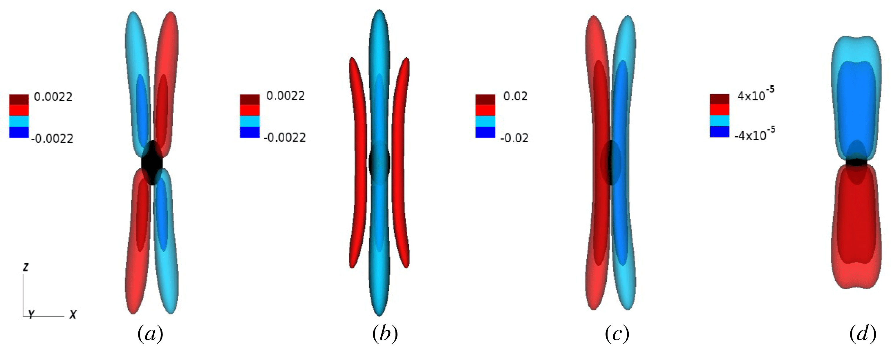
This is illustrated in figure 11 for the case of $\unicode[STIX]{x1D6FC}=2$ , taken from Davidson & Ranjan (Reference Davidson and Ranjan2018). The figure shows the results of direct numerical simulation of the full Navier–Stokes equation, including viscous forces. The buoyancy field is advected by an advection–diffusion equation, with a diffusivity $\unicode[STIX]{x1D705}$ equal to the viscosity. Figure 11 shows the results for the case of $\unicode[STIX]{x1D717}_{0}g/2\unicode[STIX]{x1D6FA}^{2}\unicode[STIX]{x1D6FF}=0.01$ , an Ekman number of $Ek=\unicode[STIX]{x1D708}/\unicode[STIX]{x1D6FA}\unicode[STIX]{x1D6FF}^{2}=0.029$ , and at time $\unicode[STIX]{x1D6FA}t=8$ . Note that the vertical jump conditions and general flow structure are as expected, with negative (positive) helicity dispersing upward (downward).

Figure 11.

The dispersion pattern from a Gaussian blob for the case of $\unicode[STIX]{x1D6FC}=2$ and $\unicode[STIX]{x1D6FA}t=8$ . Iso-surfaces of (a) $u_{z}$ , (b) $u_{y}$ , (c) $\unicode[STIX]{x1D714}_{z}$ and (d) $h$ . (From Davidson & Ranjan Reference Davidson and Ranjan2018.)

3.2 The dispersal of helicity from a buoyant layer at low $Ro$

Let us now consider a layer of buoyant blobs. Figure 12, which is taken from Davidson & Ranjan (Reference Davidson and Ranjan2015), shows the flow resulting from a random distribution of buoyant blobs concentrated in a horizontal layer and drifting slowly in the $x$ direction.

Figure 12.

Dispersion of wave energy from a layer of random buoyant blobs. The panels show iso-surfaces of $u_{z}$ (red for $u_{z}>0$ , blue for $u_{z}<0$ ) at $\unicode[STIX]{x1D6FA}t=2$ , 4, 6, 8, 10, 12. (Davidson & Ranjan Reference Davidson and Ranjan2015).

The images show the distribution of axial velocity and, as expected, we see that the inertial waves disperse in the form of axially elongated wave packets, arranged as cyclone–anticyclone pairs. It is striking that the overall flow pattern is reminiscent of that seen in the numerical dynamos (figure 1 a), and also the rotating convection study of Stellmach & Hansen (Reference Stellmach and Hansen2004). Of course, the wave packets carry negative helicity upward and positive helicity downward and Davidson & Ranjan (Reference Davidson and Ranjan2015) observe that this helicity is close to maximal, with $|h|\approx 0.85|\boldsymbol{u}||\unicode[STIX]{x1D74E}|$ . In short, we have a robust mechanism not only for the generation of helicity by buoyant blobs, but also for the spatial segregation of regions of positive and negative helicity. This provides a simple mechanism for the maintenance of a mean-field dynamo through the $\unicode[STIX]{x1D6FC}$ -effect.

That such waves are present in the numerical dynamos is clear from the study of Ranjan et al. (Reference Ranjan, Davidson, Christensen and Wicht2018). For example, figure 13 shows the $(z,t)$ space–time Fourier transform of $\unicode[STIX]{x2202}u_{z}/\unicode[STIX]{x2202}t$ at a given cylindrical radius in a reasonably supercritical numerical dynamo. (It so happens that $\unicode[STIX]{x2202}u_{z}/\unicode[STIX]{x2202}t$ is a good diagnostic for detecting wave fronts.) The horizontal axis is $\unicode[STIX]{x1D71B}/\unicode[STIX]{x1D6FA}$ and the most striking feature of this space–time transform is that the frequency is more or less restricted to the range $-2\unicode[STIX]{x1D6FA}<\unicode[STIX]{x1D71B}<2\unicode[STIX]{x1D6FA}$ , consistent with the dispersion relationship for inertial waves. Ranjan et al. (Reference Ranjan, Davidson, Christensen and Wicht2018) also show that, in the same numerical dynamo, there are more waves propagating away from the equatorial plane than towards it, consistent with the suggestion that the equatorial regions are preferentially excited by the local buoyancy flux. Moreover, there is a strong spatial correlation between the helicity and the buoyant sources of waves, as shown in Davidson & Ranjan (Reference Davidson and Ranjan2018). Interestingly, many of the columnar vortices in this numerical dynamo are internal structures, in the sense that they do not span the core, especially close to the tangent cylinder.

Figure 13.

The $(z,t)$ space–time Fourier transform of $\unicode[STIX]{x2202}u_{z}/\unicode[STIX]{x2202}t$ at a given cylindrical radius in a numerical dynamo. (From Ranjan et al. Reference Ranjan, Davidson, Christensen and Wicht2018.)

So far we have neglected the dynamical consequences of a background magnetic field. When such a field is present, a wide class of magnetic-Coriolis waves may be realised (Moffatt Reference Moffatt1978). However, these behave in much the same way as inertial waves in the sense that they are all helical, they all carry negative helicity upward and positive helicity downward and, when the local magnetic field can be treated as uniform, the radiation from a localised source is self-focussing (Bardsley & Davidson Reference Bardsley and Davidson2016). The main differences between inertial waves and magnetic-Coriolis waves is that, in the latter case, the wave packets are flattened along the line of the magnetic field (figure 14) and the group velocity is reduced. However, in a zero-order sense, this does not change the cartoon of a mean-field dynamo driven by helical waves launched in and around the equatorial plane (Bardsley & Davidson Reference Bardsley and Davidson2017).

We now discuss the mean e.m.f. and ohmic dissipation generated by these helical wave packets as they pass through an ambient magnetic field.

Figure 14.

This is the same simulation as shown in figure 12, but includes the low- $R_{m}$ Lorentz force. The magnetic field is in the $x$ direction. (From Davidson & Ranjan Reference Davidson and Ranjan2015.)

4.1 From integral kinematics to first-order smoothing

As a prelude to estimating the mean-field e.m.f. generated by helical wave packets, we wish to show that first-order smoothing is appropriate in such a calculation. To this end, we invoke an integral relationship which comes from combining (1.1) with the induction equation,

(4.1) $$\begin{eqnarray}\displaystyle & \displaystyle {\displaystyle \frac{\unicode[STIX]{x2202}\boldsymbol{B}}{\unicode[STIX]{x2202}t}}=\unicode[STIX]{x1D735}\times (\boldsymbol{u}\times \boldsymbol{B})+\unicode[STIX]{x1D706}\unicode[STIX]{x1D6FB}^{2}\boldsymbol{B}, & \displaystyle\end{eqnarray}$$

and whose derivation may be found in Davidson (Reference Davidson2013a ). It is

(4.2) $$\begin{eqnarray}\displaystyle & \displaystyle {\displaystyle \frac{\text{d}}{\text{d}t}}\int _{V_{C}}(R_{C}^{2}-\boldsymbol{x}^{2})\boldsymbol{B}\,\text{d}V=2\int _{V_{C}}\boldsymbol{x}\times (\boldsymbol{u}\times \boldsymbol{B})\,\text{d}V-6\unicode[STIX]{x1D706}\int _{V_{C}}\boldsymbol{B}\,\text{d}V. & \displaystyle\end{eqnarray}$$

This yields a sort of global evolution equation for the axial magnetic field,

(4.3) $$\begin{eqnarray}\displaystyle & \displaystyle {\displaystyle \frac{\text{d}}{\text{d}t}}\int _{V_{C}}(R_{C}^{2}-\boldsymbol{x}^{2})B_{z}\,\text{d}V=2\int _{V_{C}}r(\boldsymbol{u}\times \boldsymbol{B})_{\unicode[STIX]{x1D703}}\,\text{d}V-6\unicode[STIX]{x1D706}\int _{V_{C}}B_{z}\,\text{d}V. & \displaystyle\end{eqnarray}$$

Evidently, the mean axial field is maintained by the volume integral of $r(\boldsymbol{u}\times \boldsymbol{B})_{\unicode[STIX]{x1D703}}$ . Let us write $\boldsymbol{B}=\langle \boldsymbol{B}\rangle +\boldsymbol{b}$ and $\boldsymbol{u}=\langle \boldsymbol{u}\rangle +\boldsymbol{v}$ , where $\langle \boldsymbol{B}\rangle$ and $\langle \boldsymbol{u}\rangle$ are azimuthal averages of $\boldsymbol{B}$ and $\boldsymbol{u}$ , and $\boldsymbol{b}$ and $\boldsymbol{v}$ are the local fields associated with the columnar eddies. Then Cowling’s theorem tells us that the contributions from $\langle \boldsymbol{B}\rangle$ and $\langle \boldsymbol{u}\rangle$ to the first integral on the right of (4.3) are zero, and so,

(4.4) $$\begin{eqnarray}\displaystyle & \displaystyle {\displaystyle \frac{\text{d}}{\text{d}t}}\int _{V_{C}}(R_{C}^{2}-\boldsymbol{x}^{2})\langle B_{z}\rangle \,\text{d}V=2\int _{V_{C}}r\langle \boldsymbol{v}\times \boldsymbol{b}\rangle _{\unicode[STIX]{x1D703}}\,\text{d}V-6\unicode[STIX]{x1D706}\int _{V_{C}}\langle B_{z}\rangle \,\text{d}V. & \displaystyle\end{eqnarray}$$

Consequently, in a statistically steady dynamo, we have $R_{C}\langle \boldsymbol{v}\times \boldsymbol{b}\rangle _{\unicode[STIX]{x1D703}}\sim \unicode[STIX]{x1D706}\langle B_{z}\rangle$ , from which

(4.5) $$\begin{eqnarray}\displaystyle & \displaystyle \langle \boldsymbol{v}\times \boldsymbol{b}\rangle _{\unicode[STIX]{x1D703}}\sim {\displaystyle \frac{\unicode[STIX]{x1D706}}{|\boldsymbol{u}|R_{C}}}|\boldsymbol{u}|\langle B_{z}\rangle \ll |\boldsymbol{u}|\langle B_{z}\rangle . & \displaystyle\end{eqnarray}$$

Here $\langle \boldsymbol{v}\times \boldsymbol{b}\rangle _{\unicode[STIX]{x1D703}}$ is the mean azimuthal e.m.f. associated with the columnar eddies via the $\unicode[STIX]{x1D6FC}$ -effect. This suggests that the perturbation field $\boldsymbol{b}$ is much weaker than the mean dipole field $\langle B_{z}\rangle$ .

A similar integral relationship can be derived for the mean east–west field integrated over a hemisphere. The derivation is given in Davidson & Ranjan (Reference Davidson and Ranjan2015), who conclude that, for a quasi-steady $\unicode[STIX]{x1D6FC}^{2}$ -dynamo with negligible $\unicode[STIX]{x1D6FA}$ -effect,

(4.6) $$\begin{eqnarray}\displaystyle & \displaystyle \int _{V_{\pm }}{\displaystyle \frac{z}{r}}\langle \boldsymbol{v}\times \boldsymbol{b}\rangle _{r}\,\text{d}V\sim \unicode[STIX]{x1D706}\int _{V_{\pm }}{\displaystyle \frac{1}{r}}\langle B_{\unicode[STIX]{x1D703}}\rangle \,\text{d}V, & \displaystyle\end{eqnarray}$$

where $V_{\pm }$ may be either the northern hemisphere or the southern hemisphere. This implies that the mean azimuthal field is supported by the radial e.m.f., $\langle \boldsymbol{v}\times \boldsymbol{b}\rangle _{r}$ , as shown in figure 3. Moreover, it implies that

(4.7) $$\begin{eqnarray}\displaystyle & \displaystyle \langle \boldsymbol{v}\times \boldsymbol{b}\rangle _{r}\sim {\displaystyle \frac{\unicode[STIX]{x1D706}}{|\boldsymbol{u}|R_{C}}}|\boldsymbol{u}|\langle B_{\unicode[STIX]{x1D703}}\rangle \ll |\boldsymbol{u}|\langle B_{\unicode[STIX]{x1D703}}\rangle . & \displaystyle\end{eqnarray}$$

We conclude from (4.5) and (4.7) that $|\boldsymbol{b}|\ll |\langle \boldsymbol{B}\rangle |$ , as required for first-order smoothing in mean-field theory.

4.2 The mean-field e.m.f. induced by helical wave packets

We now estimate the e.m.f. induced by a helical wave packet passing through an ambient magnetic field. We shall assume that, as in classical mean-field theory, the transverse dimension of the columnar eddies, $\unicode[STIX]{x1D6FF}$ , is much less than $R_{C}$ , so that $\langle \boldsymbol{B}\rangle$ varies slowly on the scale of $\unicode[STIX]{x1D6FF}$ and may be treated as locally uniform. (We now use angled brackets to indicate a local spatial average.) Since the analysis is local, it is convenient to adopt Cartesian coordinates with $z$ aligned with the rotation axis. Moreover, we shall take advantage of the fact that this motion takes the form of long, thin columnar structures aligned with the $\unicode[STIX]{x1D6FA}$ . To that end, we make the following additional assumptions:

1. (i) axial gradients in $\boldsymbol{v}$ are small and so locally $\boldsymbol{v}\approx \boldsymbol{v}(x,y)$ ;

2. (ii) the fluctuations in velocity have maximal helicity, as would be the case for inertial or magnetic-Coriolis wave packets;

3. (iii) locally, the fluctuations may be treated as statistically homogeneous;

4. (iv) $|\boldsymbol{b}|\ll \langle \boldsymbol{B}\rangle$ , so that first-order smoothing may be applied.

These turn out to be reasonable approximations for a sea of inertial wave packets generated by a layer of random buoyant anomalies, as discussed in Davidson & Ranjan (Reference Davidson and Ranjan2015).

Note that assumption (ii) above gives us $\boldsymbol{c}=\boldsymbol{v}\unicode[STIX]{x1D6FF}=\unicode[STIX]{x1D74E}\unicode[STIX]{x1D6FF}^{2}$ , where $\unicode[STIX]{x1D74E}=\unicode[STIX]{x1D735}\times \boldsymbol{v}$ , $\boldsymbol{c}$ is the solenoidal vector potential for $\boldsymbol{v}$ , and we allow $\unicode[STIX]{x1D6FF}$ to be positive or negative, depending on the sign of the helicity. Note also that combining assumptions (i) and (ii) in the form $\boldsymbol{v}=\boldsymbol{v}(x,y)=\unicode[STIX]{x1D74E}\unicode[STIX]{x1D6FF}$ , and invoking statistical homogeneity, yields, after a little algebra

(4.8a,b ) $$\begin{eqnarray}\displaystyle & \displaystyle \langle \unicode[STIX]{x1D710}_{x}\unicode[STIX]{x1D710}_{z}\rangle =\langle \unicode[STIX]{x1D710}_{y}\unicode[STIX]{x1D710}_{z}\rangle =0,\quad \langle \unicode[STIX]{x1D710}_{z}^{2}\rangle =\langle \unicode[STIX]{x1D710}_{x}^{2}+\unicode[STIX]{x1D710}_{y}^{2}\rangle . & \displaystyle\end{eqnarray}$$

Turning now to the induction equation (4.1), this uncurls to give,

(4.9) $$\begin{eqnarray}\displaystyle & \displaystyle {\displaystyle \frac{\unicode[STIX]{x2202}\boldsymbol{A}}{\unicode[STIX]{x2202}t}}=\boldsymbol{u}\times \boldsymbol{B}-\unicode[STIX]{x1D735}\unicode[STIX]{x1D6F7}-\unicode[STIX]{x1D706}\unicode[STIX]{x1D735}\times \boldsymbol{B}, & \displaystyle\end{eqnarray}$$

where $\boldsymbol{A}$ is the solenoidal vector potential for $\boldsymbol{B}$ and $\unicode[STIX]{x1D6F7}$ is a scalar potential. Next we write, $\boldsymbol{u}=\langle \boldsymbol{u}\rangle +\boldsymbol{v}$ , $\boldsymbol{A}=\langle \boldsymbol{A}\rangle +\boldsymbol{a}$ and $\unicode[STIX]{x1D6F7}=\langle \unicode[STIX]{x1D6F7}\rangle +\unicode[STIX]{x1D719}$ , subtract the averaged version of (4.9) from the un-averaged version and apply first-order smoothing. This yields

(4.10) $$\begin{eqnarray}\displaystyle & \displaystyle {\displaystyle \frac{\unicode[STIX]{x2202}\boldsymbol{a}}{\unicode[STIX]{x2202}t}}=\boldsymbol{v}\times \langle \boldsymbol{B}\rangle -\unicode[STIX]{x1D735}\unicode[STIX]{x1D719}-\unicode[STIX]{x1D706}\unicode[STIX]{x1D735}\times \boldsymbol{b}, & \displaystyle\end{eqnarray}$$

where the potential $\unicode[STIX]{x1D719}$ is governed by,

(4.11) $$\begin{eqnarray}\displaystyle & \displaystyle \unicode[STIX]{x1D6FB}^{2}\unicode[STIX]{x1D719}=\langle \boldsymbol{B}\rangle \boldsymbol{\cdot }\unicode[STIX]{x1D735}\times \boldsymbol{v}=-\unicode[STIX]{x1D6FB}^{2}(\langle \boldsymbol{B}\rangle \boldsymbol{\cdot }\boldsymbol{c}), & \displaystyle\end{eqnarray}$$

or equivalently,

(4.12a,b ) $$\begin{eqnarray}\displaystyle & \displaystyle \unicode[STIX]{x1D719}=-\langle \boldsymbol{B}\rangle \boldsymbol{\cdot }\boldsymbol{c}+\hat{\unicode[STIX]{x1D719}},\quad \unicode[STIX]{x1D6FB}^{2}\hat{\unicode[STIX]{x1D719}}=0. & \displaystyle\end{eqnarray}$$

However, statistical homogeneity requires $\hat{\unicode[STIX]{x1D719}}=0$ , and so $\unicode[STIX]{x1D719}=-\langle \boldsymbol{B}\rangle \boldsymbol{\cdot }\boldsymbol{c}$ , from which,

(4.13) $$\begin{eqnarray}\displaystyle & \displaystyle \langle \unicode[STIX]{x1D719}\unicode[STIX]{x1D74E}\rangle =-\langle (\langle \boldsymbol{B}\rangle \boldsymbol{\cdot }\boldsymbol{c})\unicode[STIX]{x1D74E}\rangle =-\langle (\langle \boldsymbol{B}\rangle \boldsymbol{\cdot }\boldsymbol{v})\boldsymbol{v}\rangle . & \displaystyle\end{eqnarray}$$

Moreover, from (4.10) we have,

(4.14) $$\begin{eqnarray}\displaystyle & \displaystyle [\unicode[STIX]{x2202}/\unicode[STIX]{x2202}t-\unicode[STIX]{x1D706}\unicode[STIX]{x1D6FB}^{2}](\boldsymbol{a}-\,\boldsymbol{b}\unicode[STIX]{x1D6FF})=0, & \displaystyle\end{eqnarray}$$

and so even if b starts out as non-helical, it eventually becomes helical. We shall therefor take $\boldsymbol{a}=\boldsymbol{b}\unicode[STIX]{x1D6FF}$ , which in any case is exact for monochromatic magnetic-Coriolis waves. Equation (4.10) now becomes

(4.15) $$\begin{eqnarray}\displaystyle & \displaystyle {\displaystyle \frac{\unicode[STIX]{x2202}\boldsymbol{b}}{\unicode[STIX]{x2202}t}}+{\displaystyle \frac{\unicode[STIX]{x1D706}}{\unicode[STIX]{x1D6FF}^{2}}}\boldsymbol{b}={\displaystyle \frac{1}{\unicode[STIX]{x1D6FF}}}[\boldsymbol{v}\times \langle \boldsymbol{B}\rangle -\unicode[STIX]{x1D735}\unicode[STIX]{x1D719}], & \displaystyle\end{eqnarray}$$

which yields

(4.16) $$\begin{eqnarray}\displaystyle & \displaystyle \boldsymbol{v}\times \boldsymbol{b}+{\displaystyle \frac{\unicode[STIX]{x1D6FF}^{2}}{\unicode[STIX]{x1D706}}}\boldsymbol{v}\times \dot{\boldsymbol{b}}={\displaystyle \frac{\unicode[STIX]{x1D6FF}}{\unicode[STIX]{x1D706}}}[\boldsymbol{v}\times (\boldsymbol{v}\times \langle \boldsymbol{B}\rangle )+\unicode[STIX]{x1D735}\times (\unicode[STIX]{x1D719}\boldsymbol{v})-\unicode[STIX]{x1D719}\unicode[STIX]{x1D735}\times \boldsymbol{v}], & \displaystyle\end{eqnarray}$$

where the dot indicates a time derivative. Averaging, and eliminating $\unicode[STIX]{x1D719}\unicode[STIX]{x1D735}\times \boldsymbol{v}$ using (4.13), gives us,

(4.17) $$\begin{eqnarray}\displaystyle & \displaystyle \langle \boldsymbol{v}\times \boldsymbol{b}\rangle +{\displaystyle \frac{\unicode[STIX]{x1D6FF}^{2}}{\unicode[STIX]{x1D706}}}\langle \boldsymbol{v}\times \dot{\boldsymbol{b}}\rangle =-{\displaystyle \frac{\unicode[STIX]{x1D6FF}}{\unicode[STIX]{x1D706}}}\langle \boldsymbol{v}^{2}\langle \boldsymbol{B}\rangle -2(\boldsymbol{v}\boldsymbol{\cdot }\langle \boldsymbol{B}\rangle )\boldsymbol{v}\rangle . & \displaystyle\end{eqnarray}$$

The final step is to use (4.8) to rewrite this in the form

(4.18) $$\begin{eqnarray}\displaystyle & \displaystyle \langle \boldsymbol{v}\times \boldsymbol{b}\rangle +{\displaystyle \frac{\unicode[STIX]{x1D6FF}^{2}}{\unicode[STIX]{x1D706}}}\langle \boldsymbol{v}\times \dot{\boldsymbol{b}}\rangle =-{\displaystyle \frac{2\unicode[STIX]{x1D6FF}}{\unicode[STIX]{x1D706}}}\langle \boldsymbol{v}_{\bot }^{2}\langle \boldsymbol{B}\rangle _{\bot }-(\boldsymbol{v}_{\bot }\boldsymbol{\cdot }\langle \boldsymbol{B}\rangle _{\bot })\boldsymbol{v}_{\bot }\rangle , & \displaystyle\end{eqnarray}$$

where $\langle \boldsymbol{B}\rangle _{\bot }$ and $\boldsymbol{v}_{\bot }$ are the components of $\langle \boldsymbol{B}\rangle$ and $\boldsymbol{v}$ which are perpendicular to the rotation axis. Note that there is no source of mean e.m.f. in the direction of $\unicode[STIX]{x1D734}$ . If we additionally assume statistical symmetry about $\unicode[STIX]{x1D734}$ then $\langle \unicode[STIX]{x1D710}_{x}\unicode[STIX]{x1D710}_{y}\rangle =0$ and $\langle \unicode[STIX]{x1D710}_{x}^{2}\rangle =\langle \unicode[STIX]{x1D710}_{y}^{2}\rangle$ , which gives the simpler expression (Davidson Reference Davidson2016),

(4.19) $$\begin{eqnarray}\displaystyle & \displaystyle \langle \boldsymbol{v}\times \boldsymbol{b}\rangle +{\displaystyle \frac{\unicode[STIX]{x1D6FF}^{2}}{\unicode[STIX]{x1D706}}}\langle \boldsymbol{v}\times \dot{\boldsymbol{b}}\rangle =-{\displaystyle \frac{\unicode[STIX]{x1D6FF}}{2\unicode[STIX]{x1D706}}}\langle \boldsymbol{v}^{2}\rangle \langle \boldsymbol{B}\rangle _{\bot }=-{\displaystyle \frac{\unicode[STIX]{x1D6FF}^{2}}{2\unicode[STIX]{x1D706}}}\langle h\rangle \langle \boldsymbol{B}\rangle _{\bot }. & \displaystyle\end{eqnarray}$$

The low- $R_{m}$ version of this, $\langle \boldsymbol{v}\times \boldsymbol{b}\rangle =-(\unicode[STIX]{x1D6FF}^{2}/2\unicode[STIX]{x1D706})\langle h\rangle \langle \boldsymbol{B}\rangle _{\bot }$ , has been tested against the numerical simulation shown in figure 12 and found to be reasonably accurate (Davidson & Ranjan Reference Davidson and Ranjan2015).

4.3 A mean-field estimate of the ohmic dissipation induced by helical wave packets

For our scaling analysis in § 5, we will need an estimate of the ohmic dissipation, so let us now calculate the dissipation caused by the passage of columnar wave packets through a mean magnetic field. We start by rewriting (4.15) in the form

(4.20) $$\begin{eqnarray}\displaystyle & \displaystyle \boldsymbol{j}+{\displaystyle \frac{\unicode[STIX]{x1D6FF}^{2}}{\unicode[STIX]{x1D706}}}{\displaystyle \frac{\unicode[STIX]{x2202}\boldsymbol{j}}{\unicode[STIX]{x2202}t}}=\unicode[STIX]{x1D70E}[\boldsymbol{v}\times \langle \boldsymbol{B}\rangle -\unicode[STIX]{x1D735}\unicode[STIX]{x1D719}], & \displaystyle\end{eqnarray}$$

where $\unicode[STIX]{x1D707}\boldsymbol{j}=\unicode[STIX]{x1D735}\times \boldsymbol{b}$ , from which we find,

(4.21) $$\begin{eqnarray}\displaystyle & \displaystyle \boldsymbol{j}^{2}+{\displaystyle \frac{\unicode[STIX]{x1D6FF}^{2}}{\unicode[STIX]{x1D706}}}{\displaystyle \frac{\unicode[STIX]{x2202}}{\unicode[STIX]{x2202}t}}(\,\boldsymbol{j}^{2}/2)={\displaystyle \frac{\unicode[STIX]{x1D70E}}{\unicode[STIX]{x1D6FF}\unicode[STIX]{x1D707}}}[\boldsymbol{b}\boldsymbol{\cdot }(\boldsymbol{v}\times \langle \boldsymbol{B}\rangle )-\unicode[STIX]{x1D735}\boldsymbol{\cdot }(\unicode[STIX]{x1D719}\boldsymbol{b})], & \displaystyle\end{eqnarray}$$

and

(4.22) $$\begin{eqnarray}\displaystyle & \displaystyle \left({\displaystyle \frac{\unicode[STIX]{x1D6FF}^{2}}{\unicode[STIX]{x1D706}}}{\displaystyle \frac{\unicode[STIX]{x2202}\boldsymbol{j}}{\unicode[STIX]{x2202}t}}\right)^{2}+{\displaystyle \frac{\unicode[STIX]{x1D6FF}^{2}}{\unicode[STIX]{x1D706}}}{\displaystyle \frac{\unicode[STIX]{x2202}}{\unicode[STIX]{x2202}t}}(\,\boldsymbol{j}^{2}/2)={\displaystyle \frac{\unicode[STIX]{x1D70E}}{\unicode[STIX]{x1D6FF}\unicode[STIX]{x1D707}}}{\displaystyle \frac{\unicode[STIX]{x1D6FF}^{2}}{\unicode[STIX]{x1D706}}}\left[{\displaystyle \frac{\unicode[STIX]{x2202}\boldsymbol{b}}{\unicode[STIX]{x2202}t}}\boldsymbol{\cdot }(\boldsymbol{v}\times \langle \boldsymbol{B}\rangle )-\unicode[STIX]{x1D735}\boldsymbol{\cdot }\left(\unicode[STIX]{x1D719}{\displaystyle \frac{\unicode[STIX]{x2202}\boldsymbol{b}}{\unicode[STIX]{x2202}t}}\right)\right]. & \displaystyle\end{eqnarray}$$

Adding and averaging these yields

(4.23) $$\begin{eqnarray}\displaystyle & \displaystyle {\displaystyle \frac{\unicode[STIX]{x1D6FF}\unicode[STIX]{x1D707}}{\unicode[STIX]{x1D70E}}}\left\langle \left(\boldsymbol{j}+{\displaystyle \frac{\unicode[STIX]{x1D6FF}^{2}}{\unicode[STIX]{x1D706}}}{\displaystyle \frac{\unicode[STIX]{x2202}\boldsymbol{j}}{\unicode[STIX]{x2202}t}}\right)^{2}\right\rangle ={\displaystyle \frac{\unicode[STIX]{x1D6FF}^{2}}{\unicode[STIX]{x1D706}}}\left\langle {\displaystyle \frac{\unicode[STIX]{x2202}\boldsymbol{b}}{\unicode[STIX]{x2202}t}}\boldsymbol{\cdot }(\boldsymbol{v}\times \langle \boldsymbol{B}\rangle )\right\rangle +\langle \boldsymbol{b}\boldsymbol{\cdot }(\boldsymbol{v}\times \langle \boldsymbol{B}\rangle )\rangle , & \displaystyle\end{eqnarray}$$

or equivalently,

(4.24) $$\begin{eqnarray}\displaystyle & \displaystyle {\displaystyle \frac{\unicode[STIX]{x1D6FF}\unicode[STIX]{x1D707}}{\unicode[STIX]{x1D70E}}}\left\langle \left(\boldsymbol{j}+{\displaystyle \frac{\unicode[STIX]{x1D6FF}^{2}}{\unicode[STIX]{x1D706}}}{\displaystyle \frac{\unicode[STIX]{x2202}\boldsymbol{j}}{\unicode[STIX]{x2202}t}}\right)^{2}\right\rangle =-\!\left[\langle \boldsymbol{v}\times \boldsymbol{b}\rangle +{\displaystyle \frac{\unicode[STIX]{x1D6FF}^{2}}{\unicode[STIX]{x1D706}}}\left\langle \boldsymbol{v}\times {\displaystyle \frac{\unicode[STIX]{x2202}\boldsymbol{b}}{\unicode[STIX]{x2202}t}}\right\rangle \right]\boldsymbol{\cdot }\langle \boldsymbol{B}\rangle . & \displaystyle\end{eqnarray}$$

Comparing (4.19) with (4.24) now gives us

(4.25) $$\begin{eqnarray}\displaystyle & \displaystyle {\displaystyle \frac{\unicode[STIX]{x1D707}}{\unicode[STIX]{x1D70E}}}\left\langle \left(\boldsymbol{j}+{\displaystyle \frac{\unicode[STIX]{x1D6FF}^{2}}{\unicode[STIX]{x1D706}}}{\displaystyle \frac{\unicode[STIX]{x2202}\boldsymbol{j}}{\unicode[STIX]{x2202}t}}\right)^{2}\right\rangle ={\displaystyle \frac{1}{2\unicode[STIX]{x1D706}}}\langle \boldsymbol{v}^{2}\rangle \langle \boldsymbol{B}_{\bot }^{2}\rangle , & \displaystyle\end{eqnarray}$$

while Davidson (Reference Davidson2016) shows that, for monochromatic waves, equation (4.24) simplifies to the remarkably simple result

(4.26) $$\begin{eqnarray}\displaystyle & \displaystyle {\displaystyle \frac{\unicode[STIX]{x1D707}\unicode[STIX]{x1D6FF}}{\unicode[STIX]{x1D70E}}}\langle \,\boldsymbol{j}^{2}\rangle =-\langle \boldsymbol{v}\times \boldsymbol{b}\rangle \boldsymbol{\cdot }\langle \boldsymbol{B}_{\bot }\rangle . & \displaystyle\end{eqnarray}$$

This is the key result of § 4. Note that $\unicode[STIX]{x1D6FF}>0$ (positive helicity) implies $\langle \boldsymbol{v}\times \boldsymbol{b}\rangle \boldsymbol{\cdot }\langle \boldsymbol{B}_{\bot }\rangle <0$ , while $\unicode[STIX]{x1D6FF}<0$ (negative helicity) gives $\langle \boldsymbol{v}\times \boldsymbol{b}\rangle \boldsymbol{\cdot }\langle \boldsymbol{B}_{\bot }\rangle >0$ , in line with the usual interpretation of the $\unicode[STIX]{x1D6FC}$ -effect.

5.1 Scaling laws for helical-wave dynamos

Equation (4.26) forms the basis of the dynamo scaling laws given in Davidson (Reference Davidson2016). When combined with the estimates of § 4, $R_{C}\langle \boldsymbol{v}\times \boldsymbol{b}\rangle \sim \unicode[STIX]{x1D706}\langle \boldsymbol{B}\rangle$ , we have

(5.1) $$\begin{eqnarray}\displaystyle & \displaystyle {\displaystyle \frac{1}{\unicode[STIX]{x1D70E}\unicode[STIX]{x1D70C}}}\langle \,\boldsymbol{j}^{2}\rangle \sim {\displaystyle \frac{\unicode[STIX]{x1D706}}{R_{C}\unicode[STIX]{x1D6FF}}}{\displaystyle \frac{1}{\unicode[STIX]{x1D70C}\unicode[STIX]{x1D707}}}\langle \boldsymbol{B}^{2}\rangle , & \displaystyle\end{eqnarray}$$

where we now take $\unicode[STIX]{x1D6FF}$ to be a strictly positive quantity and the left-hand side of (5.1) is the Joule dissipation per unit mass. In a statistically steady dynamo the integral of this dissipation must equal the integral of the rate of working of the buoyancy force per unit mass, $P=\langle \unicode[STIX]{x1D717}\boldsymbol{g}\boldsymbol{\cdot }\boldsymbol{u}\rangle$ , the viscous dissipation being negligible in a planetary core and relatively modest in the more recent numerical dynamos. Introducing the two velocity scales $\unicode[STIX]{x1D710}_{A}=\langle \boldsymbol{B}^{2}\rangle ^{1/2}/\sqrt{\unicode[STIX]{x1D70C}\unicode[STIX]{x1D707}}$ and $\unicode[STIX]{x1D710}_{P}=(PR_{C})^{1/3}$ , equation (5.1) becomes

(5.2) $$\begin{eqnarray}\displaystyle & \displaystyle \unicode[STIX]{x1D710}_{p}^{3}\sim {\displaystyle \frac{\unicode[STIX]{x1D706}}{\unicode[STIX]{x1D6FF}}}\unicode[STIX]{x1D710}_{A}^{2}. & \displaystyle\end{eqnarray}$$

In addition, we shall demand that the curl of the Coriolis force, which shapes the flow, is of the order of the curl of the buoyancy force, which drives the motion. So (3.4) yields

(5.3) $$\begin{eqnarray}\displaystyle & \displaystyle \unicode[STIX]{x1D734}\boldsymbol{\cdot }\unicode[STIX]{x1D735}\boldsymbol{u}\sim \unicode[STIX]{x1D735}\unicode[STIX]{x1D717}\times \boldsymbol{g}\sim \unicode[STIX]{x1D717}g/\unicode[STIX]{x1D6FF}\sim P/u\unicode[STIX]{x1D6FF}. & \displaystyle\end{eqnarray}$$

Assuming that axial gradients scale on the core radius, this yields the estimate $\unicode[STIX]{x1D710}_{p}^{3}\sim \unicode[STIX]{x1D6FA}\unicode[STIX]{x1D6FF}u^{2}$ , which combines with (5.2) to give (Davidson Reference Davidson2016)

(5.4) $$\begin{eqnarray}\displaystyle & \displaystyle \unicode[STIX]{x1D710}_{p}^{3}\sim {\displaystyle \frac{\unicode[STIX]{x1D706}}{\unicode[STIX]{x1D6FF}}}\unicode[STIX]{x1D710}_{A}^{2}\sim \unicode[STIX]{x1D6FA}\unicode[STIX]{x1D6FF}u^{2}. & \displaystyle\end{eqnarray}$$

This is our key scaling relationship. Note that it is not limited to low- $R_{m}$ and it predicts that the total energy density (magnetic plus kinetic) is of the order of

(5.5) $$\begin{eqnarray}\displaystyle & \displaystyle e\sim \unicode[STIX]{x1D710}_{A}^{2}+u^{2}\sim \unicode[STIX]{x1D710}_{P}^{3}\left[{\displaystyle \frac{\unicode[STIX]{x1D6FF}}{\unicode[STIX]{x1D706}}}+{\displaystyle \frac{1}{\unicode[STIX]{x1D6FA}\unicode[STIX]{x1D6FF}}}\right]. & \displaystyle\end{eqnarray}$$

Thus the ratio of magnetic to kinetic energy is $\unicode[STIX]{x1D6FA}\unicode[STIX]{x1D6FF}^{2}/\unicode[STIX]{x1D706}$ . Note also that we can rewrite (5.4) in terms of the small-scale Rossby number, $Ro_{\unicode[STIX]{x1D6FF}}=u/\unicode[STIX]{x1D6FA}\unicode[STIX]{x1D6FF}$ , as,

(5.6a,b ) $$\begin{eqnarray}\displaystyle & \displaystyle {\displaystyle \frac{u}{\unicode[STIX]{x1D710}_{P}}}\sim (Ro_{\unicode[STIX]{x1D6FF}})^{1/3},\quad {\displaystyle \frac{\unicode[STIX]{x1D710}_{A}}{\unicode[STIX]{x1D710}_{P}}}\sim {\displaystyle \frac{\unicode[STIX]{x1D710}_{P}}{\sqrt{\unicode[STIX]{x1D706}\unicode[STIX]{x1D6FA}}}}(Ro_{\unicode[STIX]{x1D6FF}})^{-1/3}. & \displaystyle\end{eqnarray}$$

Since inertial waves cannot propagate when $Ro_{\unicode[STIX]{x1D6FF}}$ is greater than $Ro_{\unicode[STIX]{x1D6FF}}\approx 0.4$ (see § 2.1), this places an upper bound of ${\sim}\unicode[STIX]{x1D710}_{P}$ on $u$ and a lower bound of ${\sim}\unicode[STIX]{x1D710}_{P}^{2}/\sqrt{\unicode[STIX]{x1D706}\unicode[STIX]{x1D6FA}}$ on $\unicode[STIX]{x1D710}_{A}$ for a helical-wave dynamo.

Now it is easy to show that $P$ is uniquely determined by the convective heat flux though the core of a planet. In the case of the terrestrial planets virtually all of the thermal resistance lies in the mantle, and so we may think of $P$ as prescribed and independent of the motion in the core. In the gas giants, on the other hand, $P$ may be estimated directly from their luminosity. Either way, estimates of $P$ are available for Jupiter and Saturn ( $P\approx 1.2\times 10^{-10}~\text{m}^{2}~\text{s}^{-3}$ and $P\approx 0.43\times 10^{-10}~\text{m}^{2}~\text{s}^{-3}$ , respectively, Read et al. Reference Read2015), and plausible guesses for the Earth ( $P\approx 5.1\times 10^{-13}~\text{m}^{2}~\text{s}^{-3}$ , Christensen Reference Christensen2010). So, provided $\unicode[STIX]{x1D6FF}$ is known, equation (5.4) can be used to estimate $\unicode[STIX]{x1D710}_{A}$ and $u$ , and hence the r.m.s. magnetic field and the global Rossby number. Unfortunately, we do not know what determines $\unicode[STIX]{x1D6FF}$ in the core of the planets, although we do know how $\unicode[STIX]{x1D6FF}$ scales in the numerical dynamos. So we shall first test (5.4) against the numerical dynamos and then ask what it tells us about the planets.

5.2 Testing the scaling law (5.4) against the numerical dynamos

In most of the numerical dynamos the transverse scale of the columnar eddies is set by a viscous balance, which yields $\unicode[STIX]{x1D6FF}\sim (Ek)^{1/3}R_{C}$ , (King & Buffett Reference King and Buffett2013). Our scaling laws then become

(5.7a,b ) $$\begin{eqnarray}\displaystyle & \displaystyle \unicode[STIX]{x1D6F1}_{B}\sim \unicode[STIX]{x1D6F1}_{P}^{1/2}\,\mathit{Pr}_{m}^{1/2}\,\,Ek^{-1/3},\quad Ro\sim \unicode[STIX]{x1D6F1}_{P}^{1/2}Ek^{-1/6}, & \displaystyle\end{eqnarray}$$

where

(5.8a-d ) $$\begin{eqnarray}\displaystyle & \displaystyle \unicode[STIX]{x1D6F1}_{B}={\displaystyle \frac{B_{\text{rms}}/\sqrt{\unicode[STIX]{x1D70C}\unicode[STIX]{x1D707}}}{\unicode[STIX]{x1D6FA}R_{C}}},\quad \unicode[STIX]{x1D6F1}_{p}={\displaystyle \frac{P}{\unicode[STIX]{x1D6FA}^{3}R_{C}^{2}}},\quad Ro={\displaystyle \frac{u}{\unicode[STIX]{x1D6FA}R_{C}}},\quad \mathit{Pr}_{m}={\displaystyle \frac{\unicode[STIX]{x1D708}}{\unicode[STIX]{x1D706}}}. & \displaystyle\end{eqnarray}$$

Scaling (5.7) for the global Rossby number, $Ro$ , has been proposed by several authors (e.g. King & Buffett Reference King and Buffett2013, Davidson Reference Davidson2014) and found to be a good match to numerical dynamo data sets. On the other hand, scaling (5.7) for $\unicode[STIX]{x1D6F1}_{B}$ was first proposed in Davidson (Reference Davidson2014), although in that particular paper the derivation was limited to a low magnetic Reynolds number on the scale of $\unicode[STIX]{x1D6FF}$ .

Figure 15, which is taken from Davidson (Reference Davidson2016), compares scaling laws (5.7) with a suite of numerical dynamos tabulated in Christensen & Aubert (Reference Christensen and Aubert2006). When discussing the simulations it is usual to replace $\unicode[STIX]{x1D6F1}_{P}$ and $Ek$ by the related parameters $Ra_{Q}=\unicode[STIX]{x1D6F1}_{P}/r(1-r)^{2}$ and $E=Ek/(1-r)^{2}$ , where $r$ is the ratio of the inner and outer core radii. We follow that convention in figure 15. Also, in order to allow for the viscous dissipation in the numerical dynamos, which has been ignored in the scaling analysis, $\unicode[STIX]{x1D6F1}_{B}$ has been replaced by $\unicode[STIX]{x1D6F1}_{B}/\sqrt{f_{\text{ohm}}}$ , where $f_{\text{ohm}}$ is the ratio of the Joule dissipation to the total dissipation. (This correction was introduced by Christensen & Aubert (Reference Christensen and Aubert2006), on the grounds that the scaling for $\unicode[STIX]{x1D6F1}_{B}$ is based on an energy balance, and this ignores the unphysical viscous dissipation present in the numerical dynamos.) The comparison in figure 15 is evidently favourable and offers support for the scaling laws (5.7), and by implication, support for the more general scaling (5.4).

Figure 15.

A comparison of scaling laws (5.7) with the numerical data set of Christensen & Aubert (Reference Christensen and Aubert2006). Scalings: (a) $Ro\sim \unicode[STIX]{x1D6F1}_{P}^{1/2}Ek^{-1/6}$ , (b) $\unicode[STIX]{x1D6F1}_{B}\sim \unicode[STIX]{x1D6F1}_{P}^{1/2}\,\mathit{Pr}_{m}^{1/2}\,\,Ek^{-1/3}$ . From Davidson (Reference Davidson2016).

Let us now turn to the observation that inertial waves cannot propagate when $Ro_{\unicode[STIX]{x1D6FF}}=u/\unicode[STIX]{x1D6FA}\unicode[STIX]{x1D6FF}$ is greater than ${\sim}0.4$ . If inertial waves are indeed central to maintaining a dipolar dynamo, then $Ro_{\unicode[STIX]{x1D6FF}}\approx 0.4$ should represent a transition from dipolar to multipolar dynamos. Combining $Ro\sim \unicode[STIX]{x1D6F1}_{P}^{1/2}Ek^{-1/6}$ with the viscous scaling $\unicode[STIX]{x1D6FF}/R_{C}\sim Ek^{1/3}$ , our scaling analysis predicts that $Ro_{\unicode[STIX]{x1D6FF}}\sim \unicode[STIX]{x1D6F1}_{P}^{1/2}Ek^{-1/2}$ , and in what follows we shall take the pre-factor in this estimate to be equal to unity. Combining this with the transition criterion $Ro_{\unicode[STIX]{x1D6FF}}\approx 0.4$ , and replacing $\unicode[STIX]{x1D6F1}_{P}$ and Ek by $Ra_{Q}$ and $E$ , we conclude that the transition from dipolar to multipolar dynamos in an Earth-like numerical simulation should occur at $2Ra_{Q}/E\approx 1$ . Figure 16, again taken from Davidson (Reference Davidson2016), shows $f_{\text{dip}}$ plotted as a function of $2Ra_{Q}/E$ , where $f_{\text{dip}}$ is the field strength of the dipole at the outer boundary of the simulation, divided by the field contained in the harmonics of degree 1 to 12. It is conventional to regard dipolar cases as corresponding to $f_{\text{dip}}>0.5$ , and multipolar dynamos as characterised by $f_{\text{dip}}<0.35$ . Evidently, the transition criterion $2Ra_{Q}/E\approx 1$ does a reasonable job of distinguishing between dipolar and non-dipolar dynamos, thus lending support to the hypothesis that inertial waves are crucial to maintaining a dipolar dynamo. We note in passing that the Earth lies in the wrong quadrant in figure 16, which reminds us that the scaling $\unicode[STIX]{x1D6FF}/R_{C}\sim Ek^{1/3}$ is purely an artefact of the excessive viscosity in the numerical dynamos, and does not apply to the planets.

Figure 16.

$f_{\text{dip}}$ as a function of $2Ra_{Q}/E$ for the same data set as figure 15. From Davidson (Reference Davidson2016).

5.3 Applying the scaling laws to the planets

The evidence of § 5.2 lends support for the scaling (5.4), so let us now apply it to the planets. We shall focus on the Earth and the gas giants, as their magnetic fields look somewhat similar and so it seems plausible that their dynamos operate in roughly the same manner. The ice giants, by way of contrast, have multipolar magnetic fields, while the data for Mercury are less certain.

As already noted, we do not know what sets the scale $\unicode[STIX]{x1D6FF}$ in the core of the planets, but this does not prevent us from considering different possibilities and then comparing the resulting predictions with the observational evidence. Note that it is entirely possible that the way in which $\unicode[STIX]{x1D6FF}$ is set in the gas giants is different to that in the core of the Earth, and if this is true, we have no right to expect that the same scaling laws apply to both. Still, several authors have looked for evidence of a universal scaling (e.g. Christensen, Holzwarth & Reiners Reference Christensen, Holzwarth and Reiners2009, and Davidson Reference Davidson2016), and so we shall pursue this theme.

Table 2.

A comparison of observed and predicted values of $\unicode[STIX]{x1D6F1}_{B}$ , $u$ and $\unicode[STIX]{x1D6FF}$ . We use $\unicode[STIX]{x1D706}\sim 0.7~\text{m}^{2}~\text{s}^{-1}$ , $\unicode[STIX]{x1D70C}\sim 10^{4}~\text{kg}~\text{m}^{-3}$ for the Earth, and $\unicode[STIX]{x1D706}\sim 3~\text{m}^{2}~\text{s}^{-1}$ , $\unicode[STIX]{x1D70C}\sim 10^{3}~\text{kg}~\text{m}^{-3}$ for the gas giants.

One common proposal is that $\unicode[STIX]{x1D6FF}$ is set by the criterion $u\unicode[STIX]{x1D6FF}/\unicode[STIX]{x1D706}\sim 1$ . Rather surprisingly, when combined with (5.4), this returns us to the traditional assumption, $\unicode[STIX]{x1D70E}B_{\text{rms}}^{2}/\unicode[STIX]{x1D70C}\unicode[STIX]{x1D6FA}\sim 1$ . However, it turns out that this would have the gas giants operating in a strongly multipolar regime (Davidson Reference Davidson2016). Perhaps a more attractive option is to assert that $\unicode[STIX]{x1D6FF}$ marks the transition from high- $R_{m}$ dynamics to strongly damped, low- $R_{m}$ behaviour, which occurs at a Lundquist number of $\unicode[STIX]{x1D710}_{A}\unicode[STIX]{x1D6FF}/\unicode[STIX]{x1D706}\sim 1$ . When combined with (5.4), this leads to the remarkably simple result $\unicode[STIX]{x1D710}_{A}\sim \unicode[STIX]{x1D710}_{P}$ , which has $B$ independent of $\unicode[STIX]{x1D6FA}$ . Exactly this scaling has been proposed as a universal scaling law in Christensen et al. (Reference Christensen, Holzwarth and Reiners2009), although based on a different line of reasoning. When $u$ and $\unicode[STIX]{x1D6FF}$ are also estimated from (5.4), we find

(5.9a-c ) $$\begin{eqnarray}\displaystyle \unicode[STIX]{x1D710}_{A}\sim \unicode[STIX]{x1D710}_{P},\quad u\sim \unicode[STIX]{x1D710}_{P}^{2}/\sqrt{\unicode[STIX]{x1D6FA}\unicode[STIX]{x1D706}},\quad \unicode[STIX]{x1D6FF}\sim \unicode[STIX]{x1D706}/\unicode[STIX]{x1D710}_{p},\quad \text{(scaling laws I)}. & & \displaystyle\end{eqnarray}$$

However, for the Earth these scaling laws make $\unicode[STIX]{x1D6FF}$ uncomfortably small (see table 2), and (5.9) probably places the gas giants in the multipolar regime (again, see Davidson Reference Davidson2016).

A third hypothesis is that, for a given buoyancy flux, the dynamo operates so as to minimise its magnetic energy while remaining in the dipolar regime. From (5.5) we see that this requires that we minimise $\unicode[STIX]{x1D6FF}$ subject to the constraint that $Ro_{\unicode[STIX]{x1D6FF}}\leqslant O(1)$ , i.e. the criterion is $u/\unicode[STIX]{x1D6FA}\unicode[STIX]{x1D6FF}\sim 1$ . As with (5.9), this makes $\unicode[STIX]{x1D6FF}$ rather small for the Earth (less than a kilometre), but it does have the virtue of keeping the gas giants in the dipolar regime. Combining $u/\unicode[STIX]{x1D6FA}\unicode[STIX]{x1D6FF}\sim 1$ with (5.6) yields the estimates

(5.10a-c ) $$\begin{eqnarray}\displaystyle & \displaystyle u\sim \unicode[STIX]{x1D710}_{P},\quad \unicode[STIX]{x1D710}_{A}\sim \unicode[STIX]{x1D710}_{P}^{2}/\sqrt{\unicode[STIX]{x1D6FA}\unicode[STIX]{x1D706}},\quad \unicode[STIX]{x1D6FF}\sim \unicode[STIX]{x1D710}_{p}/\unicode[STIX]{x1D6FA},\quad \text{(scaling laws II)}, & \displaystyle\end{eqnarray}$$

which have the roles of $u$ and $\unicode[STIX]{x1D710}_{A}$ reversed relative to (5.9). In terms of $\unicode[STIX]{x1D6F1}_{B}$ , equation (5.10) predicts

(5.11) $$\begin{eqnarray}\displaystyle & \displaystyle \unicode[STIX]{x1D6F1}_{B}={\displaystyle \frac{B_{\text{rms}}/\sqrt{\unicode[STIX]{x1D70C}\unicode[STIX]{x1D707}}}{\unicode[STIX]{x1D6FA}R_{C}}}\sim {\displaystyle \frac{\unicode[STIX]{x1D710}_{P}}{\unicode[STIX]{x1D6FA}R_{C}}}{\displaystyle \frac{\unicode[STIX]{x1D710}_{P}}{\sqrt{\unicode[STIX]{x1D6FA}\unicode[STIX]{x1D706}}}}. & \displaystyle\end{eqnarray}$$

In table 2 we compare these two sets of scaling laws with the observational data for the Earth, Jupiter and Saturn, taking the pre-factor in all of these relationships to be equal to unity. In doing so we make the crude estimate $B_{\text{rms}}=10\bar{B}_{z}$ , which is 37 Gauss for the case of the Earth. (Thirty-seven Gauss is consistent with estimates based on the observed frequency of torsional oscillations in the core.) Given the uncertainties in the values of the magnetic diffusivities, especially for the gas giants, and in the estimates of the various convective heat fluxes, the scaling laws in (5.10) compare favourably with the observations. By comparison, the scalings in (5.9) are less attractive, partly because of the implausibly small values for $\unicode[STIX]{x1D6FF}$ that result, and partly because $u/\unicode[STIX]{x1D6FA}\unicode[STIX]{x1D6FF}$ is predicted to be larger than unity, which is inconsistent with a dipolar field. It should be emphasised, however, that the entire issue of the existence of universal scaling laws for the planets remains an open question.