I. INTRODUCTION
Woven fabric composites are widely used as structural components in aerospace, automobile, and boat industries due to their high specific stiffness and high specific strength as well as their improved resistance to impact. When these composites are used in main parts of structures, they are expected to experience a range of mechanical, thermal, and chemical environment during their service life. Since woven fabric composites have been used in primary structural applications, an accurate evaluation of their mechanical and thermal properties becomes important. Woven fabrics in a woven fabric composite are usually made of interlaced yarns and the distribution of fibers in the yarns. The properties of woven fabric composites depend on (i) constituent volume fraction, (ii) yarn undulation, (iii) the shape of yarn cross-section, (iv) yarn spacing, (v) weave style, and (vi) properties of the constituent materials. The weave styles are diverse such as biaxial weave or triaxial weave. For orthogonally biaxial weave, the change of the weaving of warp and weft yarns leads to different woven patterns, such as plain weave, twill weave, or various harness satin weaves.Reference Tang, Whitcomb, Li and Sue1 The packing of the fibers in the yarns is random. Because of their complicated architecture and anisotropic nature, it is difficult to fully predict the mechanical and thermal characteristics of these materials from the results of mechanical and thermal tests. Therefore, it is necessary to conduct reliable numerical simulations to evaluate their mechanical and thermal behavior.
The numerical simulations are usually carried out via the use of the finite element method. The analytical models used to represent these composites are either homogenous, or heterogeneous in nature. The use of homogenous models is limited to the macroscopic evaluation of the properties of composites. Heterogeneous models, which include two-dimensional (2D)Reference Li2 and three-dimensional (3D) models,Reference Li and Wongsto3 are dedicated to the microscopic evaluation of their properties. A 2D model with generalized plane strain condition is acceptable when a composite is a unidirectional (UD) fiber reinforced composite. However, these simplified conditions are not correct when we deal with structures such as woven fabric composites. For such structures, a 3D modeling becomes necessary. The 3D micromechanical finite element analyses or heat transfer analyses of woven fabric composites are generally used to obtain the effective engineering properties such as effective moduli, Poisson’s ratios, thermal expansion coefficients,Reference Li, Li, Wang, Kandare, Kandola, Myler and Horrocks4 or thermal conductivities, which are needed for macrolevel analyses of composite structures.
Prediction of composite effective properties based on the constituent material properties and microarchitecture of the reinforcement has been of interest for many years. Unidirectional and particulate composites have been extensively studied in the past. However, few numerical studies are available for effective thermal properties of woven fabric composites.Reference Dasgupta, Agarwal and Bhandarkar5 Dasgupta et al.Reference Dasgupta, Agarwal and Bhandarkar5, Reference Dasgupta and Agarwal6 first predicted the orthotropic thermal conductivity of plain weave fabric composites using a homogenization technique. Temperature boundary conditions are used to obtain an upper bound estimate of the thermal conductivity and flux boundary conditions are used for the lower bound for 3D finite element analyses. Bigaud et al.Reference Bigaud, Goyheneche and Hamelin7 have provided a way to calculate the effective thermal conductivity tensor of textile-reinforced composites. Woo and GooReference Woo and Goo8 have performed experiments and analyses to obtain the thermal conductivity of carbon-phenolic 8-harness satin weave composites. Periodicity vectors for the boundary conditions of representative volume element were applied to finite element analyses. Farooqi and SheikhReference Farooqi and Sheikh9 have calculated the effective thermal conductivity of ceramic-matrix composites. The boundary conditions for their models were one-dimensional heat flow in steady-state and transient cases. Schuster et al.Reference Schuster, Heider, Sharp and Glowania10 have investigated finite element analyses to calculate the out-of-plane thermal conductivity of woven fabric composites.
This work focuses on systematically calculating the effective thermal conductivities of woven fabric composites using two unit cells with periodic boundary conditions. The distribution of the fibers in the yarns and of the yarns in a woven fabric composite has a regular feature; the composite material is then idealized as a patterned array of identical cells, often referred to as unit cells at a meso-microsopic or macro-mesoscopic scale. This allows us to apply periodic boundary conditions to the unit cells. Two different unit cells derived from inherently periodic geometries of woven fabric composites are used. One unit cell with periodic boundary conditions is first applied to investigate the meso-microsopic material behavior of a single yarn based on the properties of the constituent phases. Another unit cell is then built to enclose the characteristic periodic pattern in the woven fabric composites to investigate their macro-mesoscopic material behavior. The two unit cells are referred to as Unit Cell 1 (meso-microsopic scale) and Unit Cell 2 (macro-mesoscopic scale); both based on the use of translational symmetry transformations only. Periodic boundary conditions for the two unit cells are derived from appropriate considerations of the temperature relations resulting from translational symmetry transformations before carrying out finite element analyses. After heat transfer analyses of the Unit Cell 2, the effective thermal conductivities of woven fabric composites have been evaluated.
II. METHODOLOGY
In this work, the heat transfer analyses of woven fabric composites will be carried out to obtain the effective thermal conductivities of the composites using two unit cells established at different length scales. The following two hypotheses are assumed before the heat transfer analyses: (i) periodic distribution of the fibers in the yarns, (ii) periodic arrangement of the reinforcing yarns in the woven fabric composites. The first hypothesis concerns a representative volume of an UD yarn. Untwisted UD fibers bonded by resin form the yarn. The effective properties of such yarn are the objective of Unit Cell 1 and will be passed into Unit Cell 2 as input data. The second hypothesis deals with a representative volume of a layer in a woven fabric composite. The interwoven yarns, once assembled according to designated patterns and bonded together by resin, form a layer in a laminated composite. Unit Cell 2 is introduced to evaluate the effective properties of such a layer. Considering the layer represented by Unit Cell 2 as a lamina in a laminated composite, the overall behavior of the composite can be described using an appropriate laminate theory to predict the performances of structures made of such composite.
A. Unit Cell 1—A hexagon
Yarns with fibers bonded by resin form an UD composite. However, the interwoven pattern in a woven fabric composite introduces various degrees of waviness. The scale of undulations of yarns is usually much greater than that of fiber diameters and therefore yarns in a woven composite can be reasonably idealized as an UD fiber-reinforced composite. The effects of waviness will be taken into account in Unit Cell 2, and will be introduced in Sec. III. B, which shares the same length scale of the undulations of yarns. A single yarn is made of thousands of fibers. If a cross section of a yarn is examined, the fibers show a reasonably circular shape with a fairly uniform diameter. The shape of the yarn cross-sections is mainly influenced by the laying out of the fibers. The distribution of fibers in the plane of the cross section is usually completely at random. As an idealization, a regular arrangement can be introduced. For regular array of uniform fibers at the cross section of a yarn, square and hexagonal cells obtained via Voronoi tessellations are normally taken as unit cells.Reference Ahuja and Schachter11 The cells obtained from Voronoi tessellations can be described as domains enclosed by bisecting sides of the segment connecting the center of the cell and those of the neighboring cells. All Voronoi cells are identical throughout the plane and any one cell can be reproduced by another through a certain translational symmetry transformation. Under translational symmetry transformations alone, relative temperatures, temperature gradients, and heat fluxes are transformed identically from the unit cell to any other cell as the images of those in the unit cell. Therefore, temperature fields and heat flux fields are distributed identically in a unit cell and any other unit cell. As a result, any Voronoi cell can be chosen as the unit cell. The superiority of the hexagonal packing to the square packing is that it preserves transverse isotropy, which a real composite possesses in a statistical sense due to the random distribution of fibers in the matrix over the cross section of a yarn, whereas the effective material properties obtained from square packing show significant anisotropy.Reference Li2 Consequently, a hexagonal unit cell is adopted here and referred to as Unit Cell 1, as shown in Fig. 1. The coordinate system is introduced as follows to facilitate the analysis. The axis 1 aligns with the direction of fibers as conventionally adopted in composite analysis, and axes 2 and 3 are perpendicular to the fibers and lie in the cross section of the yarn. The 2–3 plane will be designated for this 2D heat transfer problem. The unit cell as shown in Fig. 1(b) is bounded by the following three paired sides,

Unit Cell 1: (a) hexagonal unit cell and finite element mesh and (b) hexagonal packing.

where b is half of the spacing between two neighboring fibers, as shown in Fig. 1(b). The area of the unit cell is  . The fiber volume fraction can be given as
 , where a is the fiber radius. This gives the fiber volume fraction of a yarn in a woven fabric. For the ideal compactness of this packing, the theoretically achievable maximum fiber volume fraction is
 where a = b.
For the regular hexagonal packing, the symmetries, which will be used to obtain the coordinate relations between a unit cell and its image, are the translations along the x 2 axis and ς axis, which is 60° from the x 2 axis, as shown in Fig. 1(b). Under these translational symmetries, any point  in the material outside of the unit cell can be found as the image of a certain point P(x 2 , x 3) in the unit cell under a translational symmetry transformation consisting of up to two translations in the x 2 and ς directions. Therefore, any point
 in the unit cell H ′ can be mapped to its image P(x 2 , x 3) in the unit cell H (shaded area) and their coordinates are related as follows:

where j, k = 0, ±1, ±2, … are the numbers of Voronoi cells by which  is away from P(x 2, x 3) in the x 2 and ς directions, respectively.
A heat transfer analysis of the unit cell H requires appropriate temperature boundary conditions, which are prescribed along all the sides of the unit cell. The boundary conditions can be obtained by considering three special translational symmetry transformations to the unit cell so that the image cells resulting from them are all immediately next to the unit cell. In any of the three transformations, the common side of H and H ′ is the image of its opposite side of H. The three transformations can be expressed in terms of j and k corresponding to the three paired sides as follows:
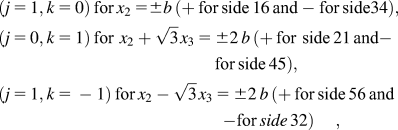
where the sides corresponding to the plus sign on the right side of the above equations are considered as the images of the ones corresponding to the minus sign under the transformations.
The macroscopic temperature gradients are defined as

where T 0 is the macroscopic temperature field. Equation (4) leads to the following relations between the macroscopic temperature gradients and the relative temperatures between corresponding points in different unit cells as origin and image,

where quantities with a prime are associated with the image point.
Substituting the coordinate relations in Eq. (2) into Eq. (5), the temperatures at  in the image cell H ’and those at P(x 2,x 3) in the unit cell H are related as follows:

Substituting the j and k values in Eq. (3) into Eq. (6), for a steady-state heat transfer problem using finite element analyses to calculate all effective thermal conductivities in the 2–3 plane, the temperature boundary conditions on the three paired sides can be obtained in the form of equations as, corresponding to (j = 1, k = 0), (j = 0, k = 1), and (j = 1, k = −1), respectively,

where notations  and
 , etc., inside the brackets indicate the sides while
 , etc., outside the brackets indicate the common coordinates shared by the corresponding points on the pair of sides.
The temperature boundary conditions for the unit cell have been defined previously on the six sides of the unit cell that are all in the form of equations. When these equation boundary conditions are discretized in finite element analyses, at the corners they are not independent because a corner is shared by two intersecting sides belonging to two different equations. Although incorporating these boundary conditions in finite element analyses does not introduce conflicts in a mathematical sense, some commercial finite element codes, e.g., ABAQUS, may diagnose it as a source of errors when this kind of equation boundary condition is imposed.12 To obtain independent equation boundary conditions at the corners, all corners are not included in equation boundary conditions, [Eq. (7)] for finite element analyses. They are considered separately as below. The six corners of the hexagonal unit cell can be classified into two groups, corners 1, 3, 5, and 2, 4, 6, as shown in Fig. 1(b). It is obvious that with any translational symmetry transformation the corners are transformed within a group but never from one group to another. Any one corner from each group can be selected as a reference corner because all the others from each group are related to this corner by certain translational symmetry transformation. Here, corner 1 from the first group and 6 from the second group are selected for example. Corners 3 and 5 are associated with corner 1 by translational symmetry transformations (j = 1, k = 0) and (j = 0, k = 1), respectively. Similarly, corners 2 and 4 are associated with corner 6 by translational symmetry transformations (j = 1, k = −1) and (j = 1, k = 0), respectively. Thus, the temperatures at these corners are related as follows:

where the subscripts to the temperatures indicate the corresponding corner numbers, as shown in Fig. 1(b).
To summarize, the temperature boundary conditions on the sides of the unit cell excluding corners are given in Eq. (7), those at the corners are given in Eq. (8). Applying these periodic boundary conditions, heat transfer analyses on this unit cell for a yarn can be performed. Concentrated heat fluxes can be applied to the unit cell through the extra degrees of freedom as will be discussed in the subsequent section.
B. Unit Cell 2—A cuboid
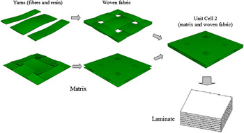
In real applications of composite materials, there are usually a significant number of layers of woven fabric stacked together to build up the desirable thickness. For the pattern of plain weave, all layers can be assumed to be identical and each of them can be reproduced by another by a simple translation. It is therefore sufficient to analyze a single layer. The regular woven pattern justifies the use of a unit cell to represent the layer. The unit cell involved here is referred to as Unit Cell 2 as shown in Fig. 2, which is a cuboid and contains matrix and woven yarns, warp and fill, each of which runs over one full period of undulation. The unit cell obtained from Voronoi tessellations can be described as domain enclosed by bisecting planes of the segment connecting the center of the unit cell and those of the neighboring cells. All Voronoi cells are identical throughout the space and any one cell can be reproduced by another through a certain translational symmetry transformation. The boundary of the unit cell as obtained from Voronoi tessellations consists of three paired faces, referred to as faces of the cell,

Schematic construction of Unit Cell 2, which represents a woven fabric laminate.

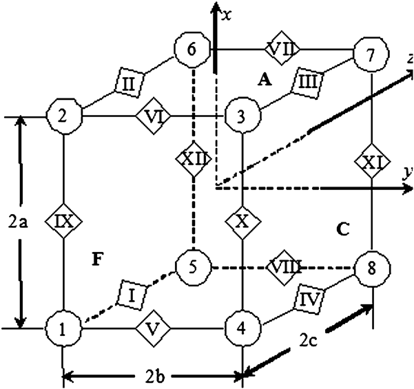
where a, b, and c are the dimensions of the unit cell as indicated in Fig. 3. The volume of the unit cell is V = 8 abc.
Unit Cell 2: cuboid and its faces, edges, and vertices.
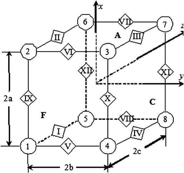
After the woven fabric composite has been tessellated into Voronoi cells, any Voronoi cell can be obtained from another Voronoi cell by certain translations in the x, y, and z directions. Under these translational symmetries, any point P(x′,y′,z′) in the material outside of the unit cell can be found as the image of a certain point P(x,y,z) in the unit cell under a translational symmetry transformation consisting of up to three translations in the x, y, and z directions. The coordinates of these two points are related as follows:

where i, j, k = 0, ±1, ±2,… are the numbers of Voronoi cells by which P′(x′,y′,z′) is away from P(x,y,z) in the x, y, and z directions, respectively. In this way, a set of three integer numbers, i, j, and k, defines uniquely a translational symmetry transformation. Substituting the coordinate relations in Eq. (10) into Eq. (5), one obtains

With translational symmetry transformations, the two faces in each of the three paired faces of the unit cell are transformed from one to another through the following transformations,

The faces corresponding to the plus sign on the right sides of the above equations are the images of the ones corresponding to the minus sign under the transformations. The three visible faces, A, C, and F are shown in Fig. 3 while the hidden counterparts are not shown to keep the sketch tidy, but they can be easily identified. Substituting these i, j, and k values in Eq. (12) into Eq. (11), the temperature boundary conditions on the three paired faces can be obtained in the form of equations as,

where notations |x =a and |x =−a, etc., inside the brackets indicate the faces while |y ,z, etc., outside the brackets indicate the common coordinates shared by the corresponding points on the pair of faces.
Similar to the Unit Cell 1, to obtain independent boundary conditions, all edges should be excluded from the temperature boundary conditions [Eq. (13)] on the faces of the unit cell because an edge is shared by two intersecting faces belonging to two different equations. The edges of the unit cell are numbered in Roman enclosed in diamond boxes, as shown in Fig. 3. The twelve edges of the unit cell can be classified into three groups, edges (IX, X, XI, and XII) parallel to the x axis, edges (V, VI, VII, and VIII) parallel to the y axis, and edges (I, II, III, and IV) parallel to the z axis, as shown in Fig. 3. It is obvious that with any translational symmetry transformation the edges are transformed within a group but never from one group to another. Any one edge from each group can be selected as a reference edge because all the others from each group are related to this edge by certain translational symmetry transformation. Here, for the group of edges parallel to the z axis, edge I is selected for example. Edges II, III, and IV are associated with edge I by translational symmetry transformations (i = 1, j = 0, k = 0), (i = 1, j = 1, k = 0) and (i = 0, j = 1, k = 0), respectively. For the other two groups of edges parallel to the x and y axis, they have similar transformations. Thus, the temperatures at these edges are related as follows:

where subscripts to the temperatures indicate the corresponding edge numbers as shown in Fig. 3. All vertices should be excluded from the temperature boundary conditions [Eq. (14)] on the edges of the unit cell because a vertex is shared by three intersecting edges belonging to three different equations. The vertices of the unit cell are numbered in Arabic enclosed in circles as shown in Fig. 3. Any vertex can be selected as a reference vertex because all the others are related to this vertex by certain translational symmetry transformation. Here, vertex 1 is selected for example. Vertex 7 is associated with vertex 1 by translational symmetry transformation (i = 1, j = 1, k = 1). For the other vertices, they have similar transformations. Thus, the temperatures at these corners are related as follows:

where the subscripts to the temperatures indicate the corresponding vertex numbers, as shown in Fig. 3.
To summarize, the temperature boundary conditions on the faces of the unit cell excluding edges are given in Eq. (13), those at the edges excluding vertices are given in Eq. (14), and for the vertices they are given in Eq. (15). Applying these boundary conditions, heat transfer analyses on this unit cell for the woven fabric composites can be performed via 3D finite element analyses. Concentrated heat fluxes can be applied to the unit cell through the extra degrees of freedom as will be discussed in the subsequent section.
C. Application of concentrated heat fluxes and effective thermal conductivities
Because the effective thermal conductivity is defined as the ratio of heat flux and temperature gradient, it is desired that either heat fluxes or temperatures are treated as the boundary conditions while the remainder will be considered as the responses. The macroscopic temperature gradients  ,
 or
 (
 ,
 , or
 in Unit Cell 1) can be treated as key/extra degrees of freedom to the system after incorporating equation boundary conditions in finite element analyses. In an actual finite element model, they can be assigned additional node numbers as ordinary nodes but with only one degree of freedom for each of such additional nodes or a single additional node with three degrees of freedom. After calculating by finite element analyses, corresponding heat fluxes can be obtained at these extra independent degrees of freedom. Alternatively, concentrated heat fluxes, Φx, Φy, or Φz, can also be applied to these key degrees of freedom. After calculating by finite element analyses, corresponding temperatures can be obtained at these additional independent degrees of freedom. The effective thermal conductivities of a unit cell can be obtained by the two equivalent ways. Heat fluxes are related to the concentrated heat fluxes as follows:

where V is the volume of the unit cell. In the case of Unit Cell 1, volume V is replaced by the area A of the unit cell as a unit length is assumed in the third dimension and coordinates x, y, and z are replaced by 1, 2, and 3.
The effective thermal conductivities of the composite represented by the unit cell concerned can be obtained as follows:

In UD fiber-reinforced composites as represented by Unit Cell 1, because materials properties do not vary in the longitudinal direction, the longitudinal thermal conductivity k 1 in the fiber’s direction can be obtained exactly from the rule of mixtures according to the definition of thermal conductivity coefficient in this direction

where κf and κm are the thermal conductivity of fiber and matrix, respectively.
In the presence of material symmetries, some of the effective thermal conductivities are equal. Calculating them individually and finding out whether these properties resulting from the symmetry considerations are observed properly can serve as good checks on the correct application of all the boundary conditions to the unit cell. In the finite element analysis, the actual magnitude of heat fluxes, including concentrated heat fluxes Φx, Φy, and Φz, would not affect the value of effective properties evaluated, as long as the system behaves linearly.
III. APPLICATIONS USING FINITE ELEMENTS: MESHING AND MATERIAL PROPERTIES
A. Finite element meshes
For all unit cells, commercial finite element codes PATRAN (MSC, 2005; MSC Software Corp., Los Angeles, CA) and ABAQUS 6.6-1 have been used for mesh generation and analysis, respectively. Meshes at different levels of refinement have been generated and they have been all analyzed to confirm the convergence of these meshes, i.e., further refinement would not result in any substantial improvement in the accuracy of the results. The boundary conditions in the form of equations for all these unit cells have been implemented using the “EQUATION” option in ABAQUS.12 To keep the corresponding nodes paired according to the relevant translational symmetries, the node numbers in the corresponding node sets need to be sorted properly. To achieve this goal, a small FORTRAN (The Fortran Company, Tucson, AZ) program suffices.
For Unit Cell 1, fiber is assumed to be of circular cross-section and perfectly bonded to matrix. It is reasonable to assume both fiber and matrix to be homogeneous and isotropic individually. Different fiber volume fractions from 0% to 85% will be considered. The mesh for the hexagonal unit cell at 60% of fiber volume fraction is shown in Fig. 1(a) as an example. Eight-node quadrilateral elements are used for generating the meshes for the fiber and matrix. The numerical analyses are carried out on a glass-fiber-reinforced epoxy resin matrix composite. The thermal conductivities for the fiber and resin as input data for Unit Cell 1 are 13 and 0.1 W/mK, respectively.
For Unit Cell 2, the bonding between yarns and resin is assumed to be perfect. The three dimensions of the unit cell obtained from scanning electron microscope (SEM) analyses are a = 3.05 mm, b = 3.05 mm, and c = 0.19 mm. It is assumed that the axes of warp yarns and fill yarns are described as the following cosine functions:

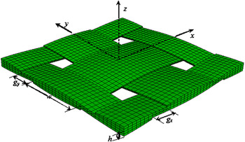
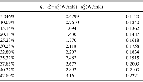
The cross section of yarns is assumed to be defined by the same functions above but truncated at both ends as determined by the dimension w. For the present fabric, it is assumed w = 2.38 mm and h = 0.16 mm and the spacing between two neighboring warp yarns or fill yarns is gx = gy = 0.67 mm, where parameters w, h, gx, and gy are as indicated in Fig. 4 and all obtained from SEM analyses. The z axis is in the thickness direction of the woven fabric composite. The volume fraction of the woven yarns in the Unit Cell 2 is 50.46%. Multiplying the volume fraction of the woven yarns by fiber volume fraction of Unit Cell 1, the overall fiber volume fraction in the composite can be obtained, which varies from 0% to 42.89%. For the yarns, the input data of thermal conductivities are the three thermal conductivities obtained from Unit Cell 1.
Parameters of woven yarns obtained from SEM analyses.

B. Coordinate transformation
The material for the yarns as represented by Unit Cell 1 is orthotropic. The three effective thermal conductivities ( ,
 , and
 ) of the yarns are given in the material’s principal axes. They are the input parameters required by Unit Cell 2. Because of the undulations in fill and warp yarns, the material’s principal axes vary along the axes of yarns within Unit Cell 2. To formulate the finite element model for Unit Cell 2, for the material representing the yarns in Unit Cell 2, coordination transformations have to be made from the material’s principal axes 1-2-3 to the global axes x-y-z. Because the orientation of material’s principal axes vary from point to point, the coordinate transformation matrix has to be defined point by point. The way to achieve this in ABAQUS12 is to use a user-defined orientation subroutine, “ORIENT,” in which the coordinate transformation matrix can be defined according to the spatial location of the point of interest. The detailed coordinate transformation can be found in Ref. 4.
IV. RESULTS AND DISCUSSION
After application of boundary conditions, some sanity checks have been made to the unit cells by setting the properties of the fiber or yarn the same as those of the matrix and carrying out analyses out of which exactly uniform heat flux distributions in the unit cells are obtained and all the calculated effective thermal conductivities are identical to the input value. These checks are essential because most errors resulting from formulation and node set can be eliminated. These have been carried out for all unit cells used in this study.
A. Effects of fiber volume fractions on the effective thermal conductivities of a yarn and comparison with the rule of mixtures
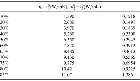
The effective thermal conductivities of a yarn are predicted using Unit Cell 1 for a range of fiber volume fractions, as listed in Table I. The lower and upper bounds of the effective thermal conductivities, according to the rule of mixtures, are given as

Effective thermal conductivities of a yarn predicted by the Unit Cell 1.
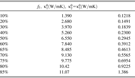
The effective thermal conductivities of a yarn predicted using Unit Cell 1 is shown in Fig. 5 along with their upper and lower bounds calculated from Eq. (20). To keep all the curves on one graph, the curves for  and lower bound have been magnified by one order of magnitude, i.e., the actual value of
 and lower bound obtained from the graph should be divided by 10. It can be seen from Fig. 5 that, with the increase of the fiber volume fraction, the
 increases linearly. The longitudinal thermal conductivity
 calculated from Eq. (18) is equal to the upper bound
 because they share the same formula. The transverse thermal conductivity
 increases with the fiber volume fraction monotonically with an increasing rate. Although the trend of variation is picked up by the lower bound, the actual values are significantly underestimated by the lower bound. The results of numerical analyses for the effective thermal conductivities of a yarn against results calculated by the rule of the mixtures indicate that although the rule of the mixtures gives accurate results for longitudinal thermal conductivity in the fiber direction, the rule of the mixtures gives inaccurate results for transverse thermal conductivities.
Effective thermal conductivities of a yarn predicted from Unit Cell 1 along with those calculated from the rule of mixtures.

B. Effects of fiber volume fractions on the effective thermal conductivities of the woven fabric composite
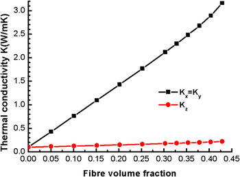
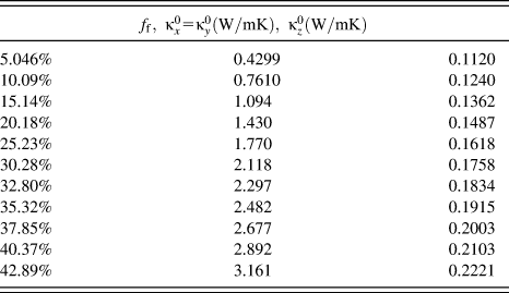
The effective thermal conductivities of the glass fiber woven fabric epoxy resin composite for different fiber volume fractions predicted from Unit Cell 2 are listed in Table II and charted in Fig. 6. The in-plane thermal conductivity is much higher than the transverse counterpart as shown in Fig. 6, which is obvious given the fact that fibers are mainly oriented along the plane of the fabric. The increasing rate of the in-plane thermal conductivities with the fiber volume fraction is much more sensitive than that of the transverse one.
Effective thermal conductivities of the glass fiber woven fabric epoxy resin composite predicted from Unit Cell 2.

Effective thermal conductivities of a composite predicted by the Unit Cell 2.
C. Heat flux distributions in the composite represented by Unit Cell 2
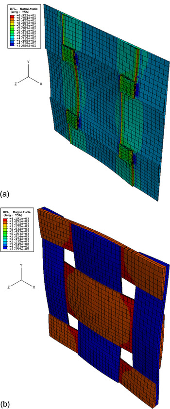
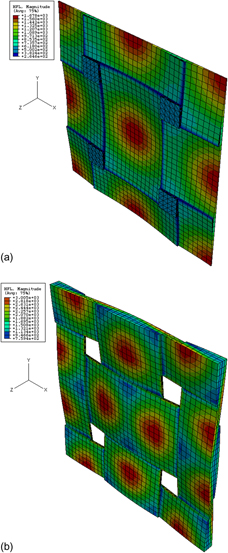
The heat flux distributions in Unit Cell 2, at a fiber volume fraction of 30.28%, loaded with concentrated heat flux Φx = 1 KW, are shown in Fig. 7. It can be seen from Fig. 7(b) that high values of heat fluxes are mostly found in the warp yarns, indicating that warp yarns are the main component of bearing heat in this loading case. The heat flux concentrations are mainly located at the intersection of warp and fill yarns and in the surrounding matrix. The areas where heat flux concentrations are most conspicuous are located around the intersections (a profile perpendicular to the heat transfer direction) where warp yarns meet the fill yarns. The maximum values of the heat flux are found to be 69.65 W/m2 in the matrix and 4191 W/m2 in the warp yarns, respectively.
Heat flux distributions in Unit Cell 2 with fiber volume fraction 30.28% under Φx = 1 KW: (a) sectioned view of the resin part and (b) woven yarns.

Figure 8 shows the heat flux distributions in Unit Cell 2 loaded with concentrated heat flux Φz = 1 KW. The areas of heat flux concentrations are a circular zone in the matrix against the tops of the humps of the undulating yarns and two elliptic zones in the woven yarns near the tops. The maximum values of the heat flux are 1678 W/m2 in the matrix and 3005 W/m2 in the yarns, respectively. The heat flux in the matrix is much higher than the counterpart under in-plane loading, which indicates that the matrix loaded under transversely concentrated heat flux, is easily subjected to fire damage.
Heat flux distributions in Unit Cell 2 with fiber volume fraction 30.28% under Φz = 1 KW: (a) sectioned view of the resin part and (b) woven yarns.

D. Parametric studies
Thermal conductivities of the composite caused by the variation of the constituent materials cannot be measured easily. A sensitivity study is therefore required. The parametric study was based on the plain weave glass fabric reinforced epoxy resin matrix composite as analyzed previously in this work. Figure 9 shows the effective thermal conductivities of the composite versus fiber volume fraction with the thermal conductivity of resin increasing from 0.1 to 0.4 W/mK, while the thermal conductivity of fiber remains at 13 W/mK. It can be seen from this figure that with the increase of the thermal conductivity of resin, all effective thermal conductivities of the composite increase proportionally. The variations of these properties with fiber volume fraction have been discussed previously.
Effects of variation of the thermal conductivity of resin on the variation of effective thermal conductivities of the composite.

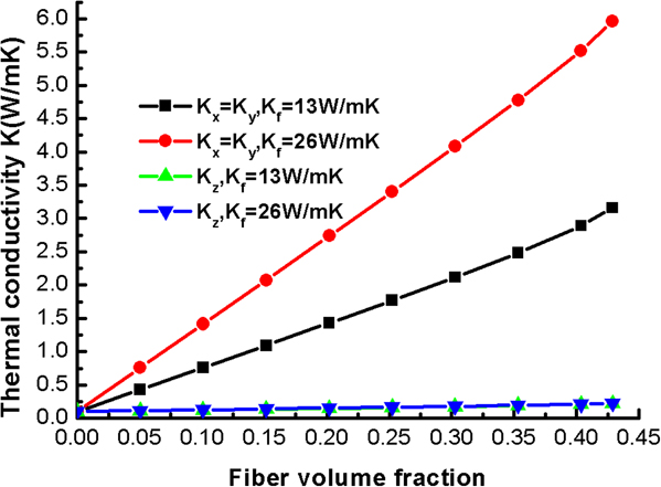
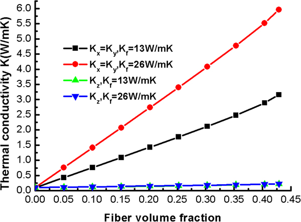
The curves of the effective thermal conductivities of the composite versus fiber volume fraction are plotted in Fig. 10 with the thermal conductivity of fiber increasing from 13 to 26 W/mK, while the thermal conductivity of resin remains at 0.1 W/mK. The influence of the variation of the thermal conductivity of fiber on transverse thermal conductivity is nearly unnoticeable, while its influence on in-plane thermal conductivities is pronounced.
Effects of variation of the thermal conductivity of fiber on the variation of effective thermal conductivities of the composite.
V. SUMMARY
This work presents a numerical approach to predict the effective thermal conductivities of woven fabric composites. The representative volume element method based on the assumption of periodic distribution of the fibers in the yarns and periodic arrangement of the reinforcing yarns in the woven fabric composites has been used to facilitate the finite element analyses. The industrial designers can easily adopt similar procedures to study and optimize composite materials varying the factors (such as weave style) that affect their mechanical and thermal properties.
ACKNOWLEDGMENTS
The work as published in this paper was jointly funded by the Engineering and Physical Science Research Council (EPSRC) under Grant No. EP/D000734/1 and the Ministry of Defense under the Joint Grant Scheme (Dstl/06/JGS/998,999).