1. Introduction
The recent development of micro-fluidic based devices has pushed the scientific community to reconsider classical issues in fluid dynamics such as the hydrodynamical behaviour of micro-scale bodies in the creeping regime. For instance, propulsion of microswimmers, see e.g. Fauci & Dillon (Reference Fauci and Dillon2006), Lauga & Powers (Reference Lauga and Powers2009), Guasto, Rusconi & Stocker (Reference Guasto, Rusconi and Stocker2012), Elgeti, Winkler & Gompper (Reference Elgeti, Winkler and Gompper2014), has been addressed for the production of energy oriented to micro-devices (Di Leonardo et al. Reference Di Leonardo, Angelani, Dell Arciprete, Ruocco, Iebba, Schippa, Conte, Mecarini, De Angelis and Di Fabrizio2010; Sokolov et al. Reference Sokolov, Apodaca, Grzybowski and Aranson2010) and for the self-propulsion of micro-robots (Pak et al. Reference Pak, Zhu, Brandt and Lauga2012; Alouges et al. Reference Alouges, De Simone, Heltai, Lefebvre-Lepot and Merlet2013). The microswimmer’s behaviour in the presence of confining surfaces is also crucial for biofilm formation. Most studies (Pratt & Kolter Reference Pratt and Kolter1998; Rusconi et al. Reference Rusconi, Lecuyer, Guglielmini and Stone2010) focused on the biofilm formation at solid–liquid interfaces. Biofilm formation near air–liquid interfaces is also a problem of significant concern, since the liquid–air biofilm can be advantageous for aerobic micro-organisms, providing them access to oxygen (from the air) and nutrients (from the liquid) at the same time (Constantin Reference Constantin2009; Koza et al. Reference Koza, Hallett, Moon and Spiers2009). Several species of flagellated bacteria are known to form biofilms at liquid–air interfaces, e.g. Bacillus subtilis, Bacillus cereus and Pseudomonas fluorescens. For instance, the preparation of the well-known Natto from Japanese cooking, consisting of fermented soy beans, involves B. subtilis in significant concentrations (Chantawannakul et al. Reference Chantawannakul, Oncharoen, Klanbut, Chukeatirote and Lumyong2002). In contrast, some strains of B. cereus are known to be harmful to humans and cause foodborne illness (Ehling-Schulz, Fricker & Scherer Reference Ehling-Schulz, Fricker and Scherer2004). P. fluorescens, instead, is able to contaminate heparinized saline flushes used in cancer therapy (Gershman et al. Reference Gershman, Kennedy, Noble-Wang, Kim, Gullion, Kacica, Jensen, Pascoe, Saiman and McHale2008). Despite its biological implications, the mechanics of flagellated swimmers close to a liquid–air interface is much less explored than the case of a liquid–solid interface.
At micro-scales viscous effects overwhelm inertia leading to the development of apparently counterintuitive swimming strategies as proved by the Scallop theorem (Purcell Reference Purcell1977; Lauga Reference Lauga2011). In a nutshell, if the swimmer deforms through a sequence of body configurations which are periodic and time-reversible (reciprocal motion), its average motion is zero. The reciprocal motion can be exploited for locomotion only when nonlinear or memory effects are relevant. Examples are the non-Newtonian behaviour of the fluid (Lauga Reference Lauga2009; Keim, Garcia & Arratia Reference Keim, Garcia and Arratia2012; Qiu et al. Reference Qiu, Lee, Mark, Morozov, Münster, Mierka, Turek, Leshansky and Fischer2014) or motions occurring close to deformable interfaces (Trouilloud et al. Reference Trouilloud, Tony, Hosoi and Lauga2008). Micro-organisms developed many different strategies based on nonreciprocal effects to overcome the above restrictions. The Spiroplasma deforms its cytoskeleton by propagating pairs of kinks (Trachtenberg, Gilad & Geffen Reference Trachtenberg, Gilad and Geffen2003; Yang, Wolgemuth & Huber Reference Yang, Wolgemuth and Huber2009). Other microswimmers exploit their cilia wavy motion (Maxey Reference Maxey2011) as done by Paramecium (Jana, Um & Jung Reference Jana, Um and Jung2012).
However, many micro-organisms take advantage of single or multiple flagella, such as the Caulobacter crescentus, which has a single (right-handed) helical filament driven by a rotary motor (Li & Tang Reference Li and Tang2006) and the E. coli that has multiple flagella (Berg Reference Berg2004). The flagellar motor which activates and controls the filament rotation is able to switch between both rotation directions (Wang, Yuan & Berg Reference Wang, Yuan and Berg2014), and, as a first approximation, the torque applied to the filament is constant (Berg Reference Berg2004). In the case of the E. coli the flagella arrange in a bundle, characterized by a left-handed rotation of the motor which confers to bacteria a smooth forward motion (run phase). The flagella is also able to invert the rotation direction in order to let the bacteria at rest and change its direction (tumble phase). Due to their internal structure, the filaments can only assume twelve prescribed shapes (helical polymorphic states) but only one of those is the ‘normal state’, i.e. it is the most observed one during the run phase (Darnton & Berg Reference Darnton and Berg2007; Vogel & Stark Reference Vogel and Stark2010). Hence, the flagella can be modelled as a rigid single filament (Phan-Thien, Tran-Cong & Ramia Reference Phan-Thien, Tran-Cong and Ramia1987; Shum, Gaffney & Smith Reference Shum, Gaffney and Smith2010) rotating around the bacterial head axis.
The main purpose of this work is an extensive analysis of the hydrodynamical behaviour of a flagellated microswimmer close to air–liquid interfaces, with particular attention to free surfaces. For the sake of definiteness, we focus on a simplified geometry modelling the configuration of E. coli whose swimming is probably the most widely studied from both experimental and numerical points of view. Anyhow, in order to explore the effect of different geometrical parameters, several modified configurations are also discussed.
Flagellated swimmers close to a free surface have already been addressed by simplified models, see e.g. Crowdy et al. (Reference Crowdy, Lee, Samson, Lauga and Hosoi2011), Di Leonardo et al. (Reference Di Leonardo, Dell Arciprete, Angelani and Iebba2011), Lopez & Lauga (Reference Lopez and Lauga2014) where two-dimensionality, resistive force theory, and multipole expansions techniques were exploited, respectively. To the best of our knowledge, the present work addresses the first fully three-dimensional numerical simulation of a swimmer in the presence of an liquid–air interface. Given the linearity of the Stokes equations, which are the appropriate model for creeping flows, the numerical approach exploits the boundary element method (BEM). The BEM can easily handle the complex geometry of the microswimmer and account for different boundary conditions. Moreover, a flat and infinitely extended free surface and/or solid wall (when needed for comparisons) can be easily included by considering the appropriate Green’s function, thus avoiding any undesired effect of the numerical truncation of the domain.
There is a wide body of literature available dealing with the motion of micro-organisms in free space or close to solid boundaries. Since the first studies by Taylor (Reference Taylor1951), attention has principally focused on micro-organisms whose flagellum was modelled as an infinite cylindrical filament in an unbounded fluid endowed with small-amplitude wavy motion. In fact, it was initially believed that the flagella were only moved by wave propagation. However Berg & Anderson (Reference Berg and Anderson1973) showed that bacteria could also rotate their flagella in a corkscrew-like motion, moving the flagellar bundle as a single filament. The flagellum has a large aspect ratio, with length exceeding thickness by more than two orders of magnitude (Lauga & Powers Reference Lauga and Powers2009). This particular geometry pushed the adoption of a Slender Body Theory (SBT) that has been exploited in several studies to evaluate the translational velocity and/or the torque applied by the swimmer (Hancock Reference Hancock1953). Successively (Higdon Reference Higdon1979a ,Reference Higdon b ) transformed the Stokes equations into a system of singular integral equations accounting for the swimmer translational and angular velocities. He added to the SBT a variable strength of the singularity along the flagellum centreline, thus modelling different centreline geometries. In this case, both the planar sinusoidal motion and the rotation about the body axis were amenable to modelling. By an appropriate system of images, the SBT could also account for a spherical cell body and the presence of a wall. However too many restrictions still confined the SBT application to extremely simplified configurations.
In recent years the increase of computational resources has led to a more extensive use of the BEM which overcomes many drawbacks of the SBT in dealing with microswimmers both in free space and confined conditions. Phan-Thien et al. (Reference Phan-Thien, Tran-Cong and Ramia1987) used the BEM to study the motion of a micro-organism in free space. Successively, Ramia, Tullock & Phan-Thien (Reference Ramia, Tullock and Phan-Thien1993) applied the BEM to the interaction between the swimmer and a solid wall, showing that when swimming close to a solid wall, the swimmer exhibited a circular motion. The BEM was also used to study the interactions between two neighbouring flagellated microswimmers, highlighting the possibility of a coordination between their flagellar motion in order to maximize their velocities (Ramia et al. Reference Ramia, Tullock and Phan-Thien1993).
More recently, Lauga et al. (Reference Lauga, DiLuzio, Whitesides and Stone2006) experimentally investigated the motion of an E. coli near a solid wall and found, as predicted by Ramia et al. (Reference Ramia, Tullock and Phan-Thien1993), a circular clockwise motion. In the paper the authors also provided a simple theoretical model which was able to explain their experimental observations. Interestingly, the same model suggested that the bacteria should reverse its rotation when swimming in the proximity of a free surface. The same authors also showed that the swimmer is attracted by a solid wall. This behaviour was investigated in detail a few years later by Giacché, Ishikawa & Yamaguchi (Reference Giacché, Ishikawa and Yamaguchi2010) in a numerical work which highlighted how the bacteria could move at a stable distance from a wall. At the same time Shum et al. (Reference Shum, Gaffney and Smith2010) investigated the motion of a microswimmer close to solid walls by considering many geometrical configurations and relating the shape of the body to the propulsion efficiency and to the possibility of achieving different motions, i.e. to be attracted by the wall, to escape from the wall or to reach stable circular orbits at a given wall-normal distance. The same authors (Shum & Gaffney Reference Shum and Gaffney2012) also focused on the flexible hooks linking each flagellum to the cell. They studied the modifications in the microswimmer trajectories when changing the hook rigidities. They found that, within an intermediate range of rigidities, the swimmer behaviour does not change too much with respect to the simpler model of rigid hook. The same work highlighted how, for particular values of relative hook stiffness, there is a transient phase of periodic motion with constant average distance from the wall, leading to boundary accumulation. The tendency of swimming micro-organisms to accumulate near solid walls (Li & Tang Reference Li and Tang2009), with particular emphasis on collisions with the surface and rotational Brownian motion, has also been investigated and linked to the swimming speed and the cell size (Li et al. Reference Li, Bensson, Nisimova, Munger, Mahautmr, Tang, Maxey and Brun2011) of the microswimmer. Recent works extended the investigation about the motion of microswimmers to more complex surfaces: a clean fluid–fluid interface, a slipping rigid wall and a fluid interface covered by surfactants (Lopez & Lauga Reference Lopez and Lauga2014). The authors used an asymptotic, far-field approximation to represent the actual swimmer, retaining information about velocities and rotations. The case of two fluid interfaces, in the limit of vanishing viscosity of one of them, allowed for a description of a free surface. In such conditions, the swimmer exhibited counter-clockwise motion. This confirmed the results anticipated by Lauga et al. (Reference Lauga, DiLuzio, Whitesides and Stone2006). Also Di Leonardo et al. (Reference Di Leonardo, Dell Arciprete, Angelani and Iebba2011) supported by means of experimental observations the theoretical prediction made through a simplified model based on the method of images and the resistive force theory. Even if neglecting all the dynamics of the swimmer outside the interface plane, this work provided a simple explanation for a counter-clockwise motion over a perfectly slipping surface, showing a good agreement between the results of the simplified model and the experimental observation. Briefly, Lauga et al. (Reference Lauga, DiLuzio, Whitesides and Stone2006) explain that, when swimming above a no-slip surface, a positive rotation rate of the swimmer head around its longitudinal axis produces a lateral force which is opposite to the one induced by the negative tail rotation rate. As a consequence, a net torque normal to the wall is exerted on the body such that the swimmer follows a clockwise (CW) trajectory. Otherwise, when swimming close to a liquid–air interface, Di Leonardo et al. (Reference Di Leonardo, Dell Arciprete, Angelani and Iebba2011) devise a simplified model based on resistive force theory endowed with suitable symmetries to satisfy the free-slip condition at the interface. In this model, the swimmer moves under the effect of the velocity generated by its mirror image below the interface. The counter-rotating image head produces on the swimmer head a lateral velocity which is opposite to the force that is exerted in the case of a solid wall. Such relative velocity gives rise to a corresponding viscous force in the same direction. Since the same reasoning applies to the counter rotating tail, the overall torque on the microswimmer is also opposite to the one experienced on a no-slip wall, hence a net CCW motion is produced. In literature a clockwise motion has been observed (Lemelle et al. Reference Lemelle, Palierne, Chatre and Place2010) also in presence of a free surface. Based on experimental observations, Morse et al. (Reference Morse, Huang, Li, Maxey and Tang2013) attributed such a behaviour to molecular adsorption (due to the presence of biological material in the growth medium) altering the rheological properties of the air–water interface, thus determining the swimming pattern of nearby cells.
In principle, the mechanical causes that can affect the swimming direction are: (i) the rotation direction of the flagellum bundle; (ii) the effective boundary condition at the planar surface. This study focuses on the point (ii) through the numerical simulation of the motion of a E. coli-like microswimmer close to free-slip and no-slip surfaces, assuming a standard left-handed arrangement for the flagellum bundle. The aim is to investigate the behaviour of the swimmer by addressing in full detail the complete three-dimensional nature of the hydrodynamical interaction between the swimmer and the surface. It is worth noting that free slip and no slip are the limits of the more general Navier boundary condition that connects the velocity at the liquid boundary with the tangential stress (Bazant & Vinogradova Reference Bazant and Vinogradova2008). For liquid water moving on a solid surface, the actual slip is negligible at the micro-scale also for hydrophobic coatings (Chinappi & Casciola Reference Chinappi and Casciola2010; Sega et al. Reference Sega, Sbragaglia, Biferale and Succi2013) and only the presence of vapour bubbles trapped in the surface asperities (superhydrophobic surfaces) leads to significant slippage (Bolognesi et al. Reference Bolognesi, Cottin-Bizonne, Guene, Teisseire and Pirat2013; Gentili et al. Reference Gentili, Bolognesi, Giacomello, Chinappi and Casciola2014), potentially altering the motion of particles close to the surface (Nizkaya et al. Reference Nizkaya, Asmolov, Zhou, Schmid and Vinogradova2014; Pimponi et al. Reference Pimponi, Chinappi, Gualtieri and Casciola2014). Hence, the no-slip boundary is, for the present purposes, a reliable model of a rigid wall. On the other hand, the proper boundary conditions at the liquid–air interface are impermeability and continuity of the tangential stress components, that reduce to free slip (zero tangential stress) since the air density is an order of magnitude smaller than the liquid one.
The paper is organized as follows: the geometrical model of the swimmer and the BEM are addressed in § 2. Section 3 reports the salient results concerning the motion of the swimmer in the presence of a free surface. Finally, we discuss the major findings and point out the main conclusions (§ 4), giving a perspective view of future work.
2. Boundary integral formulation for the microswimmer
2.1. Swimmer model
This section concerns the modelling of a microswimmer inspired by E. coli. This bacteria has been investigated at length in the literature and a lot of information about its geometry and propulsion mechanism is available. E. coli has a cell length which varies between
 $1.6$
and
 $3.9~{\rm\mu}\text{m}$
, the cell width ranges between
 $0.9$
and
 $1.7~{\rm\mu}\text{m}$
, with a resulting cell volume from
 $1.5$
to
 $4.4~{\rm\mu}\text{m}^{3}$
(Volkmer & Heinemann Reference Volkmer and Heinemann2011) and an average length of flagella of approximately
 $7~{\rm\mu}\text{m}$
(Lauga et al.
Reference Lauga, DiLuzio, Whitesides and Stone2006).
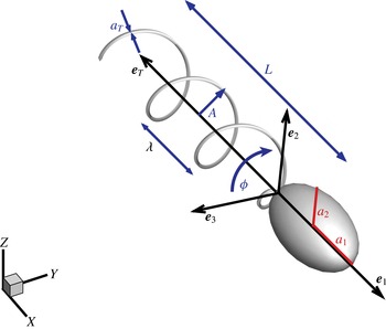
The model of the flagellated swimmer comprises an ellipsoidal head (cell) and a tubular, helical, rigid, tail (flagellum). The tail rotates about its axis
 $\boldsymbol{e}_{T}$
of an angle
 ${\it\phi}(t)$
. The dimensionless semi-axes of the head are
 $a_{1}$
and
 $a_{2}$
. The head aspect ratio is kept constant,
 $AR=a_{1}/a_{2}=2$
, and the equivalent radius (i.e. the radius
 $\bar{a}$
of a sphere with same volume) is the assumed reference length. The dimensionless tail length is
 $L=7$
, with a cross-section radius
 $a_{t}=0.05$
. The dimensionless helix amplitude and wavelength are
 $A$
and
 ${\it\lambda}$
, respectively.
 $\{\boldsymbol{e}_{1},\boldsymbol{e}_{2},\boldsymbol{e}_{3}\}$
are the orthonormal vectors of the frame attached to the swimmer head (body frame).
 $\boldsymbol{e}_{1}$
is longitudinal and identifies the swimmer orientation with respect to the unit vectors of the fixed frame
 $\{\boldsymbol{X},\boldsymbol{Y},\boldsymbol{Z}\}$
.

Figure 1 sketches the simplified geometry comprising the ellipsoidal axisymmetric cell and the corkscrew tail. Hereafter, the equivalent radius of the ellipsoidal cell
 $\bar{a}$
(the radius of the sphere having the same volume) will be used as reference length scale, i.e. the dimensionless cell volume is
 $V=3V^{\prime }/4{\rm\pi}\bar{a}^{3}=1$
, where the prime identifies dimensional quantities. The cell aspect ratio is
 $AR=a_{1}/a_{2}=2$
, with
 $2a_{1}$
and
 $2a_{2}$
the longitudinal and the transversal (dimensionless) axes. Following Shum et al. (Reference Shum, Gaffney and Smith2010), the tail bundle is modelled as a single helix with radius
 $a_{T}=0.05$
. The tail rotates around its axis
 $\boldsymbol{e}_{T}$
(see figure 1). The dimensionless axial length of the helix is
 $L$
,
 $A$
denotes the helix amplitude and
 ${\it\lambda}$
its wavelength. In the present work we selected typical values for the tail length and cell axes, namely
 $L=7$
,
 $a_{1}=1.6$
and
 $a_{2}=0.8$
, while the amplitude
 $A$
and the wavelength
 ${\it\lambda}$
of the tail are systematically varied. With the above choices, the swimmer is rescaled into an actual E. coli by assuming
 $\bar{a}=1~{\rm\mu}\text{m}$
.
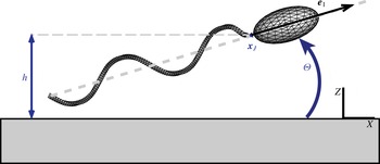
Sketch of the discretized swimmer near a planar surface. The configuration is identified by three parameters, namely, the distance
 $h$
of the reference point
 $\boldsymbol{x}_{J}$
from the plane and the pitch angle
 ${\it\Theta}$
. The third parameter is the tail rotation angle
 ${\it\phi}$
defined in figure 1.

It is useful to introduce a body reference frame with orthonormal base vectors
 $\{\boldsymbol{e}_{1},\boldsymbol{e}_{2},\boldsymbol{e}_{3}\}$
where
 $\boldsymbol{e}_{1}=-\boldsymbol{e}_{T}$
is longitudinal (see figure 1). The subscript
 $H$
identifies the head and the subscript
 $T$
refers to the tail, which can rotate with respect to the head about its axis
 $\boldsymbol{e}_{T}$
. During the tail rotation around
 $\boldsymbol{e}_{T}$
, each point of the rigid tail describes a circle in the plane normal to
 $\boldsymbol{e}_{T}$
, with
 ${\it\phi}$
the corresponding rotation angle (or flagellum phase). The time derivative
 $\dot{{\it\phi}}(t)$
is the tail rotational velocity
 ${\it\Omega}_{T}$
. The swimmer position is identified in a fixed reference frame with base
 $\{\boldsymbol{X},\boldsymbol{Y},\boldsymbol{Z}\}$
by the three coordinates of the cell-to-tail junction point
 $\boldsymbol{x}_{J}$
, see figure 2. The swimmer translates with dimensionless velocity
 $\boldsymbol{U}=\boldsymbol{U}^{\prime }/v$
and has angular velocity
 ${\it\bf\Omega}_{H}={\it\bf\Omega}_{H}^{\prime }\bar{a}/v$
, where
 $v\simeq 20~{\rm\mu}\text{m}~\text{s}^{-1}$
is a typical swimming velocity taken as a reference quantity. The
 $\{\boldsymbol{X},\boldsymbol{Y}\}$
coordinate plane is taken to coincide with the planar boundary, either the solid wall or the free surface, see figure 2.
The kinematics of the swimmer is described by seven degrees of freedom, the junction position
 $\boldsymbol{x}_{J}(t)$
, the flagellum phase
 ${\it\phi}(t)$
and the three parameters defining the rotation of the head. We stress that the discretely evolved rotation matrix should belong to the proper matrix subspace, namely the
 $\text{SO}(3)$
subgroup. This is enforced through a description in terms of quaternions with unit norm, see e.g. Diebel (Reference Diebel2006). It follows that
 $$\begin{eqnarray}\displaystyle & \displaystyle \dot{\boldsymbol{x}}_{J}=\boldsymbol{U}(t), & \displaystyle\end{eqnarray}$$
 $$\begin{eqnarray}\displaystyle & \displaystyle \dot{{\it\phi}}={\it\Omega}_{T}(t), & \displaystyle\end{eqnarray}$$
 $$\begin{eqnarray}\displaystyle & \displaystyle \dot{\boldsymbol{q}}={\textstyle \frac{1}{2}}\unicode[STIX]{x1D64E}(\boldsymbol{q}){\it\bf\Omega}_{H}(t), & \displaystyle\end{eqnarray}$$
 $\boldsymbol{q}=(q_{0},q_{1},q_{2},q_{3})$
is the quaternion vector with
 $|\boldsymbol{q}|=1$
. When
 ${\it\bf\Omega}_{H}(t)$
is expressed in the
 $\{\boldsymbol{X},\boldsymbol{Y},\boldsymbol{Z}\}$
base,
 $\unicode[STIX]{x1D64E}$
reads
 $$\begin{eqnarray}\unicode[STIX]{x1D64E}(\boldsymbol{q})=\left[\begin{array}{@{}rrr@{}}-q_{1} & -q_{2} & -q_{3}\\ q_{0} & -q_{3} & q_{2}\\ q_{3} & q_{0} & -q_{1}\\ -q_{2} & q_{1} & q_{0}\end{array}\right].\end{eqnarray}$$
Given the quaternion
 $\boldsymbol{q}(t)$
, the components of the body frame unit vectors can be reconstructed as
 $$\begin{eqnarray}\displaystyle \left.\begin{array}{@{}c@{}}\boldsymbol{e}_{1}=\left(q_{0}^{2}+q_{1}^{2}-q_{2}^{2}-q_{3}^{2},2(q_{1}q_{2}+q_{0}q_{3}),2(q_{1}q_{3}-q_{0}q_{2})\right),\\ \boldsymbol{e}_{2}=\left(2(q_{1}q_{2}-q_{0}q_{3}),q_{0}^{2}-q_{1}^{2}+q_{2}^{2}-q_{3}^{2},2(q_{2}q_{3}+q_{0}q_{1})\right),\\ \boldsymbol{e}_{3}=\left(2(q_{1}q_{3}+q_{0}q_{2}),2(q_{2}q_{3}-q_{0}q_{1}),q_{0}^{2}-q_{1}^{2}-q_{2}^{2}+q_{3}^{2}\right).\end{array}\right\} & & \displaystyle\end{eqnarray}$$
Time integration of (2.1)–(2.3), allows us to track the swimmer trajectory once
 $\boldsymbol{U}$
,
 ${\it\bf\Omega}_{H}$
and
 ${\it\Omega}_{T}$
are determined by the solution of the hydrodynamical interactions between the swimmer and the fluid, as discussed in the next section. Since the numerical integration error in the equations for the quaternion may affect its norm, the quaternion is normalized to unit length at each time step. It easily shown that the accuracy of the integration scheme is exactly preserved by this procedure.
2.2. Hydrodynamic model
Given the characteristic length scale
 $\bar{a}$
and swimming velocity
 $v$
of the micro-organism, the typical Reynolds number in water is
 $Re={\it\rho}\bar{a}v/{\it\mu}\simeq 2\times 10^{-5}$
where
 ${\it\mu}$
and
 ${\it\rho}$
are the water viscosity and density, respectively. Hence the inertial terms are negligible and, for Newtonian fluids, the flow in the domain
 $\mathscr{D}$
is described by the Stokes equations,
 $$\begin{eqnarray}\displaystyle & \displaystyle \boldsymbol{{\rm\nabla}}\boldsymbol{\cdot }\boldsymbol{u}=0, & \displaystyle\end{eqnarray}$$
 $$\begin{eqnarray}\displaystyle & \displaystyle {\rm\nabla}^{2}\boldsymbol{u}-\boldsymbol{{\rm\nabla}}p=0, & \displaystyle\end{eqnarray}$$
 $\boldsymbol{u}=\boldsymbol{u}^{\prime }/v$
and
 $p=p^{\prime }\bar{a}/({\it\mu}v)$
.
The flow velocity
 $\boldsymbol{u}$
is forced by the tension
 $\boldsymbol{f}$
at the swimmer surface acting on the fluid. The swimmer propulsion is due to the internal (constant) torque
 ${\it\tau}_{M}={\it\tau}_{M}^{\prime }/({\it\mu}v\bar{a}^{2})$
exchanged between head and tail. Being a free body, the total force and torque on the swimmer (head and tail) is zero,
 $$\begin{eqnarray}\displaystyle & \displaystyle \int _{H\cup T}\boldsymbol{f}\,\text{d}S=0, & \displaystyle\end{eqnarray}$$
 $$\begin{eqnarray}\displaystyle & \displaystyle \int _{H\cup T}\boldsymbol{r}\wedge \boldsymbol{f}\,\text{d}S=0, & \displaystyle\end{eqnarray}$$
 $\boldsymbol{r}=\boldsymbol{x}-\boldsymbol{x}_{J}$
. The torque
 ${\it\tau}_{M}$
exerted on the tail is balanced by the torque produced by the fluid stresses
 $\boldsymbol{f}$
on the tail boundary, namely
 $$\begin{eqnarray}\boldsymbol{e}_{T}\boldsymbol{\cdot }\int _{T}\boldsymbol{r}\wedge \boldsymbol{f}\,\text{d}S=-{\it\tau}_{M}.\end{eqnarray}$$
The system (2.6)–(2.8) needs proper boundary conditions at the swimmer surface and external boundaries, i.e. wall or free surface. On the microswimmer surface the no-slip condition yields
 $$\begin{eqnarray}\displaystyle \boldsymbol{u}(\boldsymbol{x})=\left\{\begin{array}{@{}ll@{}}\displaystyle \boldsymbol{U}+{\it\bf\Omega}_{H}\wedge \boldsymbol{r} & (\boldsymbol{x}\in H),\\ \displaystyle \boldsymbol{U}+({\it\bf\Omega}_{H}+{\it\Omega}_{T}\boldsymbol{e}_{T})\wedge \boldsymbol{r} & (\boldsymbol{x}\in T).\end{array}\right. & & \displaystyle\end{eqnarray}$$
A no-slip boundary condition is also used to model the solid wall. For the free surface, vanishing normal fluid velocity (impermeability) and zero tangential stresses (free-slip condition) are the appropriate prescriptions,
 $$\begin{eqnarray}\displaystyle & \displaystyle \boldsymbol{u}\boldsymbol{\cdot }\boldsymbol{n}=0, & \displaystyle\end{eqnarray}$$
 $$\begin{eqnarray}\displaystyle & \displaystyle \left(\left(\boldsymbol{{\rm\nabla}}\boldsymbol{u}+(\boldsymbol{{\rm\nabla}}\boldsymbol{u})^{\text{T}}\right)\boldsymbol{\cdot }\boldsymbol{n}\right)(\boldsymbol{I}-\boldsymbol{n}\otimes \boldsymbol{n})=0. & \displaystyle\end{eqnarray}$$
2.3. Boundary element method
The solution of the Stokes equations (2.6) can be recast in integral form
 $$\begin{eqnarray}E(\boldsymbol{x}_{0})\,u_{i}(\boldsymbol{x}_{0})=\int _{\partial \mathscr{D}}\left[u_{j}(\boldsymbol{x})\unicode[STIX]{x1D61B}_{ikj}(\boldsymbol{x},\boldsymbol{x}_{0})n_{k}(\boldsymbol{x})-\unicode[STIX]{x1D60E}_{ij}(\boldsymbol{x},\boldsymbol{x}_{0})f_{j}(\boldsymbol{x})\right]\text{d}S,\end{eqnarray}$$
where
 $E(\boldsymbol{x}_{0})=1$
for points belonging to the interior of the domain.
 $\unicode[STIX]{x1D60E}_{ij}(\boldsymbol{x},\boldsymbol{x}_{0})$
is the free-space Green function, i.e. the
 $i$
th component of the velocity at
 $\boldsymbol{x}$
induced by a Dirac
 ${\it\delta}$
-like force at
 $\boldsymbol{x}_{0}$
acting in direction
 $j$
, and
 $\unicode[STIX]{x1D61B}_{ikj}(\boldsymbol{x},\boldsymbol{x}_{0})$
the associated stress tensor (Happel & Brenner Reference Happel and Brenner1983). Equation (2.11) expresses the
 $i$
th velocity component at the collocation point
 $\boldsymbol{x}_{0}$
in the fluid domain
 $\mathscr{D}$
. It requires knowledge of the velocity
 $u_{j}(\boldsymbol{x})$
and the stresses
 $f_{j}(\boldsymbol{x})$
at the boundary
 $\partial \mathscr{D}$
. The integral representation (2.11) can be turned into a boundary integral equation in the limit
 $\boldsymbol{x}_{0}\rightarrow \partial \mathscr{D}$
. The resulting expression can be written in the same form (2.11) now with
 $E(\boldsymbol{x}_{0})=1/2$
and the integral understood in the Cauchy principal-value sense. We emphasize that the boundary
 $\partial \mathscr{D}$
consists of two disjointed parts: the swimmer surface and the planar interface. The integral can be restricted to the swimmer’s surface by exploiting the symmetries associated with the boundary condition at the planar interface. This is tantamount to the use of the appropriate Green’s function, see appendix A, for the free-slip case and Blake (Reference Blake1971) for the no-slip case.
Due to the boundary condition (2.9) the fluid velocity at the swimmer surface is expressed in terms of seven unknowns, namely, the velocity of the junction point
 $\boldsymbol{U}$
, the angular velocity
 ${\it\bf\Omega}_{H}$
and the tail rotation velocity
 ${\it\Omega}_{T}$
, which together with the tension
 $\boldsymbol{f}$
at the swimmer surface complete the set of unknowns. The system of equations consists of the vector boundary integral equation (2.11), the global force and torque balance (2.7) and the torque balance for the swimmer’s tail (2.8). It can be shown that the solution exists and is unique (Ladyzhenskaya & Silverman Reference Ladyzhenskaya and Silverman1969).
The above system is discretized by means of
 $N$
curved 6-point elements (typically
 $N=3518$
total elements, with
 $N_{H}=512$
panels on the swimmer head), as sketched in figure 2, with piecewise constant shape functions (Pozrikidis Reference Pozrikidis1992). By selecting the centre of each element as a collocation point
 $\boldsymbol{x}_{0}$
, the boundary integral equation (2.11) with
 $E(\boldsymbol{x}_{0})=1/2$
is recast in a system of
 $3N$
scalar equations for the stresses. As will be shown in § 3, the swimmer may approach the interface. In this case some of the panels belonging to the swimmer and to its image may become very close. This potentially spoils the accuracy of the integrals providing the influence coefficients appearing in the discrete equations. Care is taken in the simulations discussed below to have the diameter of the typical panel smaller than the distance between the body and its image, thereby preventing the undesired loss of accuracy. Concerning the solution of the algebraic system, inverting a matrix coming from the discretization of boundary integral equations may require some care, since the algebraic system may be prone to severe ill conditioning. An example is provided by the piecewise constant approximation of a first-kind Fredholm operator (Hsiao & MacCamy Reference Hsiao and MacCamy1973). In the context of the Stokes equations, such an operator arises when solving for the stresses given the velocity. However, the problem of the swimmer addressed in the present paper does not involve a pure first-kind Fredholm operator, since the equations are augmented by the free-body constraints (zero net forces and torques) and by the equation enforcing the internal torque, with the unknowns the stresses on the body plus the rigid body velocities and the relative tail-body rotation rate. The spectral properties of the ensuing matrix differ substantially from those of a pure first-kind Fredholm equation. In fact, the analysis based on the singular value decomposition, (Golub & Van Loan Reference Golub and Van Loan2012), excludes matrix ill conditioning. As a consequence, the complete system of
 $3N+7$
algebraic equations for the
 $3N+7$
unknowns collectively denoted
 ${\bf\chi}$
,
 $\boldsymbol{A}\boldsymbol{\cdot }{\bf\chi}=\boldsymbol{b}$
, can be solved by standard techniques, such as the Gauss–Jacobi method implemented here in an in-house MPI parallel code. Once the solution
 ${\bf\chi}$
is obtained, the integration of the kinematic equations (2.1)–(2.3), performed via a third-order low-storage Runge–Kutta method, allows us to track the swimmer trajectory.
3. Swimming close to a free surface: results and discussion
3.1. Phase plane analysis and trajectories for a no-slip wall
The interaction between the swimmer and a homogeneous planar surface is completely determined by three parameters: the distance
 $h$
between the junction and the surface, the flagellum rotation phase angle
 ${\it\phi}$
and the pitch angle
 ${\it\Theta}$
between the swimmer longitudinal axis
 $\boldsymbol{e}_{1}$
and the surface plane, see figures 1 and 2.
 ${\it\phi}$
is a fast variable, thus, following Shum et al. (Reference Shum, Gaffney and Smith2010), the kinematics of the system can be described in terms of
 ${\it\phi}$
-averaged quantities, in the following denoted by a circumflex. The kinematics in the reduced
 $(\hat{{\it\Theta}},{\hat{h}})$
space is ruled by
 $$\begin{eqnarray}\displaystyle & \displaystyle \dot{\hat{{\it\Theta}}}=\hat{{\it\Omega}}_{2}, & \displaystyle\end{eqnarray}$$
 $$\begin{eqnarray}\displaystyle & \displaystyle \dot{{\hat{h}}}=\hat{U} _{Z}, & \displaystyle\end{eqnarray}$$
 $\hat{{\it\Omega}}_{2}(\hat{{\it\Theta}},{\hat{h}})=\hat{{\it\bf\Omega}}_{H}\boldsymbol{\cdot }\boldsymbol{e}_{2}$
and
 $\hat{U} _{Z}(\hat{{\it\Theta}},{\hat{h}})=\hat{\boldsymbol{U}}\boldsymbol{\cdot }\boldsymbol{Z}$
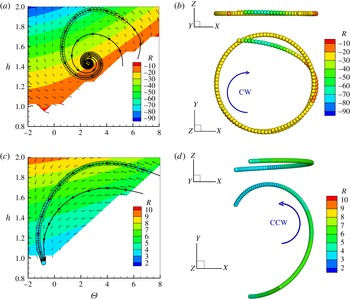
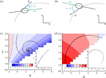
. Figure 3(a) shows the phase plane for a microswimmer close to a solid no-slip surface. Three reduced trajectories, I, II and III are traced. The trajectory III hits the wall while trajectories I and II, although starting from different initial configurations, both converge to the same attractor. The attractor is an asymptotically stable equilibrium point (Cencini, Cecconi & Vulpiani Reference Cencini, Cecconi and Vulpiani2009), (
 $\hat{{\it\Omega}}_{2}$
and
 $\hat{U} _{Z}$
are zero), i.e. nearby trajectories converge to the equilibrium point.
(a) Phase plane
 $\hat{{\it\Theta}}{-}{\hat{h}}$
for a microswimmer close to a rigid no-slip wall. The curvature radius of the trajectory, (3.3), is provided by the colour map. Due to the presence of the wall the blanked regions are forbidden to the swimmer. Three typical trajectories I, II and III are shown by the solid black lines. Trajectories I and II converge to the stable point. The corresponding trajectory in physical space is shown in (b) where the curvature radius in the
 $XY$
-plane is colour coded. Results for the free-slip interface are shown in (c,d). All trajectories eventually intersect the planar interface and no stable orbit exists. Note the opposite sign of the curvature radius in comparison with the no-slip case.

The
 ${\it\phi}$
-averaged trajectory in 3-D space corresponding to I is obtained by integrating the
 ${\it\phi}$
-averaged version of the kinematic equations (2.1), (2.3) and is reported in figure 3(b). Apparently, after a transient, the swimmer stabilizes on a circular clockwise (CW) orbit which corresponds to the stable point in the reduced space
 $(\hat{{\it\Theta}},{\hat{h}})$
. Following Shum et al. (Reference Shum, Gaffney and Smith2010), the curvature radius of the stable orbit is given by
 $$\begin{eqnarray}R=\frac{|\hat{\boldsymbol{U}}(\hat{{\it\bf\Theta}},\hat{\boldsymbol{h}})|}{\hat{{\it\Omega}}_{Z}-\hat{{\it\Omega}}_{X}\tan \hat{{\it\Theta}}},\end{eqnarray}$$
which yields
 $R=-22.1$
. As expected this result matches within numerical accuracy its direct measure
 $R=-21.9$
obtained from the 3-D trajectory, see figure 3(b). Note that (3.3) differs in sign from the original equation given in Shum et al. (Reference Shum, Gaffney and Smith2010) due to a different choice of the body reference frame. It is also worth noting that (3.3) provides the exact curvature radius only for the stable orbit. Nevertheless, it also gives a reasonable approximation in the other conditions here explored, as discussed below. In figure 3(a) the colour map refers to
 $R$
as estimated from (3.3). The colour code in figure 3(b) corresponds to the local curvature radius of the trajectory projection in the
 $xy$
-plane. This information is also reported along the curve I in the phase plane, 3(a), through the colour of the open circles superimposed to the trajectory
 $I$
. From the data it is apparent that the colour differences between the circles and the colour map in the background can hardly be appreciated.
3.2. Swimming in presence of a free-slip interface
The phase plane analysis has been performed for a microswimmer moving close to a free-slip interface, as illustrated in figure 3(c,d). The first significant result is the sign of the curvature radius, now positive, i.e. the swimmer exhibits a counter-clockwise (CCW) motion in contrast to what is observed for the no-slip wall, compare (b) and (d) in figure 3. The curvature radius is smaller with respect to the no-slip case at corresponding
 $(\hat{{\it\Theta}},{\hat{h}})$
. The curvature radius measured in our simulation favourably compares with experimental observation of Di Leonardo et al. (Reference Di Leonardo, Dell Arciprete, Angelani and Iebba2011) where a CCW motion with a curvature radius of
 $\simeq 10~{\rm\mu}\text{m}$
is described. Indeed, assuming
 $\bar{a}=1~{\rm\mu}\text{m}$
, appropriate for an E. coli, the typical radius of curvature found from the present numerics,
 $R\simeq 7$
, gives
 $R^{\prime }=R\bar{a}\simeq 7~{\rm\mu}\text{m}$
.
The second significant result is that no stable trajectory exists when the swimmer moves close to a free surface. In fact, a swimmer similar to an E. coli moving almost parallel to the free surface (low
 $\hat{{\it\Theta}}$
) is always attracted to it. This result confirms the indication of the 2-D model proposed by Crowdy et al. (Reference Crowdy, Lee, Samson, Lauga and Hosoi2011) for undeformable interfaces. This conclusion also partially agrees with the results illustrated by Lopez & Lauga (Reference Lopez and Lauga2014), where the authors, using on a multipole expansion technique, highlighted that the average surface-normal velocity
 $\hat{U} _{z}$
of the swimmer is always negative for
 $\hat{{\it\Theta}}=0$
. Our work adds that the surface is no longer able to attract the swimmer if it swims above a certain height
 $h$
, even with zero tilt angle.
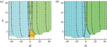
A wider view of the phase plane is displayed for the microswimmer near the no-slip (a) and the free-slip (b) surface. The range exploited in figure 3 corresponds to the small dashed yellow box. Three regions of the phase plane are identified by colours: a trajectory belonging to the light blue region ends colliding with wall, one in the green region escapes and trajectories in the orange region are attracted to the stable orbit. Note that attraction basin is absent in the free-slip case (b). Unstable equilibrium points are marked by the red circles.

In figure 4 we extend our analysis to a wider range of initial conditions, for both no-slip and free-slip surfaces. In both cases, at high positive
 $\hat{{\it\Theta}}$
the microswimmer escapes from the surface while, at high negative
 $\hat{{\it\Theta}}$
, it eventually hits the boundary. On the no-slip wall three cases are possible depending on the initial conditions, namely the swimmer achieves a stable orbit, it escapes from the wall or it collides with the wall. In contrast, for a free-slip surface only two possibilities exist, namely, escaping from the surface or being attracted towards the interface. The maps also highlight the presence of a further equilibrium point
 $(\hat{{\it\Theta}}_{u},{\hat{h}}_{u})$
where the time derivatives of both
 ${\hat{h}}$
and
 $\hat{{\it\Theta}}$
vanish. However, as shown by the behaviour of the streamlines in the neighbourhood of
 $(\hat{{\it\Theta}}_{u},{\hat{h}}_{u})$
, this point is unstable for both no-slip and free-slip cases, i.e. nearby trajectories escape from the equilibrium point.
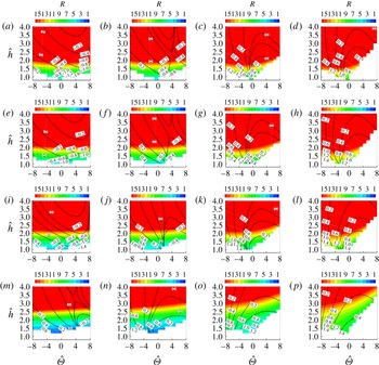
In order to extend the analysis, the dynamics of swimmers with different geometrical characteristics was also examined, focusing in particular on the shape of the head and the tail (axial) length. Figure 5 shows the phase plane
 $\hat{{\it\Theta}}{-}{\hat{h}}$
when the tail length
 $L\in (3,5,10,15)$
and head aspect ratio
 $AR=a_{1}/a_{2}\in (1,3,4,5)$
. When changing the aspect ratio, the swimmer does not substantially modify its behaviour. In particular, the orientation as described by the pitch angle
 $\hat{{\it\Theta}}$
does not qualitatively change and the regions of phase space where the swimmer is attracted to the free surface or where it escapes from it remain very similar. The general trend is an increase of the curvature of the trajectory for given
 $(\hat{{\it\Theta}},\,{\hat{h}})$
as
 $AR$
increases. On the other hand, when changing the relative tail-to-head length, the swimmer hits the wall with different pitch angles
 $\hat{{\it\Theta}}$
. Decreasing the tail length, the region of phase plane where the swimmer escapes becomes larger while the region where it is attracted to the free surface shrinks. The curvature of the trajectory, for given
 $(\hat{{\it\Theta}},\,{\hat{h}})$
, is found to increase with the tail length.
Phase plane
 $\hat{{\it\Theta}}{-}{\hat{h}}$
for a microswimmer close to a free-slip interface for different geometries, namely head aspect ratio
 $AR=a_{1}/a_{2}\in (1,3,4,5)$
(rows, from bottom to top) and tail length
 $L\in (3,5,10,15)$
(columns, from left to right). The colour map corresponds to the curvature radius along trajectories (e.g. solid black lines).

3.3. Drift along the trajectory
Typically the longitudinal axis of the microswimmer is misaligned with the local velocity evaluated at the junction point. This behaviour was experimentally observed for E. coli moving close to a liquid–air interface by Di Leonardo et al. (Reference Di Leonardo, Dell Arciprete, Angelani and Iebba2011). In order to compare with experiments we define the drift angle
 ${\it\alpha}$
as the angle between the
 $X,Y$
projections of the body frame unit vector
 $\boldsymbol{e}_{1}$
and the swimmer velocity
 $\boldsymbol{U}$
. The sign of
 ${\it\alpha}$
is taken to be positive when the swimmer points outward with respect to the trajectory, see figure 6(a).
In figure 6(b,c), the
 ${\it\phi}$
-averaged drift angle is reported for both no-slip and free-slip cases. In the free-slip case the head points outside the trajectory and
 $\hat{{\it\alpha}}$
increases as the swimmer approaches the wall. The spanned range of values,
 $\hat{{\it\alpha}}\in (10^{\circ },30^{\circ })$
, are in good agreement with the experimental observation (Di Leonardo et al.
Reference Di Leonardo, Dell Arciprete, Angelani and Iebba2011). In contrast, in the no-slip case,
 $\hat{{\it\alpha}}$
is slightly negative,
 $\hat{{\it\alpha}}\simeq -2^{\circ }$
, meaning that the swimmer is almost aligned with the trajectory of the reference point
 $\boldsymbol{x}_{J}$
.
(a,b) Sketch illustrating the drift angle
 ${\it\alpha}$
. (c,d) The
 ${\it\phi}$
-averaged drift angle
 $\hat{{\it\alpha}}$
in the phase plane (colour code), for the no-slip and free-slip interface, respectively. Each inset shows a representative trajectory with superimposed the longitudinal unit vector
 $\boldsymbol{e}_{1}$
(the colour coding corresponds to the local value of
 $\hat{{\it\alpha}}$
).

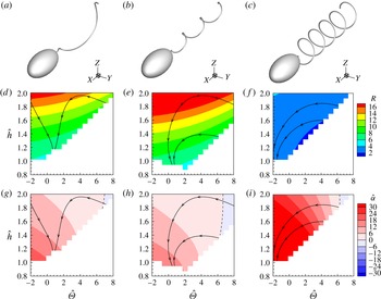
Here, to complete the discussion, the effect of modifying the tail geometry is briefly addressed. Indeed, among the large number of different parameters defining the flagellated geometry, probably the most uncertain ones concern the tail, specifically the amplitude of the helix,
 $A$
, and number of turns,
 $N_{{\it\lambda}}$
. Figure 7 reports the radius of curvature
 $R$
and the drift angle
 $\hat{{\it\alpha}}$
for three different tails. The comparison shows that the results discussed so far are generic.
Different tail geometries. This figure shows the radius of curvature
 $R$
and the drift angle
 $\hat{{\it\alpha}}$
when modifying the tail amplitude
 $A$
or the number of turns
 $N_{{\it\lambda}}$
. Three cases are reported:
 $A=0.8$
and
 $N_{{\it\lambda}}=1$
(a,d,g),
 $A=0.4$
and
 $N_{{\it\lambda}}=3$
(b,e,h),
 $A=0.8$
and
 $N_{{\it\lambda}}=5$
(c,f,i). The hydrodynamic behaviour is qualitatively the same as observed for the reference configuration in figures 3 and 6 with few changes in the variables values.

4. Conclusions
The motion of a flagellated microswimmer close to a boundary, either a solid wall or a free surface, is relevant to several applications spanning from micro-robots to biology and medicine, as concerning in particular biofilm formation. Its dynamics can in principle be affected by several physical phenomena occurring at the microscale and, for biological applications, by the behaviour of the micro-organism. The chemical and physical nature of the interface may play a role in the interaction between the swimmer and the surface, e.g. surface charges and chemicals adsorbed at the interface may have a significant influence. Concerning the specific case of E. coli, taken as representative of most flagellated, recent experimental studies reported a characteristic motion of the swimmer in the two extreme cases of a solid wall and a free surface. In the first case, the experimental observation consistently show that the microswimmer typically moves in circulatory orbits oriented in clockwise direction (CW) (Lauga et al. Reference Lauga, DiLuzio, Whitesides and Stone2006). In contrast, there is evidence that the orientation of the trajectory is reversed (counter clockwise, CCW) when swimming occurs near a free surface Di Leonardo et al. (Reference Di Leonardo, Dell Arciprete, Angelani and Iebba2011). However, the effect of the free surface is less neatly defined and, sometimes, CW motion is reported, probably due to the presence of contaminants adsorbed at the interface (Lemelle et al. Reference Lemelle, Palierne, Chatre and Place2010). Theoretical models proposed to explain this behaviour typically exploit several forms of approximations, e.g. multipole expansion, that may become partially inaccurate when the microswimmer gets very close to the interface.
The present paper provides a complete description of the motion, considering a reasonably realistic geometry of the flagellated in the presence of a free-surface modelled as a rigid, free-slip plane. The resulting model removes any concurrent effect, retaining a full hydrodynamics description. The results for the free-slip boundary were compared with those already analysed in Shum et al. (Reference Shum, Gaffney and Smith2010) for the no-slip case. The data clearly indicate that the motion close to a liquid–air interface is CCW, in agreement with the experimental data (Di Leonardo et al. Reference Di Leonardo, Dell Arciprete, Angelani and Iebba2011) and with the theoretical results obtained by using multipole expansions (Lopez & Lauga Reference Lopez and Lauga2014) and resistive force theory (Di Leonardo et al. Reference Di Leonardo, Dell Arciprete, Angelani and Iebba2011).
Other available experimental information, namely the orientation of the bacteria with respect to its trajectory (Di Leonardo et al. Reference Di Leonardo, Dell Arciprete, Angelani and Iebba2011), are satisfactorily reproduced by the present simulations, confirming that the head of the swimmer points outward. In contrast, the bacteria is roughly aligned with its trajectory close to a no-slip wall. In principle, this observable can be used together with the rotation direction to interpret experimental results on the interaction of a microswimmer with an interface. A characteristic aspect of the motion near a solid surface is the occurrence of stable orbits (Giacché et al. Reference Giacché, Ishikawa and Yamaguchi2010; Shum et al. Reference Shum, Gaffney and Smith2010). On the contrary, no stable orbit has been presently found on a free-slip interface.
In conclusion, the boundary conditions are confirmed to deeply influence the hydrodynamical behaviour of the swimmer. This consideration paves the way to suitably textured surfaces which, properly engineered to stably support a super-hydrophobic state, can be exploited to passively control the microswimmer motion. Indeed the ability of superhydrophobic surfaces to alter the flow has been recently used for passive particle separation (Asmolov et al. Reference Asmolov, Dubov, Nizkaya, Kuehne and Vinogradova2015). In this respect fully-resolved hydrodynamic simulations able to model complex physical surfaces, such as the BEM adopted here, could provide the required fundamental knowledge to extend passive control strategies to active suspensions.
Acknowledgement
The authors acknowledge the CINECA Iscra C Award (IscrC-BSM-LAI) for the availability of HPC resources and the ERC grant no. (339446) BIC: Bubbles from Inception to Collapse.
Appendix A. Green functions for a flat free-slip interface
The Green’s function for a solid adherent wall is known since the work of Blake (Reference Blake1971). The corresponding fundamental solution for a free-slip interface does not seem to be mentioned in the current literature. As shown here, it can be obtained by means of the method of images where the generic localized force is reflected with respect to the plane in such a way to satisfy the impermeability and the zero tangential stress condition. For convenience the index notation is adopted here with
 $\boldsymbol{x}=(x_{1},x_{2},x_{3})$
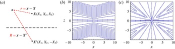
the coordinates of a point in space. The image system is reported in figure 8(a) where the point force
 $\boldsymbol{b}=(b_{1},b_{2},b_{3})$
placed at
 $\boldsymbol{X}=(X_{1},X_{2},X_{3})$
is reflected in
 $\boldsymbol{X}^{\prime }=(X_{1},X_{2},-X_{3})$
as
 $\boldsymbol{b}^{\prime }=(b_{1},b_{2},-b_{3})$
. The relative positions
 $$\begin{eqnarray}\displaystyle & \displaystyle \boldsymbol{r}=\boldsymbol{x}-\boldsymbol{X}=(x_{1}-X_{1},x_{2}-X_{2},x_{3}-X_{3}), & \displaystyle\end{eqnarray}$$
 $$\begin{eqnarray}\displaystyle & \displaystyle \boldsymbol{r}^{\prime }=\boldsymbol{x}-\boldsymbol{X}^{\prime }=(x_{1}-X_{1},x_{2}-X_{2},x_{3}+X_{3}), & \displaystyle\end{eqnarray}$$
 $\boldsymbol{x}$
in the fluid domain with the two singularities in
 $\boldsymbol{X}$
and
 $\boldsymbol{X}^{\prime }$
, respectively. Taking into account the well-known expression for the free space Green function (Happel & Brenner Reference Happel and Brenner1983)
 $$\begin{eqnarray}\unicode[STIX]{x1D60E}_{ij}^{free}=\left(\frac{{\it\delta}_{ij}}{r}+\frac{r_{i}r_{j}}{r^{3}}\right),\end{eqnarray}$$
the superposition of the two singularities yields
 $$\begin{eqnarray}\displaystyle & \displaystyle \unicode[STIX]{x1D60E}_{i1}^{FS}=\left(\frac{{\it\delta}_{i1}}{r}+\frac{r_{i}r_{1}}{r^{3}}\right)+\left(\frac{{\it\delta}_{i1}}{r^{\prime }}+\frac{r_{i}^{\prime }r_{1}^{\prime }}{r^{\prime 3}}\right), & \displaystyle\end{eqnarray}$$
 $$\begin{eqnarray}\displaystyle & \displaystyle \unicode[STIX]{x1D60E}_{i2}^{FS}=\left(\frac{{\it\delta}_{i2}}{r}+\frac{r_{i}r_{2}}{r^{3}}\right)+\left(\frac{{\it\delta}_{i2}}{r^{\prime }}+\frac{r_{i}^{\prime }r_{2}^{\prime }}{r^{\prime 3}}\right), & \displaystyle\end{eqnarray}$$
 $$\begin{eqnarray}\displaystyle & \displaystyle \unicode[STIX]{x1D60E}_{i3}^{FS}=\left(\frac{{\it\delta}_{i3}}{r}+\frac{r_{i}r_{3}}{r^{3}}\right)-\left(\frac{{\it\delta}_{i3}}{r^{\prime }}+\frac{r_{i}^{\prime }r_{3}^{\prime }}{r^{\prime 3}}\right). & \displaystyle\end{eqnarray}$$
 $i$
th velocity component at
 $\boldsymbol{x}$
is expressed in terms of the force intensity
 $\boldsymbol{b}$
at
 $\boldsymbol{X}$
as
 $$\begin{eqnarray}u_{i}(\boldsymbol{x})=\frac{1}{8{\rm\pi}{\it\mu}}\unicode[STIX]{x1D60E}_{ij}^{FS}(\boldsymbol{x},\boldsymbol{X})b_{j}.\end{eqnarray}$$
It can be immediately checked that the ensuing velocity field satisfies impermeability and free-slip conditions at
 $x_{3}=0$
. Indeed, as concerning the wall-normal velocity, impermeability straighforwardly follows from (A 7). Let us consider now the zero tangential stress condition. From the stress tensor associated with (A 7)
 $$\begin{eqnarray}\displaystyle & \displaystyle \unicode[STIX]{x1D61B}_{ik1}^{FS}=-6\frac{r_{i}r_{1}r_{k}}{r^{5}}-6\frac{r_{i}^{\prime }r_{1}^{\prime }r_{k}^{\prime }}{r^{\prime 5}}, & \displaystyle\end{eqnarray}$$
 $$\begin{eqnarray}\displaystyle & \displaystyle \unicode[STIX]{x1D61B}_{ik2}^{FS}=-6\frac{r_{i}r_{2}r_{k}}{r^{5}}-6\frac{r_{i}^{\prime }r_{2}^{\prime }r_{k}^{\prime }}{r^{\prime }}, & \displaystyle\end{eqnarray}$$
 $$\begin{eqnarray}\displaystyle & \displaystyle \unicode[STIX]{x1D61B}_{ik3}^{FS}=-6\frac{r_{i}r_{3}r_{k}}{r^{5}}+6\frac{r_{i}^{\prime }r_{3}^{\prime }r_{k}^{\prime }}{r^{\prime }}, & \displaystyle\end{eqnarray}$$
 $x_{3}=0$
vanishes identically, i.e.
 $\unicode[STIX]{x1D61B}_{i3j}^{FS}b_{j}=0$
for
 $i=1,2$
. An illustration is provided in figure 8(b,c) where the streamlines associated with the free-slip Green function due to a point force respectively parallel
 $\boldsymbol{b}=(1,0,0)$
and normal
 $\boldsymbol{b}=(0,0,1)$
to the wall placed at
 $X=(0,0,1)$
are reported.
(a) The image system employed to obtain the Green function for a planar free-slip interface. (b,c) The streamlines in the
 $x_{2}=0$
plane, due to a point force
 $\boldsymbol{b}=(1,0,0)$
in
 $\boldsymbol{X}=(0,0,1)$
and a point force
 $\boldsymbol{b}=(0,0,1)$
in
 $\boldsymbol{X}=(0,0,1)$
, respectively. In both cases the velocity at the interface is purely parallel to the
 $x_{3}=0$
plane, as required by the impermeability. The symmetry of the fields with respect to
 $x_{3}=0$
implies the vanishing of the tangential shear stress at the interface.