1 Introduction
Microturbulence driven by small Larmor-scale instabilities is, in most cases, the dominant cause of heat and particle loss from the core of magnetic confinement fusion devices and therefore presents a major challenge in achieving burning plasma conditions (Horton Reference Horton1999). The role of passing electron dynamics in turbulent transport driven by ion-scale microinstabilities, in particular ion temperature gradient (ITG) and trapped electron mode (TEM) instabilities, has been given relatively little attention. In first approximation, these particles, which are highly mobile along the confining magnetic field, are assumed to respond adiabatically to the low-frequency ion-scale modes. However, in a tokamak geometry, the phase velocity parallel to the magnetic field of a perturbation with fixed mode numbers  $m$ and
 $n$ in the poloidal and toroidal directions, respectively, becomes infinite at the radial position
 $r_{m,n}$ of the corresponding mode rational surface (MRS), where the magnetic safety factor profile
 $q_s(r)$ is such that
 $q_s(r_{m,n}) = m/n$. Consequently, at these positions, the condition for passing electrons to respond adiabatically is violated and their non-adiabatic response becomes important. One notes that, given the toroidal axisymmetry of a tokamak, each linear microturbulence eigenmode has a fixed toroidal mode number
 $n$, but is, in general, a superposition of many poloidal Fourier modes
 $m$, so that associated MRSs are the positions
 $r_{m,n}$ for the different values of
 $m$.
In fact, as a result of the non-adiabatic passing electron dynamics, linear ITG and TEM eigenmodes can become significantly extended along the magnetic field lines (Hallatschek & Dorland Reference Hallatschek and Dorland2005), producing fine radial structures at corresponding MRSs (Falchetto, Vaclavik & Villard Reference Falchetto, Vaclavik and Villard2003; Chowdhury et al. Reference Chowdhury, Ganesh, Angelino, Vaclavik, Villard and Brunner2008). These fine structures on the eigenmodes persist in corresponding turbulence simulations, and via non-linear couplings lead to stationary corrugations on the radial profiles of density, temperature and, in particular,  $E\times B$ zonal shear flows, aligned with low-order MRSs, which effectively appear as fine-scale transport barriers (Waltz et al. Reference Waltz, Austin, Burrell and Candy2006; Dominski et al. Reference Dominski, Brunner, Görler, Jenko, Told and Villard2015, Reference Dominski, McMillan, Brunner, Merlo, Tran and Villard2017). Given that shearing and decorrelation of turbulent eddies by zonal flows is a primary mechanism by which turbulence saturates (Biglari, Diamond & Terry Reference Biglari, Diamond and Terry1990; Waltz, Kerbel & Milovich Reference Waltz, Kerbel and Milovich1994; Lin et al. Reference Lin, Hahm, Lee, Tang and White1998; Rosenbluth & Hinton Reference Rosenbluth and Hinton1998), it is clearly of interest to understand the generation of these fine-scale zonal flow structures in detail.
The generation of the fine zonal flow structures at low-order MRSs, via a process called self-interaction, has in fact already been discussed to some length in the work by Weikl et al. (Reference Weikl, Peeters, Rath, Seiferling, Buchholz, Grosshauser and Strintzi2018). The general motivation for the work presented in this paper has been to further investigate the properties of zonal flow drive from this self-interaction mechanism. This process essentially involves each individual microturbulence eigenmode interacting non-linearly with itself to produce a Reynolds stress contribution to the zonal flow drive, which turns out to be located around its corresponding MRSs. Key to this self-interaction is the fact that an eigenmode that is significantly extended along the magnetic field line ‘bites its tail’ after one poloidal turn. For each eigenmode, self-interaction will therefore be particularly significant at its MRSs, given that the radially fine structures located at these positions, resulting from the non-adiabatic passing electron response, are elongated along the magnetic field lines. At low-order MRSs (in practice, implying mainly integer and half-integer  $q_s$ surfaces), these self-interaction contributions to Reynolds stress from the different eigenmodes radially align and add up constructively to drive the stationary
 $E\times B$ zonal shear flows. Clear illustrations of these fine stationary zonal flow structures can be seen for example in figure 2 of Waltz et al. (Reference Waltz, Austin, Burrell and Candy2006), figure 12 of Dominski et al. (Reference Dominski, McMillan, Brunner, Merlo, Tran and Villard2017), figure 3 of Weikl et al. (Reference Weikl, Peeters, Rath, Seiferling, Buchholz, Grosshauser and Strintzi2018) and figure 4 of the present paper.
It is important to point out that in the core of a tokamak, low-order MRSs are, in fact, few and far apart, whereas the radial domains between them occupy the majority of the plasma volume. Therefore, at least as important as understanding how self-interaction generates the above-mentioned stationary structures at lowest-order MRSs (LRMSs), clearly visible on any flux surface-averaged field, is to address how the same self-interaction mechanism might affect zonal flow drive and, therefore, turbulent transport in the radial regions between low-order MRSs. Addressing this question is the main focus of this paper.
Although LMRSs are common to all eigenmodes, between them, the MRSs related to the various microturbulence modes tend to be radially misaligned. Hence, in these radial regions, the self-interaction contributions to Reynolds stress from these modes tend to cancel each other out when averaged over time, thus resulting in a nearly zero stationary component of the zonal flows. However, given that in the turbulent phase amplitudes of the various microinstability eigenmodes vary in time and, furthermore, are decorrelated with each other, this cancellation is not ensured at each time instant, but only on average over time. As a result, self-interaction drives a non-zero fluctuating zonal flow component between low-order MRSs.
An important observation resulting from our study is that in simulations accounting for non-adiabatic passing electron dynamics, self-interaction contributions to Reynolds stress from the various microturbulence modes can indeed be significant in the radial regions between LMRSs and, in fact, act as random decorrelated kicks that can in some cases actually disrupt what is usually considered the main drive mechanism of zonal flows: modulational instability (Hasegawa & Mima Reference Hasegawa and Mima1978; Hasegawa, Maclennan & Kodama Reference Hasegawa, Maclennan and Kodama1979; Chen, Lin & White Reference Chen, Lin and White2000). The modulational instability mechanism involves the resonant decays of microinstability modes into zonal modes via secondary microinstability daughter modes. Unlike self-interaction, it is a coherent process, leading to a correlated contribution from the various microinstability modes to the Reynolds stress drive of zonal modes.
To quantify the relative importance of the two alternative, possibly competing mechanisms driving zonal flows, i.e. self-interaction and modulational instability, we have studied the statistical properties of the Reynolds stress contributions from the various microturbulence modes. Given the different nature of the two driving processes, one can identify high correlation levels between the mode contributions to conditions where modulational instability drive dominates, whereas lower correlation levels are characteristic of a significant effect from self-interaction. Central to this statistical analysis has been a series of gyrokinetic simulations obtained for identical driving conditions but varying the number of significant toroidal modes participating in the turbulence. Varying the number of toroidal modes changes, in particular, the number of associated random kicks from self-interaction to the zonal flow drive at each radial position.
Varying the number of significant toroidal modes is, in fact, related to varying the system size, typically measured by  $\rho ^{\star } = \rho _i/a$, i.e. the ratio of the thermal ion Larmor radius
 $\rho _i$ to the minor radius
 $a$ of the tokamak. Indeed, invoking the fact that the unstable modes driving ion-scale microturbulence are such that
 $k_\perp \rho _i \lesssim 1$, where
 $k_\perp$ is the wave vector component perpendicular to the magnetic field, and furthermore noting that for a given eigenmode with toroidal mode number
 $n$, an estimate for
 $k_\perp$ is given by the poloidal wave vector component, which in turn can be evaluated as
 $k_\chi \simeq m/r_0\simeq nq_s(r_0)/r_0$ (
 $r_0$ is the average radial position of the eigenmode and
 $m$ its characteristic poloidal mode number estimated as
 $m\simeq nq_s(r_0)$, given that fluctuations are nearly field-aligned), one obtains that
 $k_\perp \rho _i \simeq nq_s(r_0)\rho _i/r_0 = (q_s a/r_0) n\rho ^{\star } \sim n\rho ^{\star }$, so that the number
 $N_\varphi$ of toroidal modes contributing to the turbulence scales as
 $N_\varphi \sim 1/\rho ^{\star }$.
In view of what has just been stated, it may at first sight appear surprising that the study presented in this paper is, in fact, based on simulations carried out in the framework of the flux-tube model (Beer, Cowley & Hammett Reference Beer, Cowley and Hammett1995), whose underlying assumption is the scale separation between the characteristic length of microturbulence ( $\sim$ Larmor radius
 $\rho$) and the characteristic length of equilibrium (
 $\sim$ minor radius
 $a$), hence a priori achieved by taking the strict limit
 $\rho ^{\star }\to 0$ of the gyrokinetic equations. In this limit, the radial dependence of all equilibrium profiles and their gradients appearing in the gyrokinetic equations are constant over the flux-tube volume. There is, however, one exception to this in the standard flux tube model (Scott Reference Scott1998): a linearised radial dependence of the safety factor profile
 $q_s(r)$ (
 $\sim$ constant magnetic shear approximation) is kept in the twist and shift boundary condition applied after usually following the magnetic field line a single turn in the poloidal direction. Through this parallel boundary condition, an eigenmode ‘bites its tail’ and, in particular, correctly accounts for the possible resonances that may develop at its associated MRSs. The fact that the eigenmodes correctly ‘feel’ their associated MRSs is obviously key to the development of the fine radial structures and related non-linear self-interaction which is the focus of our study. In addition, close agreement between flux-tube (Dominski et al. Reference Dominski, Brunner, Görler, Jenko, Told and Villard2015) and global (Dominski et al. Reference Dominski, McMillan, Brunner, Merlo, Tran and Villard2017) gyrokinetic simulations regarding the characteristics of the fine stationary zonal flow structures at LMRSs clearly confirm that the dynamics of the self-interaction mechanism can indeed be correctly accounted for using such a local model.
Let us already briefly provide here some further insight into how the toroidal spectral density is varied in a flux-tube code (all details will be given in § 2). The flux-tube version of the GENE code (Jenko et al. Reference Jenko, Dorland, Kotschenreuther and Rogers2000; Merz Reference Merz2008) that we have applied for the present study, considers the field-aligned coordinate system defined (in (2.1)–(2.3)) by the variables  $(x, y, z)$, which are the radial, binormal and parallel coordinates, respectively. Note that the binormal coordinate
 $y$ is the only one of the three coordinates
 $(x, y, z)$ that actually depends on the toroidal angle
 $\varphi$. The length
 $L_y$ of the flux tube in this direction can, thus, be associated to its angular extent
 ${\rm \Delta} \varphi$ along
 $\varphi$:
 $L_y = C_y{\rm \Delta} \varphi$, where the constant
 $C_y = r_0/q_0$ ensures that
 $y$ has units of length,
 $r_0$ being the radial position at which the flux tube is positioned and
 $q_0 = q_s(r_0)$. In addition, as a linear eigenmode has a fixed toroidal mode number
 $n$, it consequently has a fixed Fourier mode number
 $k_y$ with respect to
 $y$ when represented in field-aligned coordinates, given by
 $k_y = n/C_y = nq_0/r_0$, i.e.
 $k_y$ is actually equivalent to the previously mentioned poloidal mode number estimate
 $k_\chi$. The significant
 $k_y$ modes contributing to ion-scale turbulence are, therefore, such that
 $k_y\rho _i \lesssim 1$, and given that the minimum mode number for a flux-tube box with length
 $L_y$ is given by
 $k_{y,\min }=2{\rm \pi} /L_y$, the number of toroidal modes contributing to the turbulence is estimated as
 $N_\varphi \simeq 1/k_{y,\min }\rho _i= (1/2{\rm \pi} )L_y/\rho _i$. Hence, when studying microturbulence using flux-tube simulations, carrying out a scan in
 $k_{y,\min }\rho _i$ (or, equivalently,
 $L_y/\rho _i$) corresponds to varying the toroidal spectral density.
In view of these results, it is therefore possible to realistically study the importance of the self-interaction mechanism via a flux-tube simulation for a given size tokamak, characterised by a finite  $\rho ^{\star }$ value, by considering the appropriate toroidal spectral density, i.e. by setting
 $k_{y,\min }\rho _i = \rho _i/C_y=(q_0a/r_0)\rho ^{\star }$ corresponding to the toroidal mode number
 $n=1$ (one naturally recovers here that the number of modes contributing to turbulence scales as
 $N_\varphi \simeq 1/k_{y,\min }\rho _i\sim 1/\rho ^{\star }$). This is clearly equivalent to setting
 $L_y= 2{\rm \pi} C_y$, i.e.
 ${\rm \Delta} \varphi =2{\rm \pi}$, which along with parallel box length
 $L_z=2{\rm \pi}$ implies having the flux tube cover the full magnetic surface once. Therefore, considering a finite
 $k_{y,\min }\rho _i$ value in a flux-tube simulation effectively corresponds to accounting for a finite
 $\rho ^{\star }$ effect. All other finite
 $\rho ^{\star }$ effects such as profile shearing (Waltz, Dewar & Garbet Reference Waltz, Dewar and Garbet1998; Waltz, Candy & Rosenbluth Reference Waltz, Candy and Rosenbluth2002), or finite radial extent of the unstable region (McMillan et al. Reference McMillan, Lapillonne, Brunner, Villard, Jolliet, Bottino, Goerler and Jenko2010), are however obviously absent in a flux tube.
Given that  $k_{y\min }\rho _i \sim \rho ^{\star }$, the true flux-tube model would require considering the limit of
 $k_{y\min }\rho _i \to 0$. In numerical simulations, however, for obvious practical reasons,
 $k_{y\min }\rho _i\sim \rho _i/L_y$ is always finite, so that if turbulence actually converges for
 $k_{y\min }\rho _i \to 0$, this limit can at best be approximately approached in the limit of large box length
 $L_y/\rho _i$, which may become numerically prohibitive. Thus, carrying out the above-mentioned
 $k_{y,\min }\rho _i$ scan also enables us to investigate whether/how the flux-tube simulation results converge as
 $k_{y,\min }\rho _i\rightarrow 0$, a problem that was already addressed in our sister paper (Ball, Brunner & C. J. Reference Ball, Brunner and C. J.2020). It is remarkable that, to the best of the authors’ knowledge, the convergence of flux-tube gyrokinetic turbulence simulations with respect to
 $k_{y\min }\rho _i$ seems not to have been given more attention in the literature, at least not considering fully kinetic electron dynamics. Our simulations of ITG-driven turbulence indeed illustrate that for practical values of
 $k_{y,\min }\rho _i$, typically chosen in the range
 $10^{-2}\text {--}10^{-1}$, convergence of turbulent fluxes is in many cases not yet reached. In particular, in the case of strong background temperature gradients, i.e. away from marginal stability, the gyro-Bohm normalised ion heat flux
 $Q_i$ keeps on increasing with a nearly algebraic scaling
 $Q_i \sim (k_{y,\min }\rho _i)^{\alpha }$,
 $\alpha > 0$, when decreasing
 $k_{y,\min }\rho _i$, thus showing no apparent sign of convergence within this range of values. In the particular strong gradient case considered, corresponding to parameters near to the cyclone base case (CBC) (Dimits et al. Reference Dimits, Bateman, Beer, Cohen, Dorland, Hammett, Kim, Kinsey, Kotschenreuther and Kritz2000), one has
 $\alpha \simeq 0.45$ (see figure 7 in the present paper), so that
 $Q_i$ increases by nearly a factor of
 $3$ over the range
 $k_{y,\min }\rho _i = 10^{-2}\text {--}10^{-1}$. In agreement with related work by one of our co-authors (Ball et al. Reference Ball, Brunner and C. J.2020), for sufficiently small values of
 $k_{y,\min }\rho _i$, the algebraic scaling is ultimately broken and convergence of the fluxes is finally approached within
 ${\sim }5\,\%$ for
 $k_{y,\min }\rho _i \simeq 5\times 10^{-3}$ (see figure 18 in the present paper). However, this corresponds to a value of
 $k_{y,\min }\rho _i$, one order of magnitude smaller than usually considered. For gradients closer to marginal stability, this dependence of
 $Q_i$ on
 $k_{y,\min }\rho _i$ appears to be weakened and convergence approached already for somewhat larger, numerically more affordable values. This can be seen as good news, as gradients near marginal stability may be considered as the physically most relevant cases. It nonetheless appears essential that one keeps in mind this potentially significant dependence of the fluxes on
 $k_{y,\min }\rho _i$ in the range of typically considered values, which seems to have very often been overlooked or at least not been given sufficient attention in past studies.
In conjunction with the observed increase in fluxes with system size over the considered range of  $k_{y,\min }\rho _i=10^{-2}\text {--}10^{-1}$, a decrease in the shearing rate associated to fluctuating zonal flows is also observed (see figure 6c). Via a simple ‘back-of-the-envelope’ estimate, this decrease in the shearing rate associated with fluctuating zonal flows is shown to result from the fact that the self-interaction drive of zonal flows from the various microturbulence modes are decorrelated with each other.
The remainder of this paper is organised as follows.
Important aspects of the flux-tube version of the grid-based gyrokinetic code GENE (Jenko et al. Reference Jenko, Dorland, Kotschenreuther and Rogers2000; Merz Reference Merz2008; Görler et al. Reference Görler, Lapillonne, Brunner, Dannert, Jenko, Merz and Told2011), which was used for performing the simulations in this study, are presented in § 2. Details of its field-aligned coordinate system are recalled, in particular how the parallel boundary conditions ensure that linear eigenmodes correctly ‘feel’ associated MRSs.
A brief summary of a set of previous studies (Dominski et al. Reference Dominski, Brunner, Görler, Jenko, Told and Villard2015, Reference Dominski, McMillan, Brunner, Merlo, Tran and Villard2017), addressing the role of non-adiabatic passing electron dynamics and which provided the starting point for the main work presented in this paper, is given in § 3. The same ITG-driven turbulence case as in Dominski et al. (Reference Dominski, Brunner, Görler, Jenko, Told and Villard2015) will, in fact, also be considered as a reference case here. Its parameters are recalled as well as the linear frequency and growth rate spectra. Also pointed out are the fine radial structures that develop on the linear eigenmodes as a result of the non-adiabatic passing electron dynamics. Furthermore summarised is how these fine structures on the eigenmodes act as channels for electron heat and particle transport, and, through non-linear coupling, are observed to lead to corrugations at low-order MRSs of the time-averaged density and temperature profiles as well as  $E\times B$ zonal flow shear layers.
The main results for the present study, consisting of non-linear flux-tube simulations of ITG-driven turbulence, are presented in § 4. Sets of simulations have been obtained by scanning  $k_{y,\min }\rho _i$ over the typical range of values considered in practice, i.e.
 $k_{y,\min }\rho _i = 10^{-2}\text {--}10^{-1}$. These scans were repeated considering ITGs both near and far from marginal stability. Furthermore, to clearly illustrate how the fine radial structures resulting from the non-adiabatic passing electron dynamics lead to particularly strong contributions to zonal flow drive from the self-interaction mechanism, simulations with two different electron models were carried out: either considering fully kinetic electron dynamics or enforcing their fully adiabatic response (fine radial structures being absent with the latter model). First analysis of results are carried out in this same section, showing that especially in the case of fully kinetic electrons and far from marginal stability, heat fluxes
 $Q_i$ have not yet converged over the considered range of typical
 $k_{y,\min }\rho _i$ values. Given its key role in saturating ITG-driven turbulence, the level of zonal flow shearing rate,
 $\omega _{E\times B}$, is carefully diagnosed. It is shown how in all cases this shearing rate decreases with decreasing
 $k_{y,\min }\rho _i$ (see figure 6). Also analysed is the radial correlation length of the turbulence. An important observation is that for sufficiently small
 $k_{y,\min }\rho _i$, the radial extent of turbulent eddies presents a clearly shorter scale length than the distance between LMRSs (figure 8). From this one concludes that, for these lower values of
 $k_{y,\min }\rho _i$, the turbulence is mostly sheared by the zonal flows between LMRSs, where
 $\omega _{E\times B}$ is essentially composed of its fluctuating component, rather then sheared by the stationary component of
 $\omega _{E\times B}$ located at the LMRSs.
Section 5 is dedicated to understanding why fluctuating zonal shear flow level decreases with  $k_{y,\min }\rho _i$. To this end, the different zonal flow driving mechanisms are analysed in detail. After showing in § 5.1 that Reynolds stress can be considered as a proxy for measuring the drive of zonal flows, we review the two basic zonal flow driving mechanisms: modulational instability in § 5.2 and self-interaction in § 5.3. To illustrate these two basic mechanisms, reduced non-linear simulations are presented in § 5.4, where the drive of zonal modes via the decay of an initially single finite-amplitude ITG eigenmode is studied. These simulations are carried out with both adiabatic and kinetic electrons to demonstrate the dominant role of modulational instability in the former case and the significant role of self-interaction in the latter.
Evidence of the self-interaction and the modulational instability mechanisms in fully developed turbulence is then addressed in §§ 5.5 and 5.6, respectively. A comparison between simulations with adiabatic and kinetic electrons is done here as well. It is shown that the self-interaction mechanism is persistent in the turbulence simulations accounting for fully kinetic electrons, whereas it is weak in simulations with adiabatic electrons, consistent with the reduced non-linear simulations. Using statistical methods such as bicoherence and Reynolds stress correlation analysis diagnostics, we show that the self-interaction contributions to Reynolds stress from the various microturbulence modes are decorrelated in time, and essentially act as random kicks on the zonal modes, whereas the contributions from modulational instability, which is a coherent process, are correlated with each other. In the case of adiabatic electron simulations, strong correlation between Reynolds stress contributions from different modes as well as large bicoherence levels are measured, reflecting that self-interaction is indeed weak and zonal flow drive is dominated by the modulational instability. In the case of kinetic electrons, however, self-interaction may disrupt the zonal flow drive from modulational instability and, consequently, correlation between Reynolds stress contributions as well as bicoherence levels are found to be relatively weak (see figures 15 and 16).
Based on the study carried out in § 5, providing evidence of the decorrelated nature of the self-interaction contributions to zonal flow drive from the various microturbulence modes, we carry out a ‘back-of-the-envelope’ derivation, using simple statistical arguments, to predict the scaling observed in simulations with kinetic electrons of the zonal flow shearing rate  $\omega _{E\times B}$ with
 $k_{y,\min }\rho _i$. This derivation is presented in § 6.
The final discussion and conclusions are provided in § 7.
2 The GENE flux-tube model
GENE is an Eulerian electromagnetic gyrokinetic code. The flux-tube version of the code is used in this study. In view of the issues addressed in this paper, we recall some important features of the flux-tube model (scaling assumptions, field-aligned coordinate system and boundary conditions).
GENE uses a non-orthogonal, field-aligned coordinate system  $(x, y, z)$ defined in terms of the magnetic coordinates
 $(\psi , \chi , \varphi )$ as follows (Beer et al. Reference Beer, Cowley and Hammett1995):
 \begin{gather} x = x(\psi){:}\ \text{radial coordinate,} \end{gather}
 \begin{gather}y = C_y[q_s(\psi)\chi-\varphi]{:}\ \text{binormal coordinate,} \end{gather}
 \begin{gather}z = \chi{:} \ \text{parallel coordinate.} \end{gather}
Here  $\psi , \chi$ and
 $\varphi$ represent the poloidal magnetic flux, straight field line poloidal angle and the toroidal angle, respectively. The function
 $x(\psi )$ is a function of
 $\psi$ with units of length and
 $C_y=r_0/q_0$ is a constant, where
 $q_0$ is the safety factor at
 $r_0$ denoting the radial position of the flux tube. The inverse aspect ratio of the flux tube is defined as
 $\epsilon =r_0/R$, where
 $R$ is the major radius of the tokamak.
The flux-tube model assumes a scale separation between the radial correlation length of turbulent eddies ( ${\sim }\rho _i$) and the radial length scale of variation of equilibrium (
 ${\sim }a$), thus corresponding to the limit
 $\rho ^{*}=\rho _i/a \ll 1$. Consistent with this scale separation, the background density and temperature gradients, as well as the magnetic equilibrium quantities, are considered constant across the radial extension
 $L_x$ of the flux tube, and are evaluated at
 $r_0$. An exception is the safety factor appearing in the parallel boundary condition, discussed in detail later in this section. The background density and temperature of a species
 $j$ are, respectively,
 $N_{j,0}=N_{j,0}(r_0)$ and
 $T_{j,0}=T_{j,0}(r_0)$ and their inverse radial gradients lengths are
 $1/L_{Nj}=-\textrm {d}\log N_{j,0}/\textrm {d}r|_{r=r_0}$ and
 $1/L_{Tj}=-\textrm {d}\log T_{j,0}/\textrm {d}r|_{r=r_0}$. The magnetic field amplitude
 $B_0=B_0(z)$, Jacobian
 $\mathcal {J}^{xyz}=\mathcal {J}^{xyz}(z)$ and the metric coefficients
 $g^{\mu \nu }(z)=\boldsymbol {\nabla }\mu \boldsymbol {\cdot }\boldsymbol {\nabla }\nu$ where
 $\mu$ and
 $\nu$ are the flux-tube coordinates
 $(x,y,z)$, depend only on the parallel coordinate.
The flux-tube coordinates  $(x,y,z)$ satisfy the double periodic boundary condition in a tokamak as follows. The
 ${\rm \Delta} \varphi$-periodicity of any physical quantity
 $\mathcal {A}$, in particular fluctuations, along the toroidal direction
 $\varphi$ reads
 \begin{equation} \mathcal{A}(\psi,\chi,\varphi+{\rm \Delta}\varphi)=\mathcal{A}(\psi,\chi,\varphi), \end{equation}
and translates in  $(x, y, z)$ coordinates to an
 $L_y$-periodicity along
 $y$:
 \begin{equation} \mathcal{A}(x,y+L_y,z)=\mathcal{A}(x,y,z), \end{equation}
where  $L_y=C_y{\rm \Delta} \varphi$. If the flux tube covers the full flux surface,
 ${\rm \Delta} \varphi =2{\rm \pi}$, otherwise
 ${\rm \Delta} \varphi$ is only a fraction of
 $2{\rm \pi}$. The
 $2{\rm \pi}$-periodicity in the poloidal direction
 $\chi$ reads
 \begin{equation} \mathcal{A}(\psi,\chi+2{\rm \pi},\varphi)=\mathcal{A}(\psi,\chi,\varphi), \end{equation}
and translates in  $(x, y, z)$ coordinates to a pseudo-periodic condition along
 $z$:
 \begin{equation} \mathcal{A}(x,y+C_yq_s(x)2{\rm \pi}, z+2{\rm \pi})=\mathcal{A}(x,y,z). \end{equation}
This boundary condition is referred to as the parallel boundary condition (Scott Reference Scott1998). Note that in the flux-tube model in general, one can consider a periodicity in  $z$ that is larger than
 $2{\rm \pi}$ as well (Beer et al. Reference Beer, Cowley and Hammett1995; Faber et al. Reference Faber, Pueschel, Terry, Hegna and Roman2018; Ball et al. Reference Ball, Brunner and C. J.2020). However, typically the
 $2{\rm \pi}$-periodicity is considered, as it is in this work.
Furthermore, the radial scale separation  $\rho ^{*}\ll 1$ justifies periodic boundary conditions along
 $x$:
 \begin{equation} \mathcal{A}(x+L_x, y, z)=\mathcal{A}(x,y,z). \end{equation}
Given the periodicity along  $x$ and
 $y$ expressed by (2.8) and (2.5), a Fourier series decomposition is a practical representation of fluctuation fields as it naturally verifies these boundary conditions. Such a Fourier representation reads
 \begin{equation} \mathcal{A}(x, y, z) = \sum_{k_x, k_y} \hat{\mathcal{A}}_{k_x, k_y}(z)\exp[\textrm{i}(k_xx+k_yy)], \end{equation}
with  $k_x$ and
 $k_y$ corresponding, in general, to all harmonics of the minimum wave numbers
 $k_{x, \min } = 2{\rm \pi} /L_x$ and
 $k_{y, \min } = 2{\rm \pi} /L_y$ respectively.
The underlying axisymmetry of a tokamak corresponds to an invariance of the unperturbed system with respect to  $\varphi$ in
 $(\psi , \chi , \varphi )$ coordinates. This translates to an invariance with respect to
 $y$ in
 $(x,y,z)$ coordinates. Consequently, any fluctuating field related to a linear eigenmode of the toroidal system is, thus, composed of a single
 $k_y$ Fourier mode. Note that a given
 $k_y$ wave number is equivalent to a toroidal wave number
 $n$ according to the relation
 \begin{equation} n=-k_yC_y. \end{equation}
It remains to express the pseudo-periodic boundary condition (2.7) in the Fourier representation (2.9). In doing so, one considers the  $x$-dependence of the safety factor profile
 $q_s(x)$. This is essential to ensure that the flux-tube model contains the information on the radial position of MRSs related to a
 $k_y$ mode and thus accounts for the particular dynamics, in particular resonances, that can take place at such surfaces. This is of key importance to the study carried out in this paper. Accounting for the
 $x$-dependence of the safety factor in these boundary conditions is thus an exception in the flux-tube framework, as all other background and magnetic geometry coefficients, as already mentioned, are assumed
 $x$-independent. Only a linearised safety factor profile of the form:
 \begin{equation} q_s(x)=q_0[1+\hat{s}(x-x_0)/r_0], \end{equation}
with  $\hat {s}$ standing for the magnetic shear, is in fact compatible with the Fourier representation along
 $x$. For a given
 $k_y$ Fourier mode, inserting (2.9) and (2.11) into (2.7) leads to
 \begin{equation} \sum_{k_x} \hat{\mathcal{A}}_{k_x, k_y}(z+2{\rm \pi}) \exp[2{\rm \pi} \textrm{i} k_yC_yq_s(x=0)] \exp[\textrm{i} (k_x + 2{\rm \pi} k_y\hat{s})x] = \sum_{k_x} \hat{\mathcal{A}}_{k_x, k_y}(z) \exp(\textrm{i} k_x x). \end{equation}
For convenience and without further loss of generality, one assumes here that the origin of the  $x$ coordinate corresponds to the LMRS, i.e. a MRS related to
 $k_{y, \min }$. This condition reads
 \begin{equation} k_{y, \min}C_yq_s(x=0) = n_{\min} q_s(x=0) = n_{\min} q_0(1-\hat{s}x_0/r_0) \in \mathbb{Z}, \end{equation}
with  $n_{\min }$ the toroidal wave number associated with
 $k_{y, \min }$. Note that this relation provides an equation for the shift in
 $x_0$ and ensures that the phase factor
 $\exp [2{\rm \pi} \textrm {i}k_yC_yq_s(x=0)]=1$ for all
 $k_y$ modes. Based on (2.12), the boundary condition in
 $z$ then finally translates for a given
 $k_y$ Fourier mode to the following coupling between
 $k_x$ Fourier modes:
 \begin{equation} \hat{\mathcal{A}}_{k_x, k_y}(z+2{\rm \pi}) = \hat{\mathcal{A}}_{k_x+2{\rm \pi} k_y\hat{s},k_y}(z). \end{equation}
The coupling between  $k_x$ Fourier modes can also be understood as follows. In a sheared toroidal system, the wave vector associated to a Fourier mode
 $(k_x, k_y)$ is given by
 \begin{equation} \boldsymbol{k} = k_x\boldsymbol{\nabla} x + k_y \boldsymbol{\nabla} y = (k_x + k_y\,\hat{s}\,z)\boldsymbol{\nabla} x - nq_s\boldsymbol{\nabla}\chi + n\boldsymbol{\nabla}\varphi, \end{equation}
having used relations (2.2) and (2.10). After one poloidal turn ( $z\to z+2{\rm \pi}$), the wave vector (2.15) obviously becomes that associated with the Fourier mode
 $(k_x+2{\rm \pi} k_y\hat {s},k_y)$, thus explaining the coupling of
 $k_x$ modes.
One should emphasise that this coupling resulting from the parallel boundary condition applies to any fluctuating field and, in particular, already to linear eigenmodes of the system and is, thus, of different physical nature than the three Fourier mode ( $\sim$3-wave) interaction discussed later, resulting from non-linear dynamics.
A linear eigenmode with fixed  $k_y$, thus, couples to a set of
 $k_x = k_{x0} + p2{\rm \pi} k_y\hat {s}$,
 $p\in \mathbb {Z}$, modes and is of the form
 \begin{equation} \mathcal{A}(x, y, z) = \exp(\textrm{i}k_yy) \sum_{p=-\infty}^{+\infty} \hat{\mathcal{A}}_{k_{x0} + p2{\rm \pi} k_y\hat{s},k_y}(z) \exp[\textrm{i}(k_{x0} + p2{\rm \pi} k_y\hat{s})x]. \end{equation}
One can show that this form is equivalent to the so-called ballooning representation (Connor, Hastie & Taylor Reference Connor, Hastie and Taylor1978; Hazeltine & Newcomb Reference Hazeltine and Newcomb1990):
 \begin{equation} \mathcal{A}(\psi, \chi, \varphi) = \sum_{p=-\infty}^{+\infty} \hat{\mathcal{A}}_b(\chi+p2{\rm \pi}) \exp[\textrm{i}n(\varphi -q_s(\psi)(\chi+p2{\rm \pi}-\chi_0))], \end{equation}
noting in this relation the ballooning envelope  $\hat {\mathcal {A}}_b(\chi )$, defined over the extended ballooning space
 $\chi \in ]-\infty , +\infty [$, as well as the field-aligned phase factor including the ballooning angle
 $\chi _0$. The relation between the two representations (2.16) and (2.17) is given by
 \begin{gather} \hat{\mathcal{A}}_b(\chi+p2{\rm \pi}) = \hat{\mathcal{A}}_{k_{x0} + p2{\rm \pi} k_y\hat{s},k_y}(\chi) \end{gather}
 \begin{gather}\chi_0 = -k_{x0}/(k_y\hat{s}). \end{gather}
In a flux tube of radial extension  $L_x$, all coupled Fourier modes
 $k_x + p2{\rm \pi} k_y \hat {s}$ relative to this direction must be harmonics of
 $k_{x, \min }$. This must hold for all
 $k_y$ and, in particular, for the lowest harmonic
 $k_{y, \min }$:
 \begin{equation} 2{\rm \pi} k_{y, \min} \hat{s} = Mk_{x, \min} = M\,\frac{2{\rm \pi}}{L_x}, \end{equation}
with  $M \in \mathbb {N}^{\star }$ a strictly positive integer. This relation can be rewritten:
 \begin{equation} L_x = \frac{M}{k_{y, \min}\hat{s}} = M\,{\rm \Delta} x_\textrm{LMRS} = \frac{M}{2{\rm \pi}\hat{s}}L_y, \end{equation}
thus imposing a constraint between the extensions  $L_x$ and
 $L_y$ of the flux tube along the directions
 $x$ and
 $y$, respectively. In practice, the integer
 $M$ must be chosen such that
 $L_x$ is larger than the radial correlation length of turbulent eddies.
Relation (2.21) also implies that  $L_x$ must be an integer multiple of
 ${\rm \Delta} x_\textrm {LMRS} = 1/(k_{y, \min }\hat {s})$, identified as the distance between LMRSs. Indeed, considering the linearised safety factor profile (2.11), the distance
 ${\rm \Delta} x_\textrm {MRS}$ between MRSs corresponding to a given
 $k_y\neq 0$ mode is constant and given by
 \begin{equation} 1 = \varDelta [n q_s(x)] = k_y\hat{s}\,{\rm \Delta} x_\textrm{MRS} \quad\Longrightarrow\quad{\rm \Delta} x_\textrm{MRS}(k_y) = 1/(k_y\hat{s}), \end{equation}
having invoked (2.10). In particular, one thus has  ${\rm \Delta} x_\textrm {LMRS} = {\rm \Delta} x_\textrm {MRS}(k_{y,\min }) = 1/(k_{y, \min }\hat {s})$. For a given
 $k_y\neq 0$ mode, the radial positions of corresponding MRSs are thus
 \begin{equation} x_\textrm{MRS} =m\,{\rm \Delta} x_\textrm{MRS} =m\,\frac{k_{y, \min}}{k_y}\,{\rm \Delta} x_\textrm{LMRS}, \quad m\in\mathbb{Z}. \end{equation}
Note that the positions of LMRSs,  $x_\textrm {LMRS} = m\,{\rm \Delta} x_\textrm {LMRS}$, are MRSs to all
 $k_y\neq 0$ modes. More generally, there tends to be an alignment of the radial positions of MRSs corresponding to the different
 $k_y$ around the LMRSs (second-order MRSs are common to every second
 $k_y$, third-order MRSs to every third
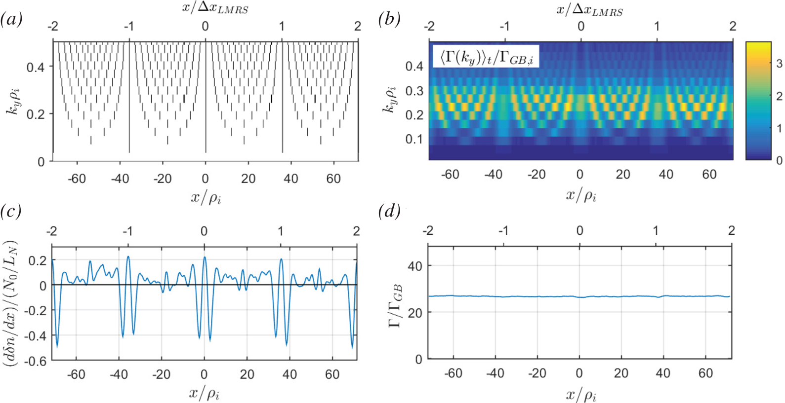
 $k_y$, etc.) and a misalignment around the higher-order MRSs, as shown in figure 4(a). This level of (mis)alignment of MRSs can be measured by their radial density, as shown in figure 12 in Dominski et al. (Reference Dominski, McMillan, Brunner, Merlo, Tran and Villard2017).
Other numerical parameters are as follows. In the  $k_x$ and
 $k_y$ Fourier spaces relative to the
 $x$ and
 $y$ directions, one considers
 $N_{k_x}$ and
 $N_{k_y}$ Fourier modes respectively. In real space, the simulation volume
 $L_x\times L_y\times L_z$ is discretised by
 $N_x\times N_y\times N_z$ equidistant grid points such that
 $N_x=N_{k_x}$ and
 $N_y=2N_{k_y}-1$. Note that by invoking the reality condition, only modes
 $k_y\geq 0$ are evolved in GENE. The parallel direction is treated in real space with
 $z \in [-L_z/2, +L_z/2[$. For our study, which, in particular, addresses a system size effect, it is essential to choose
 $L_z=2{\rm \pi}$, i.e. considering only one poloidal turn, for consistency with global geometries (Scott Reference Scott1998). The gyrocentre velocity space coordinates are
 $(v_{\parallel },\mu )$, where
 $\mu =mv_{\perp }^{2}/2B_0$ is the magnetic moment, and
 $v_\parallel$ and
 $v_{\perp }$ are the velocity components parallel and perpendicular to the magnetic field, respectively. For the parallel velocity direction one considers
 $v_\parallel \in [-v_{\parallel , \max }, +v_{\parallel , \max }]$ with a discretisation involving
 $N_{v_\parallel }$ equidistant grid points, whereas for the
 $\mu$ direction one considers
 $\mu \in [0, \mu _{\max }]$ with a discretisation involving
 $N_\mu$ grid points following the Gauss–Laguerre integration scheme.
3 Non-adiabatic passing electron dynamics leading to stationary zonal structures
This section presents a summary of relevant results from the articles (Dominski et al. Reference Dominski, Brunner, Görler, Jenko, Told and Villard2015, Reference Dominski, McMillan, Brunner, Merlo, Tran and Villard2017), which addressed certain effects of non-adiabatic passing electron dynamics on turbulent transport.
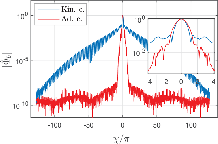
The non-adiabatic passing electron response leads to the generation of fine structures at MRSs that can be first studied in linear simulations. Figure 1 shows the envelope in the  $(x, z)$ plane of the electrostatic potential
 $\varPhi$ of the unstable linear ITG eigenmode with
 $k_y\rho _i=0.28$, considering either adiabatic or kinetic electron response, and for the set of physical parameters given in table 1. This is the same ITG case as considered by Dominski et al. (Reference Dominski, Brunner, Görler, Jenko, Told and Villard2015) and same numerical grid resolutions have been considered here. Although in both cases the modes are ballooned at
 $z=0$, one observes a fine radial structure at the corresponding MRS (positioned at the centre
 $x=0$ of the radial domain) only in the latter case. This is the result of the non-adiabatic passing electron response taking place at MRSs where the parallel wave number
 $k_\parallel \rightarrow 0$ (Chowdhury et al. Reference Chowdhury, Ganesh, Angelino, Vaclavik, Villard and Brunner2008; Dominski et al. Reference Dominski, Brunner, Görler, Jenko, Told and Villard2015). In the vicinity of MRSs, the condition for adiabatic electron response is violated as the phase velocity of the eigenmode parallel to the magnetic field becomes greater than the electron thermal velocity:
 $|\omega /k_\parallel |>v_{\textrm {th},e}$. These fine structures along the
 $x$ direction translate to a broad range of significant
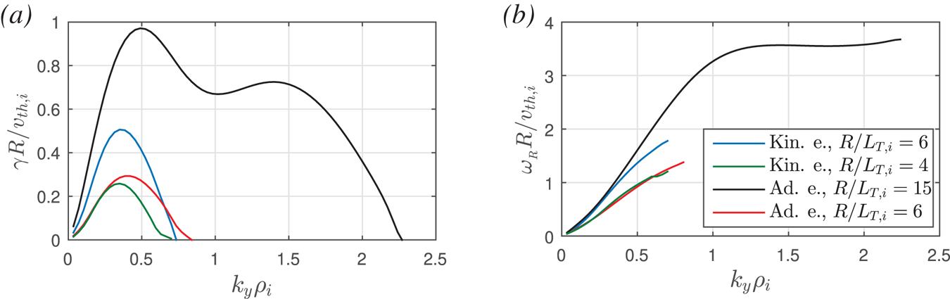
 $k_x$ Fourier modes, i.e. to a broad ballooning structure according to (2.18), which is referred to as the ‘giant electron tails’ in Hallatschek & Dorland (Reference Hallatschek and Dorland2005); see figure 2. No such broad tails in the ballooning structure are observed with adiabatic electrons. Figure 3 plots the
 $k_y$ spectrum of linear growth rates
 $\gamma$ and real frequencies
 $\omega _R$ of most unstable eigenmodes for the cases considered here. Note that
 $\omega _R>0$ corresponds in GENE convention to a mode propagating in the ion-diamagnetic direction, as expected for ITG instabilities.
Linear eigenmode with  $k_{x0}=0$ and
 $k_y\rho _i=0.28$, in the case of (a) adiabatic and (b) kinetic electron response. The
 $(x, z)$-dependence of the electrostatic potential
 $\varPhi$ in absolute value, weighted by the Jacobian
 $J |\varPhi |$, is shown.

Ballooning representation  $|\hat {\varPhi }_b(\chi )|$ of the electrostatic potential
 $\varPhi$ for the same linear eigenmode as in figure 1, showing both the case of kinetic (blue) and adiabatic (red) electrons. Inset: enlarged view near
 $\chi =0$.

(a) Linear growth rate  $\gamma$ and (b) real frequency
 $\omega _R$ in units of
 $v_{\textrm {th},i}/R$ as a function of
 $k_y\rho _i$. Adiabatic electron simulations with
 $R/L_{T,i}=6$ and
 $15$ are plotted in red and black, respectively. Kinetic electron simulations with
 $R/L_{T,i}=4$ and
 $6$ are plotted in green and blue, respectively.

Parameter set for non-linear simulations. The parameter  $k_{y, \min } = 2{\rm \pi} /L_y$ is scanned and takes the values
 $k_{y, \min }\rho _i\in \{0.14, 0.07, 0.035, 0.0175\}$, while
 $k_{y,\max }=k_{y, \min }N_y/2$ and
 $L_x=M/\hat {s}k_{y, \min }$ are kept constant. The values indicated in the table correspond to the particular case
 $k_{y, \min }\rho _i=0.035$. Asterisks indicate variables that vary during the
 $k_{y, \min }\rho _i$ scan. Here
 $v_{\textrm {th}, i} = \sqrt {T_i/m_i}$ denotes the ion thermal velocity and
 $B_{0, \textrm {axis}}$ for the magnetic field on axis.

The radial structures related to the non-adiabatic passing electron dynamics have been shown to persist in the non-linear turbulent regime, as discussed in Waltz et al. (Reference Waltz, Austin, Burrell and Candy2006) and Dominski et al. (Reference Dominski, Brunner, Görler, Jenko, Told and Villard2015, Reference Dominski, McMillan, Brunner, Merlo, Tran and Villard2017). Studies by Dominski et al. (Reference Dominski, Brunner, Görler, Jenko, Told and Villard2015, Reference Dominski, McMillan, Brunner, Merlo, Tran and Villard2017), based on both local (flux-tube) and global gyrokinetic simulations, have furthermore shown that, for each fluctuation mode with mode number  $k_y$, the corresponding MRSs act as radially localised transport channels. This is illustrated in figure 4(a,b). Radial regions with high (respectively, low) density of MRSs thus tend to lead to high (respectively, low) particle and heat diffusivities. Consequently, to ensure radially constant time-averaged total particle and heat fluxes, density and temperature gradients (driving the turbulence) become corrugated, steepening in regions with low density of MRSs and flattening in regions with high density of MRSs. See figure 4(c,d) where the time-averaged density gradient and particle flux are shown as a function
 $x$.
(a) Radial position of MRSs for each  $k_y$ mode, (b) radial dependence of contribution to time-averaged particle flux
 $\varGamma$ in gyro-Bohm units
 $\varGamma _{GB}=N_0v_{\textrm {th},i}(\rho _i/R)^{2}$ from each
 $k_y$ mode, (c) radial gradient of flux surface and time-averaged density fluctuation
 $\delta n$ normalised with respect to
 $N_0/L_N$ (positive/negative values correspond to flattening/steepening of profiles, respectively) and (d) radial profile of time-averaged total particle flux (summed over all
 $k_y$). All subplots correspond to kinetic electron simulation for the parameter set given in table 1, with
 $k_{y, \min }\rho _i=0.035$ and
 $R/L_{T,i}=6$. Ticks
 $x/{\rm \Delta} x_{\textrm {LMRS}}=\{-2,-1,0,1,2\}$ on the top axes denote the LMRSs.

Stationary  $E\times B$ shear flow layers associated with the time-averaged radial electric field are also observed (see figure 5 where the corresponding effective shearing rate as defined in (4.2) is plotted). This electric field component ensures the radial force balance with the pressure gradients related to the corrugation of density and temperature profiles (Waltz et al. Reference Waltz, Austin, Burrell and Candy2006). In §§ 5.3–5.5, it is shown that these stationary shear structures are actually driven by a contribution to the Reynolds Stress coming from the so-called self-interaction mechanism (Weikl et al. Reference Weikl, Peeters, Rath, Seiferling, Buchholz, Grosshauser and Strintzi2018).
(a) Effective shearing rate  $\omega _\textrm {eff}(x, t)$ plotted as a function of the radial position
 $x$ and time
 $t$, for the kinetic electron simulation with parameters as given in table 1,
 $k_{y, \min }\rho _i=0.035$ and
 $R/L_{T,i}=6$. (b) Solid blue line indicates the associated time-averaged component
 $\langle \omega _\textrm {eff}\rangle _t$, normalised by the corresponding maximum linear growth rate
 $\gamma _{\max }$, at each radial position
 $x$. The dashed blue line indicates the standard deviation
 $\textrm {SD}_t(\omega _\textrm {eff})(x) = [ \langle ( \omega _\textrm {eff} - \langle \omega _\textrm {eff}\rangle _t )^{2} \rangle _{t} ]^{1/2}$ in time, normalised by
 $\gamma _{\max }$. For comparison, results for
 $k_{y, \min }\rho _i=0.0175$ have been added in magenta.

4 Scan in  $k_{y, \min }\rho _i$ in ITG-driven turbulence: role of stationary and fluctuating components of zonal shear flows

Non-linear simulations have been carried out considering conditions of ITG-driven turbulence. Reference physical and numerical parameters for these simulations are summarised in table 1. The physical parameters are close to the CBC (Dimits et al. Reference Dimits, Bateman, Beer, Cohen, Dorland, Hammett, Kim, Kinsey, Kotschenreuther and Kritz2000), with background gradients slightly modified to eliminate unstable TEM and ETG modes. Compared with typical flux-tube runs, a high radial resolution is chosen (with radial grid points  $N_x=512$) to ensure that the dynamics at MRSs (separated by a radial distance
 ${\rm \Delta} x_{MRS}=1/\hat {s}k_y$ for a given
 $k_y$) is very well resolved, as discussed in detail in Dominski et al. (Reference Dominski, Brunner, Görler, Jenko, Told and Villard2015). In our work, this high
 $x$-resolution is all the more critical because the fine structures forming at the MRSs play an important role in the self-interaction mechanism, which is crucial to our study.
A scan in  $k_{y, \min }\rho _i$ is performed while keeping both
 $k_{y, \max }\rho _i$ and
 $L_x/\rho _i$ fixed. Successively halving
 $k_{y, \min }\rho _i$, the values
 $k_{y, \min }\rho _i = 0.14$,
 $0.07$,
 $0.035$ and
 $0.0175$ have been considered. Note that these values for
 $k_{y, \min }\rho _i$ span the typical range
 $10^{-2}\text {--}10^{-1}$ considered in practice when carrying out ion-scale flux-tube simulations. To keep
 $k_{y, \max }\rho _i$ fixed, the total number
 $N_y$ of
 $k_y$ modes must thus be doubled between consecutive runs, whereas to keep
 $L_x/\rho _i$ fixed, the number
 $M$ of LMRSs contained in the simulation box is halved. The parameter
 $M$ thus takes on the respective values
 $M= 16$,
 $8$,
 $4$ and
 $2$. The case
 $k_{y, \min }\rho _i=0.07$ is, in fact, equivalent to the ITG case already studied by Dominski et al. (Reference Dominski, Brunner, Görler, Jenko, Told and Villard2015).
Based on the relation  $k_{y,\min }\rho _i = (q_0a/r_0)\rho ^{*}$ (assuming that all toroidal modes are accounted for, so that
 $n_{\min }=1$) and for the typical mid-radius value
 $r_0/a=0.5$ and here considered
 $q_0=1.4$, one obtains
 $\rho ^{*} = 5.0\times 10^{-2}$,
 $2.5\times 10^{-2}$,
 $1.25\times 10^{-2}$ and
 $6.25\times 10^{-3}$. Note, for reference, that typical values for this parameter are
 $\rho ^{\star }\simeq 1\times 10^{-2}$ in a smaller machine such as the TCV tokamak,
 $\rho ^{\star }\simeq 3\times 10^{-3}$ in the DIII-D tokamak (Waltz Reference Waltz2005), whereas the projected values for ITER are still an order of magnitude smaller. To address how the results from the
 $k_{y, \min }\rho _i$ scan depend on whether one is near or far from marginal stability, the scan was repeated for a second ITG in both the adiabatic and kinetic electron cases. To this end, carrying out preliminary
 $R/L_{T_i}$ scans for
 $k_{y, \min }\rho _i = 0.035$, the non-linear (Dimits-shifted) critical temperature gradients
 $R/L_{T_i, \textrm {crit}}$ were first identified. For adiabatic electrons,
 $R/L_{T_i, \textrm {crit}}= 5.5$ was found, so that the reference case temperature gradient
 $R/L_{T_i} = 6$ is relatively near marginal stability and the second
 $k_{y, \min }\rho _i$ scan was, therefore, performed for
 $R/L_{\textrm {Ti}}= 15$ in this case, i.e. farther from marginal stability. For kinetic electrons,
 $R/L_{T_i, \textrm {crit}}= 3.5$, so that the reference case temperature gradient
 $R/L_{T_i} = 6$ is relatively far from marginal stability and the second
 $k_{y, \min }\rho _i$ scan was therefore performed for
 $R/L_{\textrm {Ti}}= 4$ in this case, i.e. nearer marginal stability.
To ensure that the simulations results are sound, convergence tests with respect to radial box size  $L_x$ and the numerical resolutions
 $N_z$,
 $N_{v_\|}$ and
 $N_\mu$ were carried out. A convergence test on
 $N_x$ had already been addressed in Dominski et al. (Reference Dominski, Brunner, Görler, Jenko, Told and Villard2015). Based on these tests, the turbulent heat and particle fluxes, as well as statistical properties of
 $E\times B$ shearing rates are estimated to be within
 ${\sim }10\,\%$ of their converged value. Benchmarking of the GENE results with the gyrokinetic code GS2 (Dorland et al. Reference Dorland, Jenko, Kotschenreuther and Rogers2000) was furthermore performed for a limited number of simulations. Although a reduced mass ratio is considered here, similar results have been obtained with the physical mass ratio of hydrogen
 $m_i/m_e=1836$.
First results from the  $k_{y, \min }\rho _i$ scan are now discussed. Given their importance in saturating ITG turbulence, particular attention will be given to the statistical properties of the shearing rate
 $\omega _{E\times B}$ associated with the zonal
 $E\times B$ flows. In fact, we consider the effective shearing rate
 $\omega _\textrm {eff}$, similar to that defined in Dominski et al. (Reference Dominski, Brunner, Görler, Jenko, Told and Villard2015). This rate is estimated as follows. One first defines the zonal
 $E\times B$ shearing rate experienced by the ions, which are the dominant instability drivers in the case of the here considered ITG turbulence:
 \begin{equation} \omega_{E\times B,\textrm{ion}}(x, t) = \frac{1}{B_0}\,\frac{\partial^{2}\langle\bar{\varPhi}\rangle_{y,z}}{\partial x^{2}}, \end{equation}
where the flux-surface average  $\langle \bar {\varPhi }\rangle _{y,z}$ provides the zonal component of
 $\bar {\varPhi }$ and involves both an average over
 $y$,
 $\langle \cdot \rangle _y = (1/L_y)\int _0^{L_y} \cdot \,\textrm {d}y$, and an average over
 $z$,
 $\langle \cdot \rangle _z = \int _{-{\rm \pi} }^{+{\rm \pi} }\cdot \,J^{xyz} \,\textrm {d}z/\int _{-{\rm \pi} }^{+{\rm \pi} } J^{xyz}\,\textrm {d}z$.
 $\bar {\varPhi }$ is the scalar potential gyroaveraged over the Maxwellian ion background velocity distribution. The shearing rate
 $\omega _{E\times B,\textrm {ion}}$ is then furthermore averaged over a small time window of width
 $\tau$, given that fluctuations that are very short-lived in time do not contribute effectively towards the zonal flow saturation mechanism (Hahm et al. Reference Hahm, Beer, Lin, Hammett, Lee and Tang1999), thus providing the effective shearing rate:
 \begin{equation} \omega_\textrm{eff}(x, t) = \frac{1}{\tau} \int_{t-\tau/2}^{t+\tau/2} \omega_{E\times B,\textrm{ion}}(x, t')\,\textrm{d}t'. \end{equation}
Here,  $\tau =1/\gamma _{\max }$ is considered, where
 $\gamma _{\max }$ is the growth rate of the most unstable linear mode.
As an illustration, the effective shearing  $\omega _\textrm {eff}(x, t)$ is plotted in figure 5(a) as a function of
 $x$ over the full flux-tube width
 $L_x$ and as a function of
 $t$ over the simulation time slice
 $50 < tv_\textrm {th, i}/R < 180$. Shown is the case with kinetic electrons,
 $R/L_{T_i}=6$ and
 $k_{y, \min }\rho _i = 0.035$. The radial profile for the time-averaged component
 $\langle \omega _\textrm {eff}\rangle _t(x)$, is shown in figure 5(b). For comparison, the same profile is also shown for the same physical parameters except for
 $k_{y, \min }\rho _i = 0.0175$.
The system average of the total effective shearing rate is plotted in figure 6(a) as a function of  $k_{y, \min }\rho _i$, considering a log–log scale. This average value is provided by the root-mean-square (RMS) estimate:
 \begin{equation} \textrm{RMS}_{x,t}(\omega_\textrm{eff}) = (\langle \omega_\textrm{eff}^{2}\rangle_{x,t})^{1/2}, \end{equation}
involving both a radial average,  $\langle \cdot \rangle _x = (1/L_x)\int _0^{L_x} \cdot \,\textrm {d}x$, and an average over the whole simulation time
 $t_\textrm {sim}$,
 $\langle \cdot \rangle _t = (1/t_\textrm {sim})\int _0^{t_\textrm {sim}} \cdot \,\textrm {d}t$. Figure 6(a) shows results for the scans carried out for the two respective temperature gradients
 $R/L_{T_i}$ considered for both adiabatic and kinetic electrons. The shearing rates have been normalised with respect to the value of
 $\gamma _{\max }$, which takes on different values for the four considered datasets (see figure 3). Normalised shearing values
 $\omega _\textrm {eff}/\gamma _{\max } \gtrsim 1$ can be considered as significant for saturating ITG-driven turbulence. Note that a straight system average
 $\langle \omega _\textrm {eff}(x,t) \rangle _{x,t}$ of the shearing rate would converge to zero over sufficiently long simulation time, which is why the RMS estimate (4.3) is considered. One notes that, over the considered range
 $10^{-2} \text {--}10^{-1}$ in
 $k_{y,\min }\rho _i$ values, the total effective shearing rate
 $\textrm {RMS}_{x,t}(\omega _\textrm {eff})$ decreases in all cases with decreasing
 $k_{y, \min }\rho _i$, i.e. with increasing machine size. However, significantly stronger scaling is observed for the scans with kinetic compared with adiabatic electrons. As can be seen from the log–log plot, the shearing rate appears to roughly scale as
 ${\sim }(k_{y, \min }\rho _i)^{\alpha }$,
 $\alpha >0$. This scaling is particularly evident for the kinetic electron case far from marginal stability (
 $R/L_{T_i}=6$), for which
 $\alpha \simeq 0.34$. Similar scaling is observed nearer marginal stability (
 $R/L_{T_i}=4$) as well. The adiabatic electron scans, however, show a weaker scaling with
 $\alpha \simeq 0.08$ for both
 $R/L_{T_i}=6$ and
 $R/L_{T_i}=15$.
Effective shearing rate  $\omega _\textrm {eff}$ associated with the zonal
 $E\times B$ flows, normalised to corresponding maximum linear growth rate
 $\gamma _{\max }$, as a function of
 $k_{y, \min }\rho _i$. Solid lines denote kinetic electron simulations for
 $R/L_{T,i}=4$ (green squares) and
 $6$ (blue circles), respectively. Dashed lines denote adiabatic electron simulations for
 $R/L_{T,i}=6$ (red triangles) and
 $15$ (black stars), respectively. Other parameters remain the same as in table 1. (a) System average of total shearing rate
 $\textrm {RMS}_{x,t}(\omega _\textrm {eff}) = (\langle \omega _\textrm {eff}^{2} \rangle _{x,t} )^{1/2}$. (b) Contribution from the stationary component,
 $\textrm {RMS}_{x}(\langle \omega _\textrm {eff}\rangle _t) = [\langle ( \langle \omega _\textrm {eff}\rangle _t )^{2} \rangle _{x} ]^{1/2}$. (c) Contribution from fluctuation component,
 $\textrm {SD}_{x,t}(\omega _\textrm {eff}) = [ \langle ( \omega _\textrm {eff} - \langle \omega _\textrm {eff}\rangle _t )^{2} \rangle _{x,t} ]^{1/2}$. All plots on a log–log scale.

Figure 7(a) plots, on a log–log scale, the time- and flux-tube-averaged radial ion heat flux  $Q_i$ as a function of
 $k_{y, \min }\rho _i$. Heat fluxes have been normalised to gyro-Bohm units
 $Q_{\textrm {GB},i} = n_{0, i}T_iv_{\textrm {th},i}(\rho _i/R)^{2}$. Results for all four considered datasets are again presented. Over the considered range of
 $k_{y, \min }\rho _i$, fluxes appear not to converge with respect to this parameter. This non-convergence is particularly striking for both adiabatic and kinetic electron simulations for the respective ITGs far from marginal stability. As can be seen from the log–log plot, in these cases one observes a scaling
 $Q_i/Q_{\textrm {GB},i} \sim (k_{y, \min }\rho _i)^{-\alpha }$,
 $\alpha >0$, with
 $\alpha = 0.45$ (kinetic electron,
 $R/L_{\textrm {Ti}}=6$) and
 $0.24$ (adiabatic electron,
 $R/L_{\textrm {Ti}}=15$).
(a) Log–log plot of the time-averaged and gyro-Bohm normalised ion heat flux  $Q_i$ as a function of
 $k_{y, \min }\rho _i$. Same cases as considered in figure 6. (b) Log–log plot of
 $k_y$ spectra of ion heat flux
 $Q_i$ for the kinetic electron runs with
 $R/L_{T,i}=6$ and
 $k_{y, \min }\rho _i=$ 0.0175 (magenta), 0.035 (blue), 0.07 (red) and 0.14 (green). Inset: enlarged view of the lin–lin plot near the peaks.

To provide insight into which wavelengths mainly contribute to the increasing heat flux as  $k_{y, \min }\rho _i$ decreases, the heat flux
 $k_y$ spectra is plotted in figure 7(b) for the set of simulations corresponding to the
 $k_{y, \min }\rho _i$ scan with kinetic electrons and
 $R/L_{T_i}=6$. Here
 $Q_{i,ky}$ is defined such that total heat flux
 $Q_i=\sum _{ky}Q_{i,ky}\,\textrm {d}k_y$, where
 $\textrm {d}k_y=k_{y, \min }$. One observes that all spectra present a peak at
 $k_y\rho _i\simeq 0.2$ and that the increase in heat flux as
 $k_{y, \min }\rho _i\to 0$ is not carried by the ever-smaller minimum wave numbers, but by the contributions of modes
 $0.07\le k_y\rho _i \le 0.35$ in the vicinity of the peak (contributing to at least
 $90\,\%$ of the heat flux), a range fully covered by all simulations, except for the largest considered
 $k_{y, \min }\rho _i=0.14$. Note that the inertial range (
 $k_y\rho _i\gtrsim 0.35$) remains essentially identical over all runs.
A priori, a straightforward explanation for the decreasing  $E\times B$ shearing rate leading to increased heat fluxes as
 $k_{y, \min }\rho _i$ decreases is the reduction in the radial density of stationary shear layers at LMRSs. Let us indeed recall that the distance between LMRSs is given by
 ${\rm \Delta} x_\textrm {LMRS} = 1/(k_{y, \min }\hat {s})$. Note as well the remarkable fact that the radial width and amplitude of the shear layers at LMRSs remains essentially invariant when varying
 $k_{y, \min }\rho _i$, as illustrated in figure 5(b). The contribution to the total shearing rate estimate (4.3) from the stationary component of the shearing rate profile
 $\langle \omega _\textrm {eff}\rangle _t(x)$ can be calculated by
 \begin{equation} \textrm{RMS}_{x}(\langle\omega_\textrm{eff}\rangle_t) = [ \langle ( \langle\omega_\textrm{eff}\rangle_t)^{2} \rangle_{x}]^{1/2}, \end{equation}
and has been plotted on a log–log scale as a function of  $k_{y, \min }\rho _i$ in figure 6(b). As expected, this system average of the stationary shearing rate profile decreases algebraically for kinetic electron simulations with decreasing
 $k_{y, \min }$, whereas for the adiabatic electron simulations there is no obvious dependence on
 $k_{y, \min }\rho _i$ as the mechanism developing the prominent fine stationary structures on
 $\langle \omega _\textrm {eff}\rangle _t(x)$ is absent in this case. However, this explanation for the increase of turbulent fluxes as a result of the decrease in the radial density of stationary zonal
 $E\times B$ shear layers is not satisfactory under closer scrutiny. This is made clear by the results presented in figure 8, where the radial correlation length of turbulent eddies
 $\lambda _x$ is plotted as a function of
 $k_{y, \min }\rho _i$ for the case with kinetic electrons and
 $R/L_{\textrm {Ti}}=6$. The radial correlation length is defined as
 $\lambda _x=\langle \lambda _x(y)\rangle _y$, with
 $\lambda _x(y)$ estimated as that smallest value of
 ${\rm \Delta} x$ for which the auto-correlation function
 $R({\rm \Delta} x,y)=\int \varPhi '^{*}(x-{\rm \Delta} x,y)\varPhi ' (x,y)\,\textrm {d}x$ is
 $1/e$ times its maximum value (this maximum is reached for
 ${\rm \Delta} x = 0$ and
 $e$ is the base of the natural logarithm).
 $\varPhi '(x,y)$ is the scalar potential evaluated at the outboard midplane, with the zonal (
 $k_y=0$) component removed:
 $\varPhi '(x,y)=\varPhi (x,y, z=0)-\langle \varPhi (x,y,z=0)\rangle _y$. This radial correlation length increases as
 $k_{y, \min }\rho _i$ decreases, but with a much weaker scaling (fit provides
 $\lambda _x/\rho _i \sim k_{y, \min }\rho _i^{-0.27}$ over the considered range
 $k_{y, \min }\rho _i = 10^{-2} \text {--} 10^{-1}$) than the increase of the distance
 ${\rm \Delta} x_\textrm {LMRS}/\rho _i\sim (k_{y, \min }\rho _i)^{-1}$ between the main stationary shear layers located at LMRSs. Below a sufficiently small value of
 $k_{y, \min }\rho _i$, one thus clearly has
 $\lambda _x \ll {\rm \Delta} x_\textrm {LMRS}$. That is, the turbulent eddies are getting actively sheared and broken in between low-order MRSs where the stationary zonal shear flows are insignificant. The stationary shear layers are therefore not expected to play a major role in the saturation of turbulence as
 $k_{y, \min }\rho _i\to 0$. We therefore conclude that as
 $k_{y, \min }\rho _i\to 0$, the saturation of turbulence through the break-up of turbulent eddies is mainly to be attributed to the fluctuating component of zonal flows. This is discussed in detail in the following.
Blue circles denote the radial correlation length  $\lambda _x$ of turbulent eddies in units of
 $\rho _i$ as a function of
 $k_{y, \min }\rho _i$ for kinetic electron simulations and
 $R/L_{T,i}=6$ (all parameters as given in table 1). Magenta asterisks correspond to results obtained with the same parameters except for a decreased radial resolution (by a factor
 $4$), which enabled us to carry out runs with
 $k_{y, \min }\rho _i$ values as low as
 ${\sim }5\times 10^{-3}$ (these simulations are discussed in more detail in relation with figure 18). Distance
 ${\rm \Delta} x_{\textrm {LMRS}}=1/(k_{y, \min }\hat {s})$ between LMRSs is plotted with black squares.

The time-dependent component (as opposed to the stationary component) of the  $E\times B$ zonal flow and associated shearing rate thus appears to control the saturation of turbulence and related flux levels between LMRSs. An estimate for the amplitude of this fluctuating part of the shearing rate is provided by computing the radial profile of the standard deviation
 $\textrm {SD}_t(\omega _\textrm {eff})$ of
 $\omega _\textrm {eff}$ around the stationary component
 $\langle \omega _\textrm {eff}\rangle _t$:
 \begin{equation} \textrm{SD}_{t}(\omega_\textrm{eff})(x) = [\langle (\omega_\textrm{eff} - \langle\omega_\textrm{eff}\rangle_t)^{2}\rangle_{t}]^{1/2}. \end{equation}
The radial dependence of  $\textrm {SD}_{t}(\omega _\textrm {eff})$ has been added to figure 5(b) for the cases with kinetic electrons,
 $R/L_{T_i}=6$ and both
 $k_{y, \min }\rho _i = 0.035$ and
 $k_{y, \min }\rho _i = 0.0175$. Based on figure 5(b), it appears that the fluctuating part of the shearing rate remains essentially constant across the radial extent of the system. Furthermore, its amplitude for the considered values of
 $k_{y, \min }\rho _i$ still remains significant, i.e. larger than
 $\gamma _{\max }$, and of the same order as the maximum amplitude of the time-averaged
 $\langle \omega _{E\times B}\rangle _t$ structures. A decrease of the fluctuating component with decreasing
 $k_{y, \min }\rho _i$ is also observed. This is summarised in figure 6(c), where the radial average of the fluctuating component, estimated by
 \begin{equation} \textrm{SD}_{x,t}(\omega_\textrm{eff}) = [ \langle ( \omega_\textrm{eff} - \langle\omega_\textrm{eff}\rangle_t)^{2}\rangle_{x,t}]^{1/2}, \end{equation}
has been plotted. Although  $\textrm {SD}_{x,t}(\omega _\textrm {eff})$ decreases with
 $k_{y, \min }\rho _i$ in both adiabatic and kinetic electron simulations, the scaling is much stronger in the latter case. For instance, in the considered range of
 $k_{y, \min }\rho _i$,
 $\textrm {SD}_{x,t}(\omega _\textrm {eff})\sim (k_{y, \min }\rho _i)^{\alpha }$, where
 $\alpha =0.08$ for the case with adiabatic electrons at
 $R/L_{\textrm {Ti}}=15$ whereas
 $\alpha =0.32$ for the case with kinetic electrons at
 $R/L_{\textrm {Ti}}=6$.
Note that according to the definitions (4.3), (4.4) and (4.6), one has
 \begin{equation} [\textrm{RMS}_{x,t}(\omega_\textrm{eff})]^{2} = [ \textrm{RMS}_{x}(\langle\omega_\textrm{eff}\rangle_t)]^{2} + [ \textrm{SD}_{x,t}(\omega_\textrm{eff}) ]^{2}. \end{equation}
The decrease of both the fluctuation level of the shearing rate, shown in figure 6(c), along with the decrease in the density of stationary shearing layers at LMRSs, reflected by figure 6(b), thus provides a more complete picture of the decrease in the total system average of the shearing rate  $\omega _\textrm {eff}$ as
 $k_{y,\min }\rho _i$ decreases, shown in figure 6(a). Although the reason for the decrease in the contribution to the shearing rate from stationary zonal flows has already been discussed and is relatively obvious, the reason for the decrease of the contribution from fluctuating zonal flows is not. To explain the latter, it is necessary to understand and analyse the different mechanisms driving the zonal flows. This is done in the following section.
5 Analysing zonal flow drive
In this section, the drive of zonal flows via the two main mechanisms, the modulational instability and self-interaction, are studied. In particular, the statistical properties of these different zonal flow drives are analysed using various diagnostics techniques, with the primary objective of understanding why the fluctuating zonal flow levels decrease with decreasing  $k_{y,\min }\rho _i$ as seen in figure 6(c).
To ensure a systematic study, this section has been organised as follows. To start, it is essential to identify the physical quantity (or quantities) representing the drive of zonal flows ( $\sim$ modes
 $k_{y}\rho _i=0$) from turbulence (
 $\sim$ modes
 $k_{y}\rho _i\neq 0$). In § 5.1, it is found that Reynolds stress can be used as a convenient proxy for quantifying the drive of zonal flows. The two main mechanisms driving zonal flows are then discussed in the following two subsections: a summary of the well-known modulational instability mechanism is given in § 5.2, followed by a detailed description of the self-interaction mechanism in § 5.3. These two mechanisms and the nature of their drives are illustrated first in a simple non-linear set-up, referred to as the ‘reduced simulations’, in § 5.4. This is followed by providing the evidence for self-interaction and modulational instability in full turbulence simulations, discussed in §§ 5.5 and 5.6, respectively. In the latter subsection, using a bicoherence-like analysis and an estimate of the correlation between the different
 $k_y$ contributions to Reynolds stress, it is shown that the drive of zonal flows via self-interaction from each
 $k_y$ are essentially incoherent and decorrelated, unlike that via modulational instability. This result will then be used in the following § 6, to show how such a decorrelated drive could explain the observed decrease in fluctuating zonal flow levels with decreasing
 $k_{y,\min }\rho _i$.
5.1 Reynolds stress as a proxy for the drive of zonal flows
Zonal flows are linearly stable and are driven by turbulence through the quadratic  $E \times B$ non-linearity appearing in the gyrokinetic equation. To better understand their evolution, we analyse the properties of Reynolds stress (Diamond et al. Reference Diamond, Itoh, Itoh and Hahm2005), more exactly the off-diagonal component
 $\langle \tilde {V}_x\tilde {V}_\chi \rangle$ of the Reynolds stress tensor resulting from the combination of fluctuating
 $E\times B$ flow components in the radial and poloidal directions. We justify in the following that this Reynolds stress can be considered as a valid proxy of the zonal flow drive (Weikl et al. Reference Weikl, Peeters, Rath, Seiferling, Buchholz, Grosshauser and Strintzi2018). By analysing Reynolds stress we will be able to identify the different possible mechanisms driving zonal flows, their statistical properties and relative importance.
We start by considering an approximate evolution equation for the shearing rate  $\omega _{E\times B}$ associated with the
 $E\times B$ zonal flows. As shown by Parra & Catto (Reference Parra and Catto2009) and Abiteboul et al. (Reference Abiteboul, Garbet, Grandgirard, Allfrey, Ghendrih, Latu, Sarazin and Strugarek2011); Abiteboul (Reference Abiteboul2012), such an equation can be obtained from the radial conservation equation for the total gyrocentre charge density, which, in turn, is derived by taking the appropriate velocity moment and flux-surface average of the gyrokinetic equation. The approach in Abiteboul (Reference Abiteboul2012) has been considered here, but starting from the gyrokinetic equation in the limit of the local (flux-tube) delta-f model rather than the global full-f model considered by Abiteboul (Reference Abiteboul2012). Furthermore, assuming the electrostatic limit, invoking
 $m_e/m_i\ll 1$, and making use of the quasi-neutrality equation in the long-wavelength approximation (final result thus valid only to second order in
 $k_\perp \rho _i$), leads to a relation that can be interpreted as a generalised vorticity equation:
 \begin{equation} \frac{\partial }{\partial t} (\varOmega+\varPi) = \frac{\partial^{2}}{\partial x^{2}} (\mathcal{R} + \mathcal{P}) + \frac{\partial}{\partial x}\mathcal{N}. \end{equation}
One identifies on the left-hand side of (5.1) the generalised vorticity term  $\varOmega +\varPi$, composed of the actual vorticity associated with zonal flows and closely related to the zonal flow shearing rate
 $\omega _{E\times B}$ (by neglecting the
 $z$ dependence of
 $B_0$ and
 $g^{xx}\simeq 1$),
 \begin{equation} \varOmega = n_{0,i}m_i \frac{\partial^{2}}{\partial x^{2}} \left\langle \frac{g^{xx}}{B_0^{2}}\,\varPhi \right\rangle_{yz} \simeq \frac{n_{0, i}m_i}{B_0}\,\omega_{E\times B}, \end{equation}
as well as a perpendicular pressure term, related to lowest-order finite ion Larmor radius effects,
 \begin{equation} \varPi =\frac{m_i}{2q_i} \frac{\partial^{2}}{\partial x^{2}} \left \langle \frac{g^{xx}}{B_0^{2}}\, P_{\perp,i} \right \rangle_{yz}, \end{equation}
with the fluctuating part of the perpendicular ion gyrocentre pressure  $P_{\perp ,i}$ expressed in terms of the corresponding gyrocentre distribution fluctuation
 $\delta f_i$,
 \begin{equation} P_{\perp,i} = \int \mu B_0\delta f_i\,\textrm{d}^{3}v. \end{equation}
On the right-hand side of (5.1) one identifies the second radial derivative of a term  $\mathcal {R}=(n_{0,i}m_i/\mathcal {C})\textrm {RS}$, proportional to the Reynolds stress component
 $\textrm {RS}$ driving zonal flows:
 \begin{equation} \textrm{RS} = \left\langle \frac{1}{B_0^{2}}\frac{\partial \varPhi}{\partial y} \left( g^{xx}\frac{\partial \varPhi}{\partial x} + g^{xy}\frac{\partial \varPhi}{\partial y} \right) \right\rangle_{yz}. \end{equation}
This Reynolds stress term also has a finite Larmor radius correction term  $\mathcal {P}$, again expressed in terms of
 $P_{\perp ,i}$:
 \begin{equation} \mathcal{P} = \frac{m_i}{2q_i\mathcal{C}} \left\langle \frac{1}{B_0^{2}} \left( g^{xx} \frac{\partial\varPhi}{\partial x} \frac{\partial P_{\perp,i}}{\partial y} + 2g^{xy}\, \frac{\partial \varPhi}{\partial y} \frac{\partial P_{\perp,i}}{\partial y} + g^{xx} \frac{\partial \varPhi}{\partial y} \frac{\partial P_{\perp,i}}{\partial x} \right) \right\rangle_{yz}. \end{equation}
The last contribution on the right-hand side of (5.1) is the radial derivative of the so-called neoclassical term  $\mathcal {N}$, related to both curvature and
 $\boldsymbol {\nabla } B$ drifts:
 \begin{equation} \mathcal{N} = -\sum_\textrm{species} \frac{2{\rm \pi}\mathcal{C}}{m} \left\langle \gamma_2 \frac{\partial B_0}{\partial z} \int \textrm{d}v_\parallel \,\textrm{d}\mu\,\frac{mv_\parallel^{2} + \mu B_0}{B_0^{2}} \left( \delta f + \frac{q\,\bar{\varPhi}}{T_0} f_0 \right) \right\rangle_{yz}, \end{equation}
with  $f_0$ the Maxwellian background distribution,
 $\gamma _2{=}g^{xx}g^{yz}-g^{xy}g^{xz}$ and the constant
 $\mathcal {C}{=}B_0/|\boldsymbol {\nabla } x\times \boldsymbol {\nabla } y|$.
The different terms appearing in (5.1) can be monitored as a diagnostic along a gyrokinetic simulation. For the purpose of verification, this diagnostic was first applied to simple test cases, including the Rosenbluth–Hinton problem (Rosenbluth & Hinton Reference Rosenbluth and Hinton1998) addressing the linear dynamics of zonal fluctuations (in this case, only the linear neoclassical term contributes on the right-hand side of (5.1)), as well as the non-linear decay of an initially single unstable eigenmode (as discussed in § 5.4). For these simple tests, only longer wavelength modes were considered, so as to stay well within the limit  $k_\perp \rho _i\ll 1$ assumed for the derivation of relation (5.1).
After this successful initial verification phase, the terms appearing in (5.1) were monitored and compared for the fully developed turbulence simulations studied in this paper, considering the reference gradient case  $R/L_{T,i}=6$. To validate Reynolds stress as a good proxy for the drive of zonal flows, the correlation between
 $\varOmega \sim \omega _{E\times B}$ and the two non-linear driving terms
 $\partial ^{2}\mathcal {R}/\partial x^{2}$ and
 $\partial ^{2}\mathcal {P}/\partial x^{2}$ in (5.1) was estimated over these simulations. To this end, the following correlation estimator between two observables
 $a$ and
 $b$, functions of the radial variable
 $x$ and time
 $t$, was applied:
 \begin{equation} \textrm{Corr}(a,b) = \frac{\sigma_{x,t}(a, b)}{\sigma_{x,t}(a)\sigma_{x,t}(b)} = \frac{ \langle (a-\langle a\rangle_{x,t}) (b-\langle b\rangle_{x,t}) \rangle_{x,t}} {\sqrt{\langle(a-\langle a\rangle_{x,t})^{2}\rangle_{x,t}} \sqrt{\langle(b-\langle b\rangle_{x,t})^{2}\rangle_{x,t}}}. \end{equation}
Significant correlation estimates were obtained in this way between  $\varOmega$ and the Reynolds stress drive term
 $\partial ^{2}\mathcal {R}/\partial x^{2}$. Correlation values were found to increase further by considering only the longer wavelength contributions, achieved by filtering out
 $|k_x|\rho _i > 0.5$ and
 $|k_y|\rho _i>0.5$ Fourier modes from the signals. This is in agreement with the long-wavelength approximation assumed for deriving (5.1). The positive correlation values
 $\textrm {Corr} = 0.77$ and
 $0.37$ were obtained in this way between
 $\varOmega$ and
 $\partial ^{2}\mathcal {R}/\partial x^{2}$ for the adiabatic and kinetic electron turbulence simulations, respectively, whereas the correlation between
 $\varOmega$ and
 $\partial ^{2}\mathcal {P}/\partial x^{2}$ provided the values
 $\textrm {Corr} = 0.75$ and
 $0.40$, respectively. These results validate considering the Reynolds stress term
 $\partial ^{2}\textrm {RS}/\partial x^{2}$ as a proxy for the drive of zonal flow shear
 $\omega _{E\times B}$.
In the following, it will be insightful to consider the contributions from different  $k_y$ Fourier modes components of the fluctuating fields to the Reynolds stress term
 $\textrm {RS}$. Relation (5.5) for
 $\textrm {RS}$ can indeed be written as a sum over
 $k_y$:
 \begin{equation} \textrm{RS}(x, t) = \sum_{k_y > 0} \widehat{\textrm{RS}}_{k_y}(x, t), \end{equation}
with the contribution from the  $k_y$ Fourier mode
 $\hat \varPhi _{k_y}(x, z, t) = ({1}/{L_y}) \int _0^{L_y} \varPhi \exp (-{\mathrm i}k_yy)\,\textrm {d}y$ given by
 \begin{equation} \widehat{\textrm{RS}}_{k_y}(x, t) = 2\,{Re} \left[ \left\langle \frac{1}{B_0^{2}}\,k_y\hat{\varPhi}_{k_y} \left( g^{xx}\textrm{i}\,\frac{\partial \hat{\varPhi}_{k_y}^{\star}}{\partial x} + g^{xy} k_y \hat{\varPhi}_{k_y}^{\star} \right) \right\rangle_z \right], \end{equation}
having invoked the reality condition  $\hat \varPhi _{-k_y}=\hat \varPhi _{k_y}^{\star }$. Considering as well the
 $k_x$ Fourier mode decomposition of
 $\varPhi$, each of these
 $k_y$ contributions can also be written as follows:
 \begin{equation} \widehat{\textrm{RS}}_{k_y}(x, t) = 2\,{Re} \left\{ \sum_{k_x, k_x''} \left\langle \frac{1}{B_0^{2}}\,k_y \left( g^{xx} k_x'' + g^{xy} k_y \right)\hat{\varPhi}_{k_x,k_y} \hat{\varPhi}_{k_x'',k_y}^{\star} \right\rangle_z \exp[\textrm{i}(k_x-k_x'')x] \right\}, \end{equation}
illustrating the drive of zonal modes  $(k_x'=k_x-k_x'', 0)$ through non-linear interaction between Fourier modes
 $(k_x, k_y)$ and
 $(k_x'', k_y)$, extensively discussed in §§ 5.2 and 5.3.
For the study carried out in this paper, it is essential to understand how different drift modes may non-linearly interact to drive zonal flows via Reynolds stress. To start, we recall in the next subsection the basic mechanism underlying the drive of zonal flows in a simple shearless slab system before considering the more complex case of direct interest to us, i.e. of a sheared toroidal system.
5.2 Modulational instability in shearless slab system
The drive of zonal flows by microturbulence has been studied extensively in the literature considering a simple slab-like plasma confined by a uniform, shearless magnetic field. Such a system was in particular addressed in the original work by Hasegawa & Mima (Reference Hasegawa and Mima1978), where a cold fluid model was assumed for ions and an adiabatic response for electrons. In this model, choosing an orthogonal Cartesian coordinate system  $(x, y, z)$, the magnetic field is aligned along
 $z$,
 $\boldsymbol {B} = B\boldsymbol {e}_z$ and the background density inhomogeneities along
 $x$,
 $\boldsymbol {\nabla } n_0 = (\textrm {d} n_0/\textrm {d}x)\boldsymbol {e}_x$. The corresponding well-known model equation for the non-linear evolution of the electrostatic potential
 $\varPhi$ associated to the fluctuating fields describes the essentially two-dimensional drift wave turbulence in the
 $(x, y)$ plane perpendicular to the magnetic field. This model equation led to a first understanding of the generation of zonal flows along
 $y$, i.e. in the direction both perpendicular to
 $\boldsymbol {B}$ and the direction of inhomogeneity. The emergence of such large-scale flows can in particular be explained as the result of an anisotropic inverse cascade of energy related to the conservation of energy and enstrophy in the two-dimensional turbulence. The emergence of zonal flows can also be understood at the level of elementary non-linear processes as recalled in the following.
In a shearless slab system, the spatial dependence of linear eigenmodes are given by a single Fourier mode  $\varPhi (x, y)\sim \varPhi _{{{\boldsymbol {k}}}}\exp (\textrm {i}{{\boldsymbol {k}}}\boldsymbol {\cdot }{{\boldsymbol {x}}})$, with
 ${{\boldsymbol {x}}} = x\,{{\boldsymbol {e}}}_x+y\,{{\boldsymbol {e}}}_y$ and
 ${{\boldsymbol {k}}} = k_x{{\boldsymbol {e}}}_x+k_y{{\boldsymbol {e}}}_y$. The corresponding time dependence is of the form
 $\sim \exp (-\textrm {i}\omega _{{\boldsymbol {k}}}t)$, with
 $\omega _{{\boldsymbol {k}}}$ the eigenfrequency of the mode. In the simple Hasegawa–Mima model, one has
 $\omega _{{\boldsymbol {k}}} = k_y\,v_d/(1+k^{2})$, with
 ${{\boldsymbol {v}}}_d = -(T_e/eB)(\textrm {d}\log n_0/\textrm {d}x)\, {{\boldsymbol {e}}}_y$ these eigenmodes result from the quadratic non-linearity in the Hasegawa–Mima equation, related to the
 ${{\boldsymbol {v}}}_{E\times B} = (-\boldsymbol {\nabla }\varPhi \times {{\boldsymbol {B}}})/B^{2}$ drift. The elementary non-linear interaction thus involves a triplet of Fourier modes
 ${{\boldsymbol {k}}}$,
 ${{\boldsymbol {k}}}'$,
 ${{\boldsymbol {k}}}''$ verifying the wave vector matching condition
 ${{\boldsymbol {k}}} = {{\boldsymbol {k}}}'+{{\boldsymbol {k}}}''$, where each of the modes, e.g.
 ${{\boldsymbol {k}}}$, is coupled to the two others,
 ${{\boldsymbol {k}}}'$ and
 ${{\boldsymbol {k}}}''$ in this case. In case of frequency matching
 $\omega _{{\boldsymbol {k}}}\simeq \omega _{{{\boldsymbol {k}}}'}+\omega _{{{\boldsymbol {k}}}''}$ and under the condition
 $k' < k < k''$, one can have a resonant decay of mode
 ${{\boldsymbol {k}}}$, i.e. a transfer of energy from this mode, into the daughter modes
 ${{\boldsymbol {k}}}'$ and
 ${{\boldsymbol {k}}}''$. This basic process is referred to as the resonant three-wave interaction mechanism. One can furthermore show that in the case where mode
 ${{\boldsymbol {k}}}$ represents a drift wave, i.e. typically with
 $|k_y| \gg |k_x|$, the decay happens preferentially (meaning with a higher growth rate of decay) if one of the daughter wave vectors, e.g.
 ${{\boldsymbol {k}}}'$, is (nearly) aligned along the
 $x$ direction,
 $|k_x'| \gg |k_y'|$ (Hasegawa et al. Reference Hasegawa, Maclennan and Kodama1979). The
 $E\times B$ flow associated with the daughter mode
 ${{\boldsymbol {k}}}'$ is then obviously along
 $y$, thus explaining the emergence of zonal flows in this direction. Such a mode with vector aligned along the direction of inhomogeneity
 ${{\boldsymbol {e}}}_x$ is thus referred to as a zonal mode.
Let us still further consider the decay of a pump drift wave  ${{\boldsymbol {k}}} = (k_x, k_y)$,
 $k_y\neq 0$, into a zonal mode
 ${{\boldsymbol {k}}}'= (k_x', 0)$ and the second daughter wave
 ${{\boldsymbol {k}}}'' = {{\boldsymbol {k}}}-{{\boldsymbol {k}}}' = (k_x-k_x', k_y)$, itself a drift wave. The non-linear interaction between the two drift waves
 ${{\boldsymbol {k}}}$ and
 ${{\boldsymbol {k}}}''$ thus provides the drive to the zonal mode
 ${{\boldsymbol {k}}}'$ via the Reynolds stress
 $\textrm {RS}$ discussed in § 5.1, whereas the non-linear coupling between the original drift wave
 ${{\boldsymbol {k}}}$ and zonal mode
 ${{\boldsymbol {k}}}'$, leading to the growth of the daughter drift wave
 ${{\boldsymbol {k}}}''$, actually represents the shearing of the drift mode
 ${{\boldsymbol {k}}}$ by the zonal flows associated with
 ${{\boldsymbol {k}}}'$.
Variations to the simple Hasegawa–Mima model have been considered in the literature. In particular, the enhanced Hasegawa–Mima model (Krommes & Kim Reference Krommes and Kim2000; Gallagher et al. Reference Gallagher, Hnat, Connaughton, Nazarenko and Rowlands2012) accounts for the fact that the adiabatic electron response is inhibited for magnetic surface-averaged fluctuations, i.e. modes  ${{\boldsymbol {k}}}$ with
 $k_y=0$, in other words zonal modes, which leads them to having a reduced effective inertia compared with standard drift waves with
 $k_y\neq 0$. This effect results in an amplification of the decay rates of drift waves into zonal modes and, thus, to an enhancement of corresponding energy transfer.
A further refinement to the basic driving mechanism of zonal flows is obtained by accounting for the fact that given an initial large-amplitude drift mode  $\boldsymbol {k}$, decaying into a zonal mode
 $\boldsymbol {k}'$, both triplet interactions
 $[\boldsymbol {k}, \boldsymbol {k}', \boldsymbol {k}'' = \boldsymbol {k}-\boldsymbol {k}']$ and
 $[\boldsymbol {k}, -\boldsymbol {k}', \boldsymbol {k}''' = \boldsymbol {k}+\boldsymbol {k}']$ may be simultaneously resonant, i.e.
 $\omega _{\boldsymbol {k}} \simeq \omega _{\boldsymbol {k}'}+\omega _{\boldsymbol {k}''}$ and
 $\omega _{\boldsymbol {k}} \simeq -\omega _{\boldsymbol {k}'}+\omega _{\boldsymbol {k}'''}$. This coupled pair of three-wave interactions leads to an effective four-wave interaction involving modes
 $\boldsymbol {k}$,
 $\boldsymbol {k}'$,
 $\boldsymbol {k}''$ and
 $\boldsymbol {k}'''$, referred to as the modulational instability mechanism (Gallagher et al. Reference Gallagher, Hnat, Connaughton, Nazarenko and Rowlands2012).
An important point to emphasise is that, in both the case of the simple resonant three-wave interaction or the more general modulational instability, resonant coupling between the initial large-amplitude (pump) drift mode  ${{\boldsymbol {k}}}=(k_x, k_y\neq 0)$ and a zonal mode
 ${{\boldsymbol {k}}}'=(k_x', k_y'=0)$ is established via either one sideband
 ${{\boldsymbol {k}}}''={{\boldsymbol {k}}}-{{\boldsymbol {k}}}'$ or, respectively, two sidebands
 ${{\boldsymbol {k}}}''$ and
 ${{\boldsymbol {k}}}'''={{\boldsymbol {k}}}+{{\boldsymbol {k}}}'$, where all of these Fourier modes are linearly decoupled from each other. As a result, in the situation where in addition to the pump drift mode
 ${{\boldsymbol {k}}}$, the zonal mode
 ${{\boldsymbol {k}}}'$ itself already has a finite initial amplitude and a well-defined phase, the other daughter waves
 ${{\boldsymbol {k}}}''$ (and
 ${{\boldsymbol {k}}}'''$) are free to adapt their phases to ensure a resonant interaction and, thus, an efficient energy transfer from the pump to the zonal mode, resulting in the further amplification of this zonal mode. In fact, a finite-amplitude zonal mode can stimulate the decay of multiple non-zonal modes, thus leading to coherent (as a result of the frequency matching involved) and therefore correlated contributions from these non-zonal modes to the Reynolds stress drive of the zonal mode.
Under realistic conditions, multiple elementary mechanisms such as those discussed previously (resonant three-wave interaction/modulational instability) happen both simultaneously and successively in time, leading to an expanding set of Fourier modes, and ultimately to a fully developed turbulent spectrum.
5.3 Self-interaction mechanism in sheared toroidal system
As in the shearless slab geometry, in the case of a tokamak system, i.e. based on a sheared axisymmetric toroidal magnetic geometry, which is of main interest to our study, the modulational instability involving resonant three-wave interactions remains an essential driving mechanism of zonal flows (Chen et al. Reference Chen, Lin and White2000). In a tokamak, however, one must distinguish another form of the non-linear interaction leading to the drive of zonal modes. This mechanism, referred to as self-interaction, is specific to systems presenting magnetic shear and is explained in the following.
As already discussed in § 2, parallel boundary conditions lead to the linear coupling of  $k_x$ Fourier modes. In particular, according to (2.16), the electrostatic potential field
 $\varPhi _{L}$ of a linear microinstability eigenmode with fixed
 $k_{x0}$ and
 $k_y\neq 0$ is composed of Fourier modes
 $\hat {\varPhi }_{k_{x0} + p2{\rm \pi} k_y\hat {s},k_y}$,
 $p\in \mathbb {Z}$. The spatial dependence of the corresponding eigenmode structure is thus given by
 \begin{equation} \varPhi_{L}(x, y, z) = \tilde{\varPhi}_{k_{x0},k_y}(x,z)\exp(\textrm{i}k_yy) + \textrm{c.c.}, \end{equation}
where  $\textrm {c.c.}$ denotes the complex conjugate (considered here to ensure that
 $\varPhi _L$ is real-valued, essential for computing the quasi-linear estimate in (5.14)), and with the complex-valued
 $(x,z)$-dependent envelope given by
 \begin{equation} \tilde{\varPhi}_{k_{x0},k_y}(x,z) = \sum_{p=-\infty}^{+\infty} \hat{\varPhi}_{k_{x0} + p2{\rm \pi} k_y\hat{s},k_y}(z) \exp[\textrm{i}(k_{x0} + p2{\rm \pi} k_y\hat{s})x]. \end{equation}
These linearly coupled  $k_x$ Fourier modes, all having same
 $k_y$, drive the zonal modes
 $(k_x', 0)$, with
 $k_x'=p'2{\rm \pi} k_y\hat {s}$,
 $p'\in \mathbb {Z}$, forming a set of harmonics. Indeed, any two Fourier modes
 $\hat {\varPhi }_{k_{x0} + p2{\rm \pi} k_y\hat {s}, k_y}$ and
 $\hat {\varPhi }_{k_{x0} + p''2{\rm \pi} k_y\hat {s},k_y}$ composing the physical eigenmode will drive, via three Fourier mode coupling, the zonal mode
 $\hat {\varPhi }_{p'2{\rm \pi} k_y\hat {s},0}$ with
 $p'=p-p''$ (see (5.11)). Note that this drive of zonal modes is via the same quadratic non-linearity in the gyrokinetic equation related to
 $E\times B$ drifts as that driving zonal modes through the modulational instability, but in this case involving Fourier modes that are already linearly coupled to each other.
Assuming that the relative phases between the Fourier modes  $\hat {\varPhi }_{k_{x, 0} + p2{\rm \pi} k_y\hat {s},k_y}$ remains set by the linear coupling, even during the non-linear turbulent evolution (to what extent this assumption holds is validated in § 5.5), the phases of the associated contributions to Reynolds stress driving the zonal modes is fixed. This translates in direct space to an essentially fixed periodic radial dependence (with period
 ${\rm \Delta} x_\textrm {MRS} = 1/k_y\hat {s}$ corresponding to the distance between MRSs) of the contribution to Reynolds stress through this self-interaction mechanism from a given
 $k_y$ eigenmode, the overall magnitude of this contribution obviously varying in time as the amplitude of the eigenmode evolves. This is a critical difference compared with the drive of zonal modes
 ${{\boldsymbol {k}}}'$ through the modulational instability discussed in § 5.2, where the relative phases between the pump mode
 ${{\boldsymbol {k}}}$ and sidebands
 ${{\boldsymbol {k}}}''$,
 ${{\boldsymbol {k}}}'''$ are free to adapt to enable a coherent (i.e. in phase) drive of a given zonal mode.
Figure 9 plots the quasi-linear estimates of this self-interaction contribution to the Reynolds stress drive term  $\partial ^{2}\textrm {RS}/\partial x^{2}$ from the linear eigenmode with
 $k_{x0}=0$,
 $k_{y}\rho _i = 0.28$ and
 $R/L_{T_i} =6$, whose ballooning structures are given in figure 2, considering both the case of kinetic and adiabatic electron response. These results are obtained by inserting the corresponding eigenmode structure (5.12) into relations (5.10) and (5.11), leading to the Reynolds stress contribution denoted by
 $\widetilde{\textrm {RS}}_{k_{x0},k_y}(x)$:
 \begin{align} \widetilde{\textrm{RS}}_{k_{x0},k_y}(x) & = \textrm{RS}[\varPhi_L] = \widehat{\textrm{RS}}_{k_y}[\tilde{\varPhi}_{k_{x0}, k_y}] \nonumber\\ & = 2\,{Re} \left[ \left\langle \frac{1}{B_0^{2}}\,k_y\tilde{\varPhi}_{k_{x0}, k_y} \left( g^{xx}\textrm{i}\,\frac{\partial \tilde{\varPhi}_{k_{x0}, k_y}^{\star}}{\partial x} + g^{xy} k_y \tilde{\varPhi}_{k_{x0}, k_y}^{\star} \right) \right\rangle_z\right]\nonumber\\ & = 2\,{Re} \left[ \sum_{p'=-\infty}^{+\infty} \exp({\textrm{i}p'2{\rm \pi} k_y\hat{s}x}) \sum_{p=-\infty}^{+\infty} \left\langle \frac{1}{B_0^{2}}\,k_y \left( g^{xx} k_x'' + g^{xy} k_y \right)\hat{\varPhi}_{k_x,k_y} \hat{\varPhi}_{k_x'',k_y}^{\star} \right\rangle_z\right]. \end{align}
In the last equality of relation (5.14),  $k_x = k_{x0} + p2{\rm \pi} k_y\hat {s}$,
 $k_x'' = k_{x0} + p''2{\rm \pi} k_y\hat {s}$ and
 $p'' = p - p'$. This relation also clearly points out how this contribution to Reynolds stress from a given
 $k_y$ eigenmode through self-interaction is periodic with period
 ${\rm \Delta} x_\textrm {MRS} = 1/k_y\hat {s}$.
Solid lines indicate the quasi-linear estimate of  $\partial ^{2}\widetilde{\textrm {RS}}_{k_{x0},k_y}/\partial x^{2}$ normalised to its maximum value as a function of
 $x$ for the linear eigenmode with
 $k_{x0}=0$,
 $k_y\rho _i=0.28$ and either kinetic (blue) or adiabatic (red) electrons. Dashed lines denote the time-averaged
 $\langle \partial ^{2}\widehat{\textrm {RS}}^{\textrm {si}}_{k_y}/\partial x^{2}\rangle _t$ normalised with respect to the RMS in time of the total contribution
 $\partial ^{2}\widehat{\textrm{RS}}_{k_y}/\partial x^{2}$, for
 $k_y\rho _i=0.28$, in turbulence simulations considering either kinetic (blue) or adiabatic (red) electrons. Here
 $k_{y,\min }\rho _i=0.035$,
 $R/L_{T_i}=6$ and other parameters are given in table 1.

The overall amplitude of the quasi-linear estimates shown in figure 9 are naturally irrelevant. Furthermore, as these contributions to Reynolds stress have period  ${\rm \Delta} x_\textrm {MRS} = 1/k_y\hat {s}$, only one such period is shown. Note how the radial profile of the quasi-linear estimate of
 $\partial ^{2}\widehat{\textrm{RS}}_{k_y}/\partial x^{2}$ is narrow in the case of kinetic electrons and localised around the MRS at
 $x=0$, clearly related to the fine structures of the eigenmode at MRSs and the associated broad tail in ballooning representation. As expected, the corresponding radial profile is much broader in the case of adiabatic electrons, as fine structures at MRSs are essentially absent in this case.
5.4 Evidence of zonal flow drive by modulational instability and self-interaction in reduced simulations
In this subsection, we consider reduced non-linear simulation setups in tokamak geometry to clearly illustrate the two basic mechanisms driving zonal flows discussed in §§ 5.2 and 5.3. For these reduced simulations, the same physical parameters as summarised in table 1 are considered, however with particular initial conditions defined as follows. An unstable linear eigenmode (hereby called the pump mode with  $k_y=k_{y,\textrm {pump}}\neq 0$) is initialised with an amplitude a few times (
 ${\sim }5$) less than the corresponding value in the fully saturated turbulence simulation discussed in § 5.5. The purpose of the simulation is to study how this single linear eigenmode drives zonal modes via either the modulational instability or self-interaction. The eigenmode with
 $k_{x0}=0$ and
 $k_{y}\rho _i=0.28$ was chosen for this pump mode, as it is among the most linearly unstable and also contributes significantly to the non-linear fluctuation spectra in the fully developed turbulence simulations (see figures 3 and 7b). In addition, zonal Fourier modes (with
 $k_y=0$) are initialised to amplitudes 10–12 orders of magnitude less than the pump mode to provide a necessary seed for possible modulational instabilities. All Fourier modes not part of the pump and zonal modes are initialised to zero. With this initial setup, only
 $k_y$ modes that are harmonics of
 $k_{y,\textrm {pump}}$ can possibly develop non-linearly (
 $k_y = pk_{y,\textrm {pump}}$,
 $p\in \mathbb {N}$). For these reduced simulations, we therefore set
 $k_{y, \min }=k_{y,\textrm {pump}}$ and actually only considered
 $N_{k_y}=8$ Fourier modes. The flux-tube width in the
 $x$ direction was set to
 $L_x=M/\hat {s}k_{y, \min }$ with
 $M=32$, so that it remains the same as in full turbulence simulations and the resulting fine
 $k_x$ spectrum allows for a detailed analysis of
 $k_x$-dependence of zonal mode growth. The remaining numerical resolutions are kept the same as in table 1. This system is then allowed to evolve until higher
 $k_y$ Fourier harmonics start to develop amplitudes similar to the fundamental
 $k_{y,\textrm {pump}}$. These steps ensure that the dominant non-linear interactions mainly involve only
 $k_y = 0$ and
 $k_{y,\textrm {pump}}$. This reduced non-linear setup thus clearly isolates the contribution to the drive of zonal modes from a single
 $k_y$ mode, while in the much more complex case of a standard fully developed turbulence simulation, multiple
 $k_y$ contributions may act simultaneously.
Figure 10 plots the evolution of the pump mode and the zonal modes driven by it. The solid black line represents the time trace of the  $z$-averaged amplitude of the most dominant Fourier mode
 $\langle |\hat {\varPhi }_{k_{x0},k_{y,\textrm {pump}}}|\rangle _z(t)$ composing the pump mode. Note that the other linearly coupled Fourier modes composing the pump mode are not shown. Coloured lines represent the zonal mode amplitude
 $\langle |\hat {\varPhi }_{k_x,k_y=0}(t)|\rangle _z$ for each
 $k_x$. These results are shown for reduced non-linear simulations considering either adiabatic electrons (figure 10a) or kinetic electrons (figure 10b).
Lin–log plots. Coloured lines represent the time evolution of the  $z$-averaged amplitudes
 $\langle |\hat {\varPhi }_{k_x,k_y=0}|\rangle _z$ of zonal modes in reduced non-linear simulations initialised with a single large-amplitude
 $k_{y, \textrm {pump}}\neq 0$ eigenmode, considering either (a) adiabatic or (b) kinetic electrons. The colourbar maps the value of
 $k_x$ in units of
 $2{\rm \pi} k_{y, \textrm {pump}}\hat {s}$. Modes with
 $k_x=p'2{\rm \pi} k_{y, \textrm {pump}}\hat {s}$,
 $p'\in \mathbb {N}$, are plotted with dashed lines. The solid black line represents the time trace of the pump Fourier mode amplitude
 $\langle |\hat {\varPhi }_{k_x=0,k_{y,{\textrm {pump}}}}|\rangle _z$. The dotted black line represents an evolution proportional to
 $(\textrm {e}^{2\gamma t}-1)$, where
 $\gamma$ is the linear growth rate of the pump mode.

In the initial stage, the pump eigenmode grows exponentially with corresponding linear growth rates, i.e.  $\gamma R/v_{\textrm {th},i}=0.25$ in the case of adiabatic electrons and
 $\gamma R/v_{\textrm {th},i} = 0.47$ in the case of kinetic electrons.
Zonal Fourier modes  $\hat {\varPhi }_{k_x',k_y=0}$ with
 $k_x'=p'2{\rm \pi} k_{y,\textrm {pump}}\hat {s}$,
 $p'\in \mathbb {Z}$, (see dashed coloured time traces in figure 10) are driven by the large amplitude pump eigenmode through the self-interaction mechanism, i.e. are driven by multiple quadratic non-linearities, each involving two exponentially growing
 $k_x$ Fourier components of the pump,
 $\hat {\varPhi }_{k_x,k_{y,\textrm {pump}}}(t)$,
 $\hat {\varPhi }_{k_x'',k_{y,\textrm {pump}}}(t) \sim \textrm {e}^{\gamma t}$, where
 $k_x^{(\prime \prime )}=k_{x0}+p^{(\prime \prime )}2{\rm \pi} k_{y,\textrm {pump}}\hat {s}$,
 $p^{(\prime \prime )}\in \mathbb {Z}$, and
 $p-p''=p'$. One thus has for
 $k_x'=p'2{\rm \pi} k_{y,\textrm {pump}}\hat {s}$:
 \begin{align} \hat{\varPhi}_{k_x',k_y=0}(t) - \hat{\varPhi}_{k_x',k_y=0}(0) &\sim \int_0^{t} \hat{\varPhi}_{k_x,k_{y,\textrm{pump}}}(t')\, \hat{\varPhi}^{*}_{k_x'',k_{y,\textrm{pump}}}(t')\, \textrm{d}t' \sim \int_0^{t} \textrm{e}^{2\gamma t'}\,\textrm{d}t' \nonumber\\ &\sim (\textrm{e}\rm{}^{2\gamma t}-1). \end{align}
Note that for  $t \ll 1/\gamma$, these modes thus start by growing linearly in time. In the initial stage of the simulations shown in figures 10(a) and 10(b), i.e. for
 $t \lesssim 28 R/v_{\textrm {th},i}$ and
 $t \lesssim 15 R/v_{\textrm {th},i}$ in the case of adiabatic and kinetic electrons, respectively, the Fourier modes driven by self-interaction,
 $\hat {\varPhi }_{p'2{\rm \pi} k_{y,\textrm {pump}}\hat {s},k_y=0}$, therefore dominate the zonal
 $k_x$ spectrum. Black dotted lines in these figures indicate the time evolution
 ${\sim }(\textrm {e}^{2\gamma t}-1)$, providing a good fit to the initial evolution of these particular zonal modes. As discussed in § 5.3, these modes are driven by the Reynolds stress resulting from the self-interaction of the linear eigenmode with
 $k_y = k_{y,\textrm {pump}}$, which in direct space is periodic in
 $x$ with period
 ${\rm \Delta} x_\textrm {MRS} = 1/k_{y,\textrm {pump}} \hat {s}$ and aligned with corresponding MRSs. This is clearly reflected in figures 11(a) and 11(b), plotting the effective zonal flow shearing rate
 $\omega _\textrm {eff}$ as a function of
 $x$ and time
 $t$, again for simulations with either adiabatic or kinetic electrons. At least in the initial stage of the simulations, these plots indeed present a periodic radial variation of
 $\omega _\textrm {eff}$ with period
 $1/k_{y,\textrm {pump}} \hat {s}$ and perfectly aligned with the MRSs of the pump mode.
Effective zonal flow shearing rate  $\omega _\textrm {eff}$ as a function of radial position
 $x$ and time
 $t$ for the same reduced non-linear simulations as in figure 10. Cases with either (a) adiabatic or (b) kinetic electrons are shown.

Zonal Fourier modes  $\hat {\varPhi }_{k_x',k_y=0}$ with
 $k_x'\neq p'2{\rm \pi} k_{y,\textrm {pump}}\hat {s}$,
 $p'\in \mathbb {Z}$ (see solid coloured time traces in figure 10) are however driven by the pump eigenmode via the modulational instability mechanism, i.e. mainly through the quadratic non-linearities involving the large-amplitude Fourier component
 $\hat {\varPhi }_{k_{x0},k_{y,\textrm {pump}}}$ of the pump and either one of the initially low amplitude sideband modes
 $\hat {\varPhi }_{k_{x0}\pm k_x',k_{y,\textrm {pump}}}$. As a result, these particular zonal modes grow as
 ${\sim } \textrm {e}^{\gamma _\textrm {mod} t}$, where
 $\gamma _\textrm {mod}$ stands for the growth rate of the modulational instability. Given that
 $\gamma _\textrm {mod} \sim |\varPhi _{\textrm {pump}}|$ (Hasegawa et al. Reference Hasegawa, Maclennan and Kodama1979) and that the pump amplitude itself grows exponentially,
 $|\varPhi _{\textrm {pump}}| \sim \textrm {e}^{\gamma t}$, these zonal modes effectively end up growing super-exponentially.
One can also see in figure 10(b) that all plotted zonal modes driven by self-interaction,  $\hat {\varPhi }_{p'2{\rm \pi} k_{y,\textrm {pump}}\hat {s},k_y=0}$,
 $p'=1, \ldots , 7$, are from the start driven up to similarly large amplitudes in the case of kinetic electrons, as opposed to the adiabatic case in figure 10(a), where these same modes are driven more weakly. This is explained by the different linear eigenmode structures of the pump in the adiabatic and kinetic electron cases (see the corresponding ballooning representations in figure 2). With kinetic electrons, the Fourier mode components
 $\hat {\varPhi }_{k_x,k_{y,\textrm {pump}}}(z)$, where
 $k_x=k_{x0}+ p2{\rm \pi} k_{y,\textrm {pump}}\hat {s}$ and
 $p\in \mathbb {Z}^{*}$ (set of integers excluding zero), which compose the tail of the ballooning representation, have much higher relative amplitudes compared with the main Fourier component
 $\hat {\varPhi }_{k_{x0},k_{y,\textrm {pump}}}(z)$ than in the case with adiabatic electrons. As a result, the self-interaction drive of a zonal mode
 $\hat {\varPhi }_{p'2{\rm \pi} k_{y,\textrm {pump}}\hat {s},k_y=0}$,
 $p' \in \mathbb {Z}^{*}$, dominated by the non-linear interaction between
 $\hat {\varPhi }_{k_{x0},k_{y,\textrm {pump}}}(z)$ and
 $\hat {\varPhi }_{k_{x0} + p'2{\rm \pi} k_{y,\textrm {pump}}\hat {s},k_{y,\textrm {pump}}}(z)$, is stronger with kinetic than with adiabatic electrons.
The weaker drive of the zonal modes by the self-interaction mechanism in the case with adiabatic electrons also explains why these particular zonal modes end up being overwhelmed by those driven by the modulational instability mechanism (reflected by the absence of fine structures at MRSs on  $\omega _\textrm {eff}$ in figure 11(a) for
 $t \gtrsim 28R/v_{\textrm {th},i}$), whereas they remain significant in the case with kinetic electrons even after saturation of the modes driven by the modulational instability (reflected by the persistent fine structures on
 $\omega _\textrm {eff}$ in figure 11(b) even for
 $t \gtrsim 15R/v_{\textrm {th},i}$).
In the following two subsections, evidence of the self-interaction and modulational instability mechanisms are provided in the case of fully developed turbulence simulations, and their relative importance are compared between the cases of adiabatic and kinetic electron responses. Such simulations involve a fully saturated spectra of multiple  $k_y$ modes than the case in the just considered reduced non-linear simulations. We find that the results obtained in the reduced non-linear simulations follow, in general, to the full turbulence scenarios, but with certain differences.
5.5 Evidence of self-interaction in turbulence simulations
In this subsection, the self-interaction mechanism is analysed in fully developed turbulence simulations with physical and numerical parameters given in table 1. We first test whether, in this non-linear system, the relative phase differences between the linearly coupled  $k_x$ Fourier modes remain the same as in corresponding linear eigenmode, as was assumed earlier in § 5.3. It is found that the relative phase difference is only partially preserved, and the consequent effect on the Reynolds stress driving zonal flows via self-interaction is illustrated.
To find the non-linear modification of an eigenmode, first the absolute value of the time-averaged ballooning structure of the electrostatic potential  $|\langle \hat {\varPhi }_{b,\textrm {nl}}(\chi ,t)/\hat {\varPhi }_{b,\textrm {nl}}(\chi _0=0,t)\rangle _{t}|$ for an eigenmode with
 $k_{x0}=0$ and
 $k_y\rho _i=0.28$ in the full turbulence simulation is plotted along with the corresponding linear ballooning structure
 $|\hat {\varPhi }_{b,\textrm {lin}}(\chi )/\hat {\varPhi }_{b,\textrm {lin}}(\chi _0=0)|$, in figure 12(a). See (2.18) for the definition of the ballooning structure
 $\hat {\varPhi }_{b}(\chi )$. The non-linear result with kinetic electrons starts significantly deviating from the linear result for
 $|\chi |\gtrsim {\rm \pi}$. That is, the ‘giant tails’ in the ballooning structure are reduced compared with the linear case. Nonetheless, the non-linear ballooning structure with kinetic electrons retain more significant tails compared with the case with adiabatic electrons. One also finds that, with kinetic electrons, the relative phase along the ballooning structure
 $\delta \phi _\textrm {nl}(\chi ,t)=\phi [\hat {\varPhi }_{b,\textrm {nl}}(\chi ,t)/\hat {\varPhi }_{b,\textrm {nl}}(\chi _0=0,t)]$ remains approximately constant in time (in contrast to adiabatic electron results) and equal to its linear value
 $\delta \phi _\textrm {lin}(\chi )=\phi [\hat {\varPhi }_{b,\textrm {lin}}(\chi )/\hat {\varPhi }_{b,\textrm {lin}}(\chi _0=0)]$; here,
 $\phi [A]=\textrm {arg}(A)$ denotes the phase or argument of the complex number
 $A$. This is true, in particular, for
 $|\chi |\lesssim 4{\rm \pi}$, as demonstrated by the solid blue line in figure 12(b) representing
 ${\rm \Delta} \phi (\chi ,t)=\delta \phi _\textrm {nl}(\chi ,t)-\delta \phi _\textrm {lin}(\chi )$ for
 $\chi =2{\rm \pi}$ in the kinetic electron case. Although there are jumps of
 $2{\rm \pi}$, the line closely adheres to the linear phase difference. To be quantitative, one considers the estimate
 $\textrm {MOD}({\rm \Delta} \phi (\chi ,t))$, where
 $\textrm {MOD}(A)=(\langle |\textrm {mod}_{2{\rm \pi} }(A)|^{2}\rangle _t)^{1/2}$,
 $\textrm {mod}_{2{\rm \pi} }(A) \equiv A-2{\rm \pi} \times \textrm {round}(A/2{\rm \pi} )$,
 $A\in \mathbb {R}$, and the function round provides the nearest integer. One notes that, lower the value of
 $\textrm {MOD}({\rm \Delta} \phi )$, more strongly is the relative phase fixed by the linear coupling. Further, for uniform random values of
 ${\rm \Delta} \phi$ between
 $-{\rm \pi}$ and
 ${\rm \pi}$, one obtains
 $\textrm {MOD}({\rm \Delta} \phi )=0.58{\rm \pi}$. It is found that, for the case with kinetic electrons,
 $\textrm {MOD}({\rm \Delta} \phi (\chi =2{\rm \pi} ,t))=0.34{\rm \pi}$. At
 $\chi =4{\rm \pi}$, as illustrated by the dotted blue line in figure 12(b), the phase imposed by linear coupling appears to be weakened but still present, giving
 $\textrm {MOD}({\rm \Delta} \phi (\chi ,t))=0.50{\rm \pi}$. The corresponding results with adiabatic electrons, denoted by the solid and dashed red lines for
 $\chi =2{\rm \pi}$ and
 $4{\rm \pi}$, respectively, clearly do not retain constant phase differences. The respective values of
 $\textrm {MOD}({\rm \Delta} \phi (\chi ,t))$ are
 $0.57{\rm \pi}$ and
 $0.61{\rm \pi}$.
(a) Solid lines denote the absolute value of the time-averaged ballooning structure of the electrostatic potential  $|\langle \hat {\varPhi }_{b,\textrm {nl}}(\chi ,t)/\hat {\varPhi }_{b,\textrm {nl}}(\chi _0=0,t)\rangle _{t}|$ for
 $k_{x0}=0$ and
 $k_y\rho _i=0.28$ in the non-linear simulation described in table 1, with
 $k_{y,\min }\rho _i=0.035$ and
 $R/L_{T,i}=6$. Dotted lines denote the corresponding ballooning representation in linear simulations (same as in figure 2). Inset: enlarged view near
 $\chi =0$. Red and blue colours represent adiabatic and kinetic electron simulations respectively. (b) Phase difference
 ${\rm \Delta} \phi (\chi ,t)=(\phi [(\hat {\varPhi }_{b,\textrm {nl}}(\chi ,t)/\hat {\varPhi }_{b,\textrm {nl}}(\chi _0=0,t))(\hat {\varPhi }_{b,\textrm {lin}}(\chi _0=0)/\hat {\varPhi }_{b,\textrm {lin}}(\chi ))])$ plotted as a function of time. Here,
 $\hat {\varPhi }_{b,\textrm {nl}}$ and
 $\hat {\varPhi }_{b,\textrm {lin}}$ denote the ballooning representation of the electrostatic potential for the same eigenmode considered in (a), in non-linear and linear simulations, respectively. Solid and dotted lines represent
 $\chi =2{\rm \pi}$ and
 $4{\rm \pi}$, respectively.

In other words, in a full turbulence simulation with adiabatic electrons, for a linearly unstable eigenmode with given  $k_{x0}$ and
 $k_y$, linear coupling between the Fourier modes
 $(k_x=k_{x0}+2{\rm \pi} p k_y\hat {s},k_y)$ where
 $p\in \mathbb {Z}$ have become subdominant compared with non-linear coupling effects. Thus, each
 $(k_x,k_y)$ Fourier mode can be considered linearly decoupled as in a shearless slab system and, hence, modulational instability is the only driving mechanism of zonal flows in turbulent simulations with adiabatic electrons. On the other hand, with kinetic electrons, for a linearly unstable physical mode with given
 $k_{x0}$ and
 $k_y$, linear coupling of Fourier modes is preserved to some extent but reduced to only the three Fourier modes with
 $k_x=k_{x0}+2{\rm \pi} pk_y\hat {s}$ and
 $|p|=0,\pm 1$. Only these Fourier modes have their relative phases largely fixed by their linear dynamics (and not for all
 $p\in \mathbb {Z}$, as assumed in § 5.3). Hence, the self-interaction mechanism is effectively reduced to driving the zonal Fourier modes with
 $k'_x=\pm 2{\rm \pi} k_y\hat {s}$. Furthermore, the self-interacting contribution to Reynolds stress
 $\widetilde{\textrm {RS}}_{k_{x0},k_y}(x)$ (defined in (5.14)) from the particular physical eigenmode, becomes essentially sinusoidal in
 $x$, spanning the full distance between corresponding MRSs with a period of
 ${\rm \Delta} x_\textrm {MRS}=1/k_y\hat {s}$, and with fixed phase/sign in time. Note that the radial width of the fine structures do not have a dependence on electron–ion mass ratio in turbulence simulations as they are already broadened to span the distance between MRSs as a result of non-linear coupling effects. This is unlike the situation in linear simulations where such a dependence exists (Dominski et al. Reference Dominski, Brunner, Görler, Jenko, Told and Villard2015).
The net contribution  $\textrm {RS}^\textrm {si}$ from the self-interaction mechanism to Reynolds stress can be obtained by summing
 $\widetilde{\textrm {RS}}_{k_{x0},k_y}(x)$ over all
 $k_y$'s and all ballooning angles (measured by
 $k_{x0}$; see (2.19)):
 \begin{equation} \textrm{RS}^\textrm{si}(x)=\sum_{k_y>0}\,\widehat{\textrm{RS}}^\textrm{si}_{k_y}(x), \end{equation}
where
 \begin{equation} \widehat{\textrm{RS}}^\textrm{si}_{k_y}=\sum_{k_{x0}=-{\rm \pi} k_y\hat{s}}^{{\rm \pi} k_y\hat{s}}\widetilde{\textrm{RS}}_{k_{x0},k_y}(x). \end{equation}
In figure 9, the self-interaction contribution  $\partial ^{2}\textrm {RS}^\textrm {si}/\partial x^{2}$ from a particular
 $k_y$ in full turbulence simulation is plotted. The dashed lines denote the time average of
 $\partial ^{2}\widehat{\textrm{RS}}^\textrm {si}_{k_y}/\partial x^{2}$ for
 $k_y\rho _i=0.28$, normalised by the RMS in time of total
 $\partial ^{2}\widehat{\textrm{RS}}_{k_y}/\partial x^{2}$, in simulations with kinetic (blue) and adiabatic (red) electrons; the total Reynolds stress contribution
 $\widehat {\textrm {RS}}_{k_y}$ from a given
 $k_y$ being defined in (5.11). This diagnostic simultaneously measures the relative importance of self-interaction drive of zonal flows with respect to the total contribution to Reynolds stress drive from the considered
 $k_y$, as well as how good its phase/sign is fixed in time. One notes that, because for a given
 $k_y$, the eigenmode with
 $k_{x0}=0$ is the most unstable/dominant, similar results are obtained for
 $\widetilde{\textrm {RS}}_{k_{x0}=0,k_y}(x)$ as well, instead of
 $\widehat{\textrm{RS}}^\textrm {si}_{k_y}$ in this diagnostic. From figure 9, one can conclude that, in full turbulence simulations with kinetic electrons, each
 $k_y$ contribution
 $\partial ^{2}\widehat{\textrm{RS}}^\textrm {si}_{k_y}/\partial x^{2}$ from self-interaction is significant. Furthermore, it is a sinusoidal with a period of
 $1/k_y\hat {s}$ and maintains the same sign at each radial position (although with randomly varying amplitude in time, as will be shown at the end of § 5.6). In particular,
 $\partial ^{2}\widehat{\textrm{RS}}^\textrm {si}_{k_y}/\partial x^{2}$ is zero at MRSs, negative to the left and positive to the right. Whereas with adiabatic electrons, the self-interaction contribution is weak, does not have a fixed sign, and essentially averages out to zero over time. Further, with kinetic electrons, these significant time-averaged self-interaction contributions, localised at MRSs of each
 $k_y$, align at LMRSs, driving time-averaged zonal flows at these radial positions. However, away from LMRSs, the time-averaged self-interaction contributions
 $\partial ^{2}\widehat{\textrm{RS}}^\textrm {si}_{k_y}/\partial x^{2}$ from each
 $k_y$ are spatially misaligned and cancel each other out, resulting in relatively negligible time-averaged zonal flow levels.
In figure 13, the time average of the total  $\partial ^{2}\widehat{\textrm{RS}}_{k_y}/\partial x^{2}$ is plotted as a function of both position
 $x$ and wave number
 $k_y$. Although between LMRSs,
 $\partial ^{2}\widehat{\textrm{RS}}_{k_y}/\partial x^{2}$ follows essentially the same spatial orientation (phase) as
 $\partial ^{2}\widehat{\textrm{RS}}^\textrm {si}_{k_y}/\partial x^{2}$ in figure 9, near LMRSs, there is a reversal of spatial phase. We suspect this to be a result of the back reaction of zonal modes driven by self-interaction on turbulence. At the moment, we postpone further analysis on this to a later time.
(a) Each  $k_y$ contribution of
 $\langle \partial ^{2}\textrm {RS}/\partial x^{2}\rangle _{t}$ plotted as a function of the radial coordinate
 $x$. (b) Total
 $\langle \partial ^{2}\textrm {RS}/\partial x^{2}\rangle _{t}$ plotted versus
 $x$. Dashed line denote the standard deviation. Results correspond to the non-linear simulation described in table 1, with
 $k_{y,\min }\rho _i=0.035$,
 $R/L_{T,i}=6$ and kinetic electrons.

Recall from earlier in this subsection that in kinetic electron turbulence simulations, the self-interaction contribution from a given  $k_y\neq 0$ is effectively reduced to driving the zonal Fourier modes with
 $k'_x=\pm 2{\rm \pi} k_y\hat {s}$. The combined self-interacting contributions from the various
 $k_y$ therefore drive zonal Fourier modes with
 $k_x=2{\rm \pi} p\hat {s}k_{y, \min }$, where
 $p\in \mathbb {Z}$. This can be seen as peaks in the
 $k_x$ spectra of the time-averaged shearing rate
 $\langle \omega _\textrm {eff}\rangle _{t}$, shown with a blue dashed line in figure 14 and corresponding to the time-constant structures at LMRSs separated by
 ${\rm \Delta} x_{\textrm {LMRS}}=1/\hat {s}k_{y, \min }$ in figure 5. Given that, in the case of the reference turbulence simulation with kinetic electrons, the highest contribution to heat flux (see figure 7b) and the
 $|\varPhi |^{2}$ amplitude spectra is at
 $k_y\rho _i\sim 0.21$ and that, for a given
 $k_y$, eigenmodes with
 $k_{x0}=0$ are the most dominant, the zonal mode with
 $k_x\rho _i\sim 2{\rm \pi} \hat {s}\times 0.21\sim 1.06$ is driven strongly via the self-interaction mechanism and, hence, has the highest value in the
 $k_x$ spectra of shearing rate. Similarly, those
 $k_y$ with lower heat flux and amplitude contributions contribute less towards the self-interaction mechanism and this explains the number and position of peaks in the
 $k_x$ spectra of the shearing rate with kinetic electrons in figure 14.
The  $k_x$ spectra of the effective shearing rate
 $\omega _\textrm {eff}$ in turbulence simulations with adiabatic (red) and kinetic (blue) electrons. Corresponding parameters are given in table 1, with
 $k_{y, \min }\rho _i=0.035$ and
 $R/L_{T,i}=6$. Solid lines and dashed lines represent time average of the amplitude and amplitude of the time average of
 $\omega _\textrm {eff}$, respectively. All traces are normalised by corresponding maximum linear growth rate
 $\gamma _{\max }$. Vertical dotted lines indicate positions where
 $k_x=2{\rm \pi} p\hat {s}k_{y, \min }$;
 $p\in \mathbb {Z}$.

Solid red line in figure 14 denotes the  $k_x$ spectra of
 $\omega _\textrm {eff}$ in the simulation with adiabatic electron response. These zonal Fourier modes are driven predominantly by modulational instability. In the next subsection, we test whether, consequently, as a result of the frequency matching involved in the modulational instability mechanism, those zonal modes having high shearing rate amplitudes end up playing a major role in pacing the dynamics of much of the
 $(k_x,k_y\neq 0)$ Fourier modes in adiabatic electron simulations.
5.6 Evidence of modulational instability in turbulence simulations: bicoherence and correlation analysis
In this subsection, we verify, in fully developed turbulence simulations, that indeed with adiabatic electron response zonal flows are driven predominantly via modulational instability, as found in reduced simulations in § 5.4 and as discussed in § 5.5. We test this by doing a bicoherence-like analysis. We simultaneously show that, as a consequence, this leads to correlated contributions from the various  $k_y$'s to the Reynolds stress drive of zonal modes. We furthermore show that in kinetic electron simulations, the self-interaction contributions to Reynolds stress from the various
 $k_y$ are random in time and decorrelated with each other.
As discussed earlier, modulational instability mechanism involves resonant three-wave interactions that require frequency matching. The strength of a particular resonant interaction between the three Fourier modes,  ${\boldsymbol {k}}=(k_x,k_y)$, the zonal mode
 ${\boldsymbol {k}'}=(k'_{x},0)$ and daughter mode
 ${\boldsymbol {k}''}={\boldsymbol {k}}-{\boldsymbol {k}'}=(k_x-k'_x,k_y)$, can thus be measured via a bicoherence-type analysis, essentially involving the time average of the triplet product
 \begin{equation} T({\boldsymbol{k}};+{\boldsymbol{k}'})=\hat{\varPhi}_{\boldsymbol{k}}(t) \hat{\varPhi}^{*}_{\boldsymbol{k}'}(t)\hat{\varPhi}^{*}_{\boldsymbol{k}''}(t), \end{equation}
where  $\hat {\varPhi }_{\boldsymbol {q}} (t) \sim \exp [-i(\omega _{\boldsymbol {q}} t + \phi _{\boldsymbol {q}})]$ is the complex time-dependent amplitude of the electrostatic field with any Fourier mode
 ${\boldsymbol {q}}$, having a frequency
 $\omega _{\boldsymbol {q}}$, initial phase
 $\phi _{\boldsymbol {q}}$ and evaluated at
 $z=0$. If the Fourier modes
 $[\boldsymbol {k}, \boldsymbol {k}', \boldsymbol {k}'' = \boldsymbol {k}-\boldsymbol {k}']$ are frequency matched in the simulation time, i.e.
 $\omega _{\boldsymbol {k}} = \omega _{\boldsymbol {k}'} + \omega _{\boldsymbol {k}''}$, then
 $\langle T({\boldsymbol {k}};+{\boldsymbol {k}'})\rangle _t\neq 0$, where
 $\langle \cdot \rangle _t$ denotes the time average over the simulation time.
Here, we remark that, for a given set of Fourier modes  $[\boldsymbol {k}, \boldsymbol {k}', \boldsymbol {k}'' = \boldsymbol {k}-\boldsymbol {k}']$ under frequency matching condition, different resonant decay mechanisms could be possible, each with a specific phase difference
 ${\rm \Delta} \phi =\phi _{\boldsymbol {k}}-\phi _{\boldsymbol {k}'}-\phi _{\boldsymbol {k}''}$ associated with it. Hence, a non-zero time-averaged
 $\langle T({\boldsymbol {k}} ;+{\boldsymbol {k}'})\rangle _t$ over the simulation time is indicative of a particular resonant decay mechanism being persistent throughout the simulation.
Now, a normalised measure of the strength of the resonant three-wave interaction can be calculated by the following estimate:
 \begin{equation} b_{N}({\boldsymbol{k}} ;+{\boldsymbol{k}'}) = \frac{|\langle T({\boldsymbol{k}} ;+{\boldsymbol{k}'})\rangle_t|}{\langle |T({\boldsymbol{k}} ;+{\boldsymbol{k}'})|\rangle_t}, \end{equation}
defined as the bicoherence between the Fourier triplet  $[\boldsymbol {k}, \boldsymbol {k}', \boldsymbol {k}'' = \boldsymbol {k}-\boldsymbol {k}']$. Note
 $0\leq b_{N}\leq 1$. Further,
 $b_{N}({\boldsymbol {k}} ;+{\boldsymbol {k}'})\simeq 1$ indicates a fully resonant three-wave interaction between
 ${\boldsymbol {k}}$,
 ${\boldsymbol {k}''}$ and the zonal mode
 ${\boldsymbol {k}'}$, whereas
 $b_{N}\simeq 0$ indicates a non-resonant process. As modulational instability is a simultaneous resonant interaction between both triplets
 $[\boldsymbol {k}, \boldsymbol {k}', \boldsymbol {k}'' = \boldsymbol {k}-\boldsymbol {k}']$ and
 $[\boldsymbol {k}, -\boldsymbol {k}', \boldsymbol {k}''' = \boldsymbol {k}+\boldsymbol {k}']$, we define total bicoherence
 \begin{equation} B_{N}({\boldsymbol{k}} ;{\boldsymbol{k}'}) = (b_N({\boldsymbol{k}} ;+{\boldsymbol{k}'})+ b_N({\boldsymbol{k}} ;-{\boldsymbol{k}'}))/2, \end{equation}
such that a value of  $B_{N}\simeq 1$ indicates a fully resonant modulational instability mechanism. In general, values of
 $B_N$ closer to zero are indicative of non-resonant interactions whereas larger values of
 $B_{N}$ are characteristic of modulational instability mechanisms.
Figure 15(a) shows  $B_N({\boldsymbol {k}} ;{\boldsymbol {k}'})$ as a function of
 ${\boldsymbol {k}}=(k_x,k_y)$, in the reference simulation with adiabatic electrons, for the fixed zonal mode with
 ${\boldsymbol {k}'}=(k'_{x}=0.13\rho _i^{-1},0)$ which has the highest contribution to the zonal shearing rate
 $k_x$ spectra (see the solid red line in figure 14). One can see that most
 ${\boldsymbol {k}}=(k_x,k_y)$ have high values of
 $B_N\gtrsim 0.3$, reflecting the dominance of resonant three-wave interaction processes. However, in figure 15(b), the corresponding kinetic electron simulation result for the zonal mode with
 ${\boldsymbol {k}'}=(k'_{x}=0.26\rho _i^{-1},0)$ having highest contribution to the shearing rate
 $k_x$ spectra shows much smaller values of
 $B_N$, indicating much weaker resonant three-wave interactions. Similar differences are seen between adiabatic and kinetic electron results for other zonal modes
 ${\boldsymbol {k}'}=(k'_{x},0)$ as well.
The bicoherence level  $B_N$, as defined by (5.20), in (a) adiabatic and (b) kinetic electron turbulence simulations, for the zonal modes with
 $k'_{x}\rho _i=0.13$ and
 $0.26$, respectively. Results correspond to simulations with parameters as given in table 1, with
 $k_{y, \min }\rho _i=0.035$ and
 $R/LT_i=6$.

Note that, for a given zonal mode  ${\boldsymbol {k}'}=(k_x',0)$, under wave vector matching condition, one has the following approximate estimate between associated triple products and the Reynolds stress contributions driving the particular zonal mode:
 \begin{equation} \sum_{k_x}T({\boldsymbol{k}} ;{\boldsymbol{k}'}) \sim \hat{\varPhi}_{\boldsymbol{k}'}^{*}\widehat{\textrm{RS}}_{k_y}, \end{equation}
where  $\widehat{\textrm{RS}}_{k_y}$ has been defined in (5.11). Now, if
 $\langle T({\boldsymbol {k}} ;{\boldsymbol {k}'})\rangle _t$ (and the corresponding total bicoherence
 $B_N({\boldsymbol {k}} ;{\boldsymbol {k}'})$) for multiple Fourier modes
 ${\boldsymbol {k}}=(k_x,k_y)$ are simultaneously significant for the same dominant zonal mode
 ${\boldsymbol {k}'}$ (as is the case in figure 15(a) for adiabatic electron simulation), then based on (5.21) one can conclude that the Reynolds stress contributions
 $\widehat{\textrm{RS}}_{k_y}$ from the various
 $k_y$ tend to be in phase with the particular zonal mode. This implies a coherent and, thus, correlated contributions (drives) from these various
 $\widehat{\textrm{RS}}_{k_y}$ (
 $\partial ^{2}\widehat{\textrm{RS}}_{k_{y}}/\partial x^{2}$). To verify this explicitly, we define an effective correlation function
 $C_{\textrm {RS}}$ measuring the average correlation between all pairs of
 $[\partial ^{2}\widehat{\textrm{RS}}_{k_{y,1}}/\partial x^{2}$,
 $\partial ^{2}\widehat{\textrm{RS}}_{k_{y,2}}/\partial x^{2}]$ for
 $k_{y,1}\neq k_{y,2}$:
 \begin{equation} {C_{\textrm{RS}}}[\,f]= \left.\sum_{\substack{k_{y,i}, k_{y,j} \\ k_{y,j}>k_{y,i}} } \,\frac{\textrm{Cov}[\,\hat{f}_{k_{y,i}},\hat{f}_{k_{y,j}}]}{\sigma[\, \hat{f}_{k_{y,i}}]\sigma[\,\hat{f}_{k_{y,j}}]} \right/ \sum_{\substack{k_{y,i}, k_{y,j} \\ k_{y,j}>k_{y,i}}} 1 . \end{equation}
Here  $f=\partial ^{2}\textrm {RS}/\partial x^{2}$,
 $\hat {f}_{k_{y}}$=
 $\partial ^{2}\widehat{\textrm{RS}}_{k_y}(x)/\partial x^{2}$, covariance
 $\textrm {Cov}[a,b]=(\sigma ^{2}[a+b]-\sigma ^{2}[a]-\sigma ^{2}[b])/2$ and variance
 $\sigma ^{2}[a]=\langle |a-\langle a\rangle _t|^{2}\rangle _t$, with
 $\langle \cdot \rangle _t$ representing average over simulation time. Note that
 ${C_{\textrm {RS}}}\in [0,1]$, with 1 corresponding to perfect correlation between Reynolds stress drive from all
 $k_y$ and 0 corresponding to total decorrelation between them. In figure 16,
 $C_\textrm {RS}$ is plotted as a function of the radial position
 $x$, for adiabatic and kinetic electron turbulence simulations. We can find that
 ${C_{\textrm {RS}}}[\partial ^{2} \textrm {RS}/\partial x^{2}]$ for adiabatic electron case (solid red line) only shows
 ${\sim }7\,\%$ correlation. However,the important point to note is that this is roughly an order of magnitude higher than that for kinetic electron simulation (solid blue line). Thus, this diagnostic verifies that in adiabatic electron turbulence simulations where modulational instability mechanism is stronger, Reynolds stress drive
 $\partial ^{2}\widehat{\textrm{RS}}_{k_{y}}/\partial x^{2}$ from the various
 $k_y$ are indeed more correlated with each other, when compared with kinetic electron simulations where modulational instability mechanism is weaker.
Correlation between the  $k_y$ modes of
 $\partial ^{2}\textrm {RS}/\partial x^{2}$, as defined by (5.22), as a function of
 $x$ in turbulence simulations with kinetic (solid blue line) and adiabatic (solid red line) electrons. Corresponding parameters are given in table 1, with
 $k_{y, \min }\rho _i=0.035$ and
 $R/L_{T,i}=6$. Correlation between the
 $k_y$ modes of self-interacting contribution
 $\partial ^{2}\textrm {RS}^\textrm {si}/\partial x^{2}$ in the simulation with kinetic electrons is shown with a dashed blue line.

The same correlation diagnostic is now performed on the self-interacting part of Reynolds stress in kinetic electron simulations. In figure 16, the correlation between the  $k_y$ contributions to
 $\partial ^{2}\textrm {RS}^\textrm {si}/\partial x^{2}$, measured by
 ${C_{\textrm {RS}}}[\partial ^{2} \textrm {RS}^{\textrm {si}}/\partial x^{2}]$, is found to be nearly zero. This implies that each
 $k_y$ contribution to
 $\partial ^{2}\textrm {RS}^\textrm {si}/\partial x^{2}$ at a given radial position (while, in general, having a fixed sign) has an amplitude that is completely independent and decorrelated with each other. The self-interaction drive of zonal modes from each
 $k_y$ thus acts like random kicks. Consequently, if the decorrelated (incoherent) contributions from the self-interaction mechanism becomes significant, it may disrupt the (coherent) modulational instability interactions. We interpret this as being the cause for lower bicoherence values of
 $B_N$ in figure 15(b), as well as the lower level of
 $\rm C_{RS}[\partial ^{2} \textrm {RS}/\partial x^{2}]$ in figure 16 with kinetic electrons as compared with adiabatic electrons.
To summarise, in this section, the two different mechanisms driving zonal flows, namely modulational instability and self-interaction, have been discussed in detail. We have shown that, as a result of the stronger linear  $k_x$ couplings within an eigenmode in kinetic electron simulations, the associated drive of zonal flows via self-interaction is much more significant than in the case of adiabatic electron simulations. This has been illustrated in both reduced and full turbulence simulations. Furthermore, in turbulence simulations, it was shown that the contributions to zonal flow drive from each
 $k_y$ mode, via the self-interaction mechanism, are random and decorrelated with each other in time. In the next section, we explain how such a decorrelated drive can lead to a decrease in the fluctuating zonal flow levels with decreasing
 $k_{y,\min }\rho _i$.
6 Estimating the reduction in zonal flow drive from self-interaction with decreasing $k_{y, \min }\rho _i$

The low temporal correlation between the various  $k_y$ contributions to the Reynolds stress drive
 $\partial ^{2}\textrm {RS}/\partial x^{2}$ of zonal flows in kinetic electron simulations, which is a result of strong self-interaction mechanism, could explain the decrease in the level of shearing rate
 $\omega _\textrm {eff}$ associated with fluctuating
 $E\times B$ zonal flows with increasing toroidal system size, over the range of
 $k_{y,\min }\rho _i$ considered in figure 6(c). This explanation is based on simple statistical arguments described as follows.
To start with, let us assume that the fluctuation energy density, proportional to amplitude density  $|\varPhi |^{2}$ of the fluctuating electrostatic field
 $\varPhi$, remains the same across the simulations with different
 $k_{y, \min }$. Consequently the amplitude
 $|\hat {\varPhi }_{k_y}|^{2}$ of each
 $k_y$ Fourier component of the electrostatic field scales as
 $1/N_y$ where
 $N_y$ is the number of participating modes, according to the following estimate based on Parseval's identity:
 \begin{equation} \frac{1}{L_y}\int_0^{L_y}|\varPhi|^{2}\,\textrm{d}y=\sum_{k_y=0}^{N_y}|\hat{\varPhi}_{k_y}|^{2}=\textrm{constant} \Longrightarrow|\hat{\varPhi}_{k_y}|^{2}\sim\frac{1}{N_y}. \end{equation}
Here,  $\hat {\varPhi }_{k_y}$ is defined as per the relation
 \begin{equation} \varPhi(x,y,z)=\sum_{k_y}\hat{\varPhi}_{k_y}(x,z)\,\textrm{e}^{ik_yy}. \end{equation}
As Reynolds stress is a quadratic quantity in  $\varPhi$, the scaling in relation 6.1 also implies that each
 $k_y$ contribution to the Reynolds stress drive scales as
 $\partial ^{2}\widehat{\textrm{RS}}_{k_y}/\partial x^{2}\sim |\hat {\varPhi }_{k_y}|^{2}\sim 1/N_y$. As
 $N_y=k_{y,\max }/k_{y,\min }$ and
 $k_{y,\rm max}$ remains the same across simulations in the
 $k_{y,\min }$ scan, one also has
 $1/N_y\sim k_{y,\min }$.
Now, further assuming the various  $k_y$ contributions to Reynolds stress drive
 $\partial ^{2}\widehat{\textrm{RS}}_{k_y}/\partial x^{2}$ to be nearly fully decorrelated (characteristic of kinetic electron simulations; see figure 16), the variance of the total Reynolds stress drive
 $\partial ^{2}\textrm {RS}/\partial x^{2}=\sum _{k_y}\partial ^{2}\widehat{\textrm{RS}}_{k_y}/\partial x^{2}$ becomes the sum of variances of all
 $k_y$ contributions:
 \begin{equation} \textrm{Var}\left(\sum_{k_y}\frac{\partial^{2}}{\partial x^{2}} \widehat{\textrm{RS}}_{k_y}\right)\simeq\sum_{k_y}\textrm{Var} \left(\frac{\partial^{2}}{\partial x^{2}}\widehat{\textrm{RS}}_{k_y}\right) \sim N_y\frac{1}{{{N_y}^{2}}}\sim\frac{1}{N_y} \sim k_{y, \min}, \end{equation}
having made use of  $\textrm {Var}(\partial ^{2}\widehat{\textrm{RS}}_{k_y}/\partial x^{2})\sim 1/N_y^{2}$, given that
 $\partial ^{2}\widehat{\textrm{RS}}_{k_y}/\partial x^{2}\sim 1/N_y^{2}$. We therefore expect the standard deviation of the Reynolds stress drive
 $\partial ^{2}\textrm {RS}/\partial x^{2}$ to scale as
 $\textrm {SD}=\textrm {Var}^{0.5}\sim k_{y, \min }^{0.5}$. Further, because
 $\partial ^{2}\textrm {RS}/\partial x^{2}$ is a proxy for the drive of zonal flows, this explains a decrease in the standard deviation of
 $\omega _\textrm {eff}$ with decreasing
 $k_{y, \min }$.
From the  $k_{y,\min }$ scan performed with kinetic electrons,
 $R/L_{T,i}=6$ and other parameters as given in table 1, we find that the
 $x$ and time-averaged standard deviation
 $\langle \textrm {SD}(\partial ^{2}\textrm {RS}/\partial x^{2})\rangle _{x,t}$ of the Reynolds stress drive actually scales as
 $k_{y, \min }^{0.22}$, as shown in figure 17. This mismatch between the expected and observed scalings pushes us to reconsider the assumptions made that led to the estimate
 $\textrm {SD}\sim k_{y, \min }^{0.5}$.
Log–log scale plot (triangles) of the standard deviation  $\langle \textrm {SD}(\partial ^{2}\textrm {RS}/\partial x^{2})\rangle _{x,t}$ of Reynolds stress drive plotted as a function of
 $k_{y, \min }$ in turbulence simulations with kinetic electrons. Corresponding parameters are given in table 1, with
 $R/L_{T,i}=6$. Fit (dashed-dotted line) shows scaling
 $\sim (k_{y,\min }\rho _i)^{0.22}$. The squares show
 $\langle |\hat {\varPhi }|^{2}\rangle _{x,z,t}(k_y\rho _i=0.28)$ plotted as a function of
 $k_{y, \min }$, in the same set of simulations. Fit (dashed line) shows scaling
 $\sim (k_{y,\min }\rho _i)^{0.73}$.

The small but non-zero value of the correlation between the  $k_y$ contributions of
 $\partial ^{2}\textrm {RS}/\partial x^{2}$ in these simulations (see the solid blue line in figure 16) may account for a small part of the discrepancy. However, the primary cause seems to arise from the faulty assumption of constant fluctuation energy density across simulations with different
 $k_{y,\min }$. As the zonal flow shearing rate decreases with decreasing
 $k_{y, \min }$, the energy density in the system tends to increase, so that the estimate made in relation (6.1) has to be reconsidered. This is confirmed in figure 17 where the same set of simulations show
 $\langle |\hat {\varPhi }_{k_y}|^{2}\rangle _{x,z,t}\sim k_{y, \min }^{0.73}$, for
 $k_y\rho _i=0.28$ having a significant amplitude in the
 $k_y$ spectra of
 $|\varPhi |^{2}$ and heat flux. Using this scaling
 $\partial ^{2}\widehat{\textrm{RS}}_{k_y}/\partial x^{2}\sim |\hat {\varPhi }_{k_y}|^{2}\sim k_{y, \min }^{0.73}$ in place of
 $\sim k_{y, \min }^{1}$ in (6.3), we obtain
 \begin{equation} \textrm{Var}\left(\sum_{k_y}\frac{\partial^{2}}{\partial x^{2}} \widehat{\textrm{RS}}_{k_y}\right)\simeq\sum_{k_y}\textrm{Var}\left(\frac{\partial^{2}}{\partial x^{2}}\widehat{\textrm{RS}}_{k_y}\right) \sim \frac{1}{k_{y,\min}}(k_{y,\min}^{0.73})^{2}\sim k_{y,\min}^{0.46}, \end{equation}
i.e. the standard deviation of  $\partial ^{2}\textrm {RS}/\partial x^{2}$ scales as
 $\textrm {SD}=\textrm {Var}^{0.5}\sim k_{y, \min }^{0.23}$, which is very close to the observed trend of
 $\langle \textrm {SD}(\partial ^{2}\textrm {RS}/\partial x^{2})\rangle _{x,t}\sim k_{y, \min }^{0.22}$.
7 Conclusions
In this paper, we have addressed the self-interaction mechanism and how it affects the drive of zonal flows in ion-scale gyrokinetic turbulence simulations. The basic mechanism of self-interaction is the process by which a microinstability eigenmode non-linearly interacts with itself, generating a Reynolds stress contribution localised at its corresponding MRS (figure 9). Compared with adiabatic electron simulations, this effect is more prominent in kinetic electron simulations. The origin of this increased self-interaction in kinetic electron simulations is the result of the non-adiabatic passing electron response at MRSs leading to fine slab-like structures at these radial positions, reflected as well by broadened ballooning structures of the eigenmodes (figure 2).
These self-interacting contributions from various eigenmodes to Reynolds stress radially align at low-order MRSs to generate significant stationary zonal flow shear layers at these positions. However, given that low-order MRSs occupy only a tiny radial fraction of core tokamak plasmas, we have focused primarily on how self-interaction affects the drive of zonal flows between the low-order MRSs. We have found that self-interaction plays an important role in generating fluctuating zonal flows, in fact throughout the full radial extent. These fluctuating components of zonal flows are furthermore found to be critical to regulating transport levels.
These findings were obtained by studying the self-interaction contributions to Reynolds stress drive from the various microturbulence modes by focusing on their statistical properties. Critical to this approach has been to vary the number of significant toroidal modes participating in our turbulence simulations by performing scans over  $k_{y,\min }\rho _i$.
In these turbulence simulations, using correlation analysis (see figure 16), we have in particular shown that the amplitude of the Reynolds stress contributions from self-interaction of each microturbulence mode are essentially random and decorrelated with each other. In the case of kinetic electron simulations, the significant self-interaction mechanism can in this way disrupt the coherent contributions from the alternative zonal flow drive process provided by the modulational instability mechanism, as reflected by the corresponding weak bicoherence analysis estimates presented in figure 15. In simulations with adiabatic electrons, however, for which self-interaction is weak, bicoherence estimates reflect strong resonant three-wave interactions, characteristic of the modulational instability process being dominant in this case.
Using simple statistical scaling arguments we have then demonstrated how such a decorrelated drive from the self-interaction of various microturbulence modes could, in turn, lead to a decrease in shearing rate associated with fluctuating zonal flows with decreasing  $k_{y,\min }\rho _i$ (see kinetic electron results in figure 6c). Assuming that the zonal flow shearing mechanism is the dominant saturation mechanism at play, this in turn would lead to an increase in gyro-Bohm normalised heat and particle flux levels as
 $k_{y,\min }\rho _i$ decreases.
For the range  $k_{y,\min }\rho _i=10^{-2}\text {--}10^{-1}$ considered in § 4, the kinetic electron simulations far from marginal stability (blue circles in figure 7a) indeed show such an increase in ion heat flux, presenting a power law scaling of the form
 $(k_{y,\min }\rho _i)^{\alpha }$, with
 $\alpha < 0$. It is important to note that, as one continues to decrease
 $k_{y,\min }\rho _i$, this scaling ultimately breaks and the simulation results do finally converge; in other words, the true
 $\rho ^{*}\rightarrow 0$ limit of the flux-tube model can be reached, as already reported in the work by Ball et al. (Reference Ball, Brunner and C. J.2020). To demonstrate this for the particular case far from marginal stability (
 $R/L_{T,i}=6$), the original scan was extended to lower values of
 $k_{y,\min }\rho _i$, but with a quarter of the resolution in the radial direction to make the runs computationally feasible. The corresponding ion heat flux plot is shown in figure 18(a), where the power law scaling finally breaks for
 $k_{y,\min }\rho _i\lesssim 10^{-2}$, and a convergence within
 $5\,\%$ is observed at
 $k_{y,\min }\rho _i\sim 5\times 10^{-3}$. The corresponding estimates of the effective shearing rate, namely
 $\textrm {RMS}_{x,t}(\omega _\textrm {eff})$,
 $\textrm {SD}_{x,t}(\omega _\textrm {eff})$ and
 $\textrm {RMS}_{x}(\langle \omega _\textrm {eff}\rangle _t)$, are plotted in figure 18(b). As had been discussed in § 4, the most interesting quantity to us is the shearing rate of fluctuating zonal flows measured by
 $\textrm {SD}_{x,t}(\omega _\textrm {eff})$, which is also seen to deviate from its the power law scaling for values of
 $k_{y,\min }\rho _i\lesssim 10^{-2}$, hinting towards a near convergence for
 $k_{y,\min }\rho _i\sim 5\times 10^{-3}$. Furthermore, in figure 8, corresponding results of the radial correlation length of turbulent eddies is given, also showing a convergence for
 $k_{y,\min }\rho _i\sim 5\times 10^{-3}$.
(a) Ion heat flux plotted as a function of  $k_{y,\min }\rho _i$. (b) Asterisks, squares and circles represent
 $\textrm {RMS}_{x,t}(\omega _\textrm {eff})$,
 $\textrm {SD}_{x,t}(\omega _\textrm {eff})$ and
 $\textrm {RMS}_{x}(\langle \omega _\textrm {eff}\rangle _t)$, respectively, plotted as a function of
 $k_{y,\min }\rho _i$. In both sub-plots, blue colour represents the kinetic electron reference simulations whose parameters are given in table 1 (the case far from marginal stability (
 $R/L_{T,i}=6$)); these are the same plots as those shown with blue colour in figures 7(a) and 6. Magenta colour represent simulations with a quarter of the resolution in the radial coordinate.

Closer to marginal stability (green line in figure 7a), the gyro-Bohm normalised flux levels in kinetic electrons simulations appear to be already essentially converged for  $k_{y,\min }\rho _i\sim 10^{-2}$. The convergence of fluxes observed for this particular case is despite a decrease in the shearing rate associated with zonal flows (seen in
 $\textrm {RMS}_{x,t}(\omega _\textrm {eff})$,
 $\textrm {SD}_{x,t}(\omega _\textrm {eff})$ and
 $\textrm {RMS}_{x}(\langle \omega _\textrm {eff}\rangle _t)$, shown with green lines in figure 6a–c). One possible explanation for this could be that, as the various estimates of normalised shearing rate decrease below
 $\omega _\textrm {eff}/\gamma _{\max }\simeq 1$, the zonal flow saturation mechanism becomes less effective in regulating flux levels. Other saturation mechanisms such as that via damped eigenmodes (Hatch et al. Reference Hatch, Terry, Jenko, Merz and Nevins2011) could then be taking over.
As  $k_{y,\min }\rho _i\sim \rho ^{*}$, one can interpret the decrease in zonal flow shearing rates and the possible associated increase in heat and particle flux levels in any particular range in
 $k_{y,\min }\rho _i$ as a finite toroidal system size effect still present in the flux-tube simulations. One may in practice deal with this system size dependence of flux-tube simulations in two ways.
(i) One approach has the intent of correctly resolving this physical finite
$\rho ^{*}$ effect, but to be accurate, this requires considering the physical $k_{y,\min } \rho _i$ $=n_{\min }(q_0a/r_0)\rho ^{*}$ value of the tokamak plasma conditions one is studying, which corresponds to the flux-tube covering the full reference flux surface in both the poloidal (with $L_z=2{\rm \pi}$) and toroidal (with $n_{\min }=1$) directions. In this paper, only this approach has been considered.This can, however, be quite challenging in practice, even for flux-tube simulations relevant for a medium-sized tokamak. A scan in
$k_{y,\min }$, even when limited to ion-scale turbulence, is numerically quite costly, as it involves computations of larger and larger systems along $y$ as $k_{y,\min }$ is decreased. For DIII-D for example, with $\rho ^{\star }\simeq 1/300$, for a full flux surface located at mid-radius of the plasma ($r_0/a=0.5$), for $q_0=1.4$ considered here, the value of $k_{y,\min }\rho _i=(q_0a/r_0)\rho ^{*} \simeq 1.4\times 10^{-2}$ is approximately equal to the value $k_{y,\min }\rho _i =0.0175$ considered in our scan. Large machines such as JET ($\rho ^{*}\simeq 1/600$) and ITER ($\rho ^{*}\simeq 1/1000$) have corresponding values of $k_{y,\min }\rho _i\simeq 4.7\times 10^{-3}$ and $2.8\times 10^{-3}$, respectively.Therefore, in practice, if the simulation results (including heat and particle fluxes, shearing rate associated with zonal flows, radial correlation length of turbulent eddies, etc.) are found to be converged for values of
$k_{y,\min }\rho _i$ larger than that corresponding to the machine one is interested in, then one obviously does not need to simulate the full physical flux surface, as the system size effect of self-interaction has also saturated. However, if no such convergence is observed as $k_{y,\min }\rho _i$ approaches the physical value corresponding to the machine, then one should use that physical $k_{y,\min }\rho _i$ and correctly account for the effect of self-interaction (Ball et al. Reference Ball, Brunner and C. J.2020).Note that, with this approach of using flux-tube simulations to physically resolve the particular finite system size effect resulting from the self-interaction mechanism, the other finite
$\rho ^{*}$ effects, such as profile shearing (Waltz et al. Reference Waltz, Dewar and Garbet1998, Reference Waltz, Candy and Rosenbluth2002) and the effect of finite radial extent of the unstable region (McMillan et al. Reference McMillan, Lapillonne, Brunner, Villard, Jolliet, Bottino, Goerler and Jenko2010), are missing. Therefore, if one wants to study how self-interaction competes with other finite $\rho ^{*}$ effects, either global simulations should be used, or local simulations that treat these other finite $\rho ^{*}$ effects explicitly such as Candy, Belli & Staebler (Reference Candy, Belli and Staebler2020). Note that even in global simulations, the full flux surface will have to be modelled to accurately account for self-interaction, in the sense that a simulation volume covering only a toroidal wedge, corresponding to considering $n_{\min }>1$, is in general insufficient.(ii) As a second approach, one can deliberately remove the effects of self-interaction, as suggested by Beer et al. (Reference Beer, Cowley and Hammett1995), Faber et al. (Reference Faber, Pueschel, Terry, Hegna and Roman2018) and Ball et al. (Reference Ball, Brunner and C. J.2020), by increasing the parallel length of the simulation volume along the magnetic field until convergence is observed. In practice, this is achieved by having the flux tube undergo multiple poloidal turns before it connects back onto itself, i.e. by increasing
$L_z={N_{\textrm {pol}}}\cdot 2{\rm \pi}$ with ${N_{\textrm {pol}}}>1$, instead of $L_z=2{\rm \pi}$ usually considered. Given that self-interaction is a result of microinstability eigenmodes ‘biting their tails’ after one poloidal turn at corresponding MRSs, this approach weakens the self-interaction mechanism.


Acknowledgements
The authors would like to thank F. Jenko, T. Görler and D. Told for useful discussions pertaining to this work. This work has been carried out within the framework of the EUROfusion Consortium and has received funding from the Euratom research and training programme 2014–2018 and 2019–2020 under grant agreement no. 633053. The views and opinions expressed herein do not necessarily reflect those of the European Commission. We acknowledge the CINECA award under the ISCRA initiative, for the availability of high performance computing resources and support. Lastly, this work was supported by a grant from the Swiss National Supercomputing Centre (CSCS) under project ID s863 and s956.
Editor Per Helander thanks the referees for their advice in evaluating this article.
Declaration of interests
The authors report no conflict of interest.