1 Introduction
A corona discharge consists of a flow of ions produced by the localized electrical breakdown of a gas in the vicinity of a sharp electrode. Corona emission begins when the electric field at the surface of the electrode reaches a certain threshold value. The electric field stays nearly constant at this value when the corona is established, while the electric potential of the electrode relative to another smooth electrode is determined by the space charge due to the emitted ions, and therefore depends on the corona current. The phenomenon has been extensively studied (Loeb Reference Loeb1965) and used in many applications. Thus, in the most common electrostatic precipitators, airborne particles are charged by exposure to unipolar ions generated around wire electrodes raised to a high voltage relative to collecting plates. Ions attach to particles mainly by field charging, whereby the ions that follow the electric field collide with particle surfaces around which the field is intensified (White Reference White1963; Friedlander Reference Friedlander2000). The charged particles are then driven towards the collecting plates by Coulomb force in the electric field that exists between the wires and the plates. The ions that do not attach to the particles transfer to the air the momentum that they gather from the electric field, leading to a flow known as the ionic wind, which plays an important role in this and other applications (Yamamoto & Velkoff Reference Yamamoto and Velkoff1981; Leonard, Mitchner & Self Reference Leonard, Mitchner and Self1983; Kallio & Stock Reference Kallio and Stock1992).
Corona discharges are also used for charging aerosols of submicrometre particles, often as a means to obviate the use of radioactive materials to ionize the gas (Whitby Reference Whitby1961; Whitby & Peterson Reference Whitby and Peterson1965; Adachi, Pui & Liu Reference Adachi, Pui and Liu1993; Romay, Liu & Pui Reference Romay, Liu and Pui1993; Hinds & Kennedy Reference Hinds and Kennedy2000; see Intra & Tippayawong Reference Intra and Tippayawong2009 for a review). Diffusion charging, due to ion–particle collisions resulting from the thermal motion of the ions in the absence of an applied electric field, is the main mechanism determining the charging rate in these conditions (Fuchs Reference Fuchs1989; Friedlander Reference Friedlander2000).
Electrospraying is a technique for generating nearly monodisperse sprays of small droplets of an electrically conducting liquid by using electric forces to disrupt the liquid surface; see Fernández de la Mora (Reference Fernández de la Mora2007) for a review. The droplets of an electrospray carry a high electric charge, which may lead to large losses to walls and to Coulombic explosions for volatile liquids. Meesters et al. (Reference Meesters, Vercoulen, Marijnissen and Scarlett1992) devised an aerosol generator in which the droplets are neutralized by means of a corona discharge of polarity opposed to that of the electrospray droplets. Unipolar corona ionizers based on this idea have been used for charge reduction of electrosprays in mass spectrometry (Ebeling et al. Reference Ebeling, Westphall, Scalf and Smith2000), drug solution inhalers (Ijsebaert et al. Reference Ijsebaert, Geerse, Marijnissen, Lammers and Zanen2001) and condensation nucleation light-scattering detection (Lu & Koropchak Reference Lu and Koropchak2004). However, a quantitative analysis of the phenomena involved in the neutralization process is still lacking.
In this paper, a simple model of electrospray neutralization by means of a corona discharge is proposed and used to analyse the process and assess the extent of neutralization in representative conditions. A dilute axisymmetric spray of electrically charged droplets is injected into a population of ions of opposite polarity generated by a corona discharge at a thin wire ring coaxial with the spray. The main elements of the model are as follows. The corona discharge is modelled as a continuous axisymmetric source of ions that drift relative to the gas and attach to the spray droplets, while the wire ring itself is modelled as a circular line of charge of strength independent of the corona current. This model leaves out possible pulsating modes and asymmetries of the corona due to irregularities of the wire, but it still captures the main features of the current–voltage characteristic of a corona (Loeb Reference Loeb1965; Raizer Reference Raizer1997). The two-way coupling of the droplets and the gas, and the electric field induced by the space charge of the droplets and the ions, are taken into account. Building on the numerical techniques of Arumugham-Achari, Grifoll & Rosell-Llompart (Reference Arumugham-Achari, Grifoll and Rosell-Llompart1993), a method of particles is used to compute the dynamics of the droplets under the hydrodynamic forces due to their motion relative to the gas and the electric forces due to the charge they carry, as well as the variation of this charge due to the attachment of corona ions by field charging. Mass and momentum conservation equations are used for gas variables averaged over distances large compared to the mean droplet spacing, in which the effects of the droplets and the ions are reflected as continuous distributions of force acting on the gas.
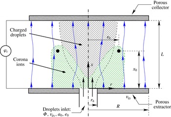
Definition sketch.

2 Formulation
Consider two parallel, porous, metallic disks of radius
 $R$
spaced a distance
 $L$
and kept at constant electric potentials. A gas is injected through one of the disks (the extractor) with uniform velocity
 $v_{g_{I}}$
and sucked through the other (the collector) with the same velocity. An electrospray source generates
 ${\it\Phi}$
droplets of radius
 $a_{0}$
and electric charge
 $-e_{0}$
per unit time, which are injected with velocity
 $v_{p_{I}}$
through an orifice of radius
 $r_{h}$
at the centre of the extractor disk. To neutralize these electrospray droplets before they reach the collector, a corona emitting a current
 $I_{i}$
of ions of the polarity opposite to that of the droplets is generated by a metallic ring of radius
 $r_{0}$
concentric with the inlet orifice, located at a distance
 $x_{0}$
from the extractor and kept at a high voltage relative to it (see figure 1). In what follows the charge of the droplets is conventionally taken to be negative and the charge of the ions positive.
The mean distance between droplets,
 $\ell _{d}$
, is assumed to be large compared with the radius of a droplet and small compared with the size of the spray; i.e.
 $a_{0}\ll \ell _{d}\ll L$
. In these conditions, an Eulerian mesoscale description of the gas flow (Williams Reference Williams1985) combined with a Lagrangian particle-in-cell description of the droplets (Hockney & Eastwood Reference Hockney and Eastwood1988; Birdsall & Langdon Reference Birdsall and Langdon1991) can be used.
2.1 Droplets
The droplets interact mainly through the surrounding gas and through the electric field induced by the electric charges they carry and the voltages applied between the electrodes (disks and wire ring). Direct interactions between droplets are rare events when
 $a_{0}\ll \ell _{d}$
. The electric charge of a droplet changes in time due to the attachment of ions generated by the corona discharge.
Let
 $-e_{j}(t)$
be the electric charge of droplet
 $j$
, and
 $\boldsymbol{x}_{j}(t)$
and
 $\boldsymbol{v}_{j}(t)$
be the position and velocity of its centre. Droplet evaporation and coagulation are not considered. The droplet’s radius
 $a_{0}$
and mass
 $m_{0}={\textstyle \frac{4}{3}}{\rm\pi}{\it\rho}_{l}a_{0}^{3}$
, where
 ${\it\rho}_{l}$
is the density of the liquid, are constant and taken to be the same for all the droplets of the spray, though this condition can be easily released. The momentum and charge conservation equations for droplet
 $j$
are
 $$\begin{eqnarray}\frac{\text{d}\boldsymbol{x}_{j}}{\text{d}t}=\boldsymbol{v}_{j},\quad m_{0}\frac{\text{d}\boldsymbol{v}_{j}}{\text{d}t}=\boldsymbol{F}_{j}-e_{j}\boldsymbol{E}_{j},\quad \frac{\text{d}e_{j}}{\text{d}t}=-{\it\nu}_{j},\end{eqnarray}$$
where
 $\boldsymbol{F}_{j}$
is the force of the gas on the droplet,
 $\boldsymbol{E}_{j}$
is the electric field at the position of the droplet, and
 ${\it\nu}_{j}$
is the rate at which the droplet attaches positive charge from the corona-generated ions. Taking into account the small gas-to-liquid density ratio, the approximation
 $$\begin{eqnarray}\boldsymbol{F}_{j}=-6{\rm\pi}{\it\mu}_{g}a_{0}(\boldsymbol{v}_{j}-\boldsymbol{v}_{g_{j}})\end{eqnarray}$$
can be used for small and moderate values of the Reynolds number of the slip flow,
 $Re_{d_{j}}={\it\rho}_{g}|\boldsymbol{v}_{j}-\boldsymbol{v}_{g_{j}}|a_{0}/{\it\mu}_{g}$
, where
 ${\it\rho}_{g}$
and
 ${\it\mu}_{g}$
are the density and viscosity of the gas, and
 $\boldsymbol{v}_{g_{i}}$
is the velocity of the gas seen by the droplet (see e.g. Sánchez, Urzay & Liñán Reference Sánchez, Urzay and Liñán2015).
Field charging is the dominant mode of ion attachment for electrospray droplets of tens of micrometres immersed in a strong electric field and exposed to corona-generated ions (see e.g. Friedlander Reference Friedlander2000). Assuming that the electric conductivity of the liquid is sufficiently high to keep the surface of droplet
 $j$
approximately equipotential, the field normal to the surface is
 $E_{n}=3|\boldsymbol{E}_{j}|\cos {\it\theta}-e_{j}/4{\rm\pi}{\it\epsilon}_{0}a_{0}^{2}$
, where
 ${\it\theta}$
is the polar angle at the surface of the droplet, with
 ${\it\theta}=0$
in the direction of
 $\boldsymbol{E}_{j}$
, and
 ${\it\epsilon}_{0}$
is the electric permittivity of the gas. Positive ions drift along the lines of field and collide with the region
 ${\it\Sigma}_{-}$
of the droplet surface where
 $E_{n}<0$
. The flux of electric charge reaching the droplet per unit time is
 ${\it\nu}_{j}={\it\kappa}{\it\rho}_{i}\int _{{\it\Sigma}_{-}}(-E_{n})\,\text{d}{\it\sigma}$
, where
 ${\it\kappa}$
is the mobility of the ions and
 ${\it\rho}_{i}$
is the density of charge due to the ions around the droplet. A simple computation gives (White Reference White1963)
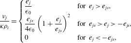 $$\begin{eqnarray}\frac{{\it\nu}_{j}}{{\it\kappa}{\it\rho}_{i}}=\left\{\begin{array}{@{}ll@{}}\displaystyle \frac{e_{j}}{{\it\epsilon}_{0}}\quad & \text{for }e_{j}>e_{js},\\ \displaystyle \frac{e_{js}}{4{\it\epsilon}_{0}}\left(1+\frac{e_{j}}{e_{js}}\right)^{2}\quad & \text{for }e_{js}>e_{j}>-e_{js},\\ \displaystyle 0\quad & \text{for }e_{j}<-e_{js},\end{array}\right.\end{eqnarray}$$
with
 $e_{js}=12{\rm\pi}{\it\epsilon}_{0}|\boldsymbol{E}_{j}|a_{0}^{2}$
, which is the maximum (saturation) positive charge that droplet
 $j$
can attain by field charging under the action of a field
 $|\boldsymbol{E}_{j}|$
.
Droplets are continuously injected through the inlet orifice of radius
 $r_{h}$
with initial conditions
 $$\begin{eqnarray}x_{j}=0,\quad r_{j}=\text{rand}[f(r)],\quad \boldsymbol{v}_{j}=v_{p_{I}}\boldsymbol{i},\quad e_{j}=e_{0}\quad \text{at }t=j/{\it\Phi},\end{eqnarray}$$
and they evolve according to (2.1) until they hit one of the disks or reach the periphery of the disks. Here
 $x$
and
 $r$
are distances along and normal to the axis of the orifice, with
 $x=0$
at the orifice,
 $\boldsymbol{i}$
is a unit axial vector,
 ${\it\Phi}$
is the number of droplets injected per unit time, and
 $$\begin{eqnarray}f(r)=\frac{1-\exp (-r^{2}/r_{c}^{2})}{1-\exp (-r_{h}^{2}/r_{c}^{2})}\quad \text{for }r<r_{h},\quad f(r)=1\quad \text{for }r>r_{h}\end{eqnarray}$$
is the cumulative distribution of initial droplet positions, which is an axisymmetric Gaussian with standard deviation
 $r_{c}<r_{h}$
truncated at the orifice radius. Conditions (2.4) are for a liquid flow rate
 $Q={\textstyle \frac{4}{3}}{\rm\pi}a_{0}^{3}{\it\Phi}$
injected as a monodisperse spray that carries an electric current
 $I_{d}=-e_{0}{\it\Phi}$
. They can be easily generalized to account for sprays made of various classes of droplets, with different radii and initial charges and velocities.
Since the number of droplets present between the disks may be very large, a method of particles (Hockney & Eastwood Reference Hockney and Eastwood1988; Birdsall & Langdon Reference Birdsall and Langdon1991) is used in which each particle represents a parcel of the one-droplet phase space containing a constant number of identical droplets. Each particle has the same radius and mass as the droplets it represents, and obeys the same equations (2.1)–(2.3). However, when it comes to evaluating the contribution of a particle to the space charge (which is
 $e_{j}$
for a droplet), or to the force exerted on the gas (the opposite of
 $\boldsymbol{F}_{j}$
in (2.2) for a droplet), or to the rate at which ions are attached (
 ${\it\nu}_{j}$
in (2.3) for a droplet), each particle counts for as many droplets as it represents. Particles are continuously injected with the initial conditions (2.4) of the represented droplets, but the number of particles injected per unit time is the number of droplets,
 ${\it\Phi}$
, divided by the number of droplets per particle. This number is a free parameter of the method, and there may be many fewer particles in the simulation than there are droplets in the real spray. The numerical burden is reduced by decreasing the number of equations (2.1) that must be simultaneously solved. Axisymmetry is imposed with the method of particles by assuming that a particle injected at a certain distance
 $r$
from the centre of the inlet orifice amounts to
 $2{\rm\pi}{\it\xi}$
identical droplets equispaced on a circumference of radius
 $r$
(Birdsall & Langdon Reference Birdsall and Langdon1991). The time between particle injections is then
 $2{\rm\pi}{\it\xi}/{\it\Phi}$
, which replaces
 $1/{\it\Phi}$
in (2.4); see (Higuera Reference Higuera2016) for details of the implementation.
2.2 Electric potential and corona
A corona is assumed to be generated by a wire of radius
 $b_{w}$
raised to a high voltage relative to the extractor disk. The wire is shaped as a ring of radius
 $r_{0}$
concentric with the inlet orifice at a distance
 $x_{0}$
above it (see figure 1). In what follows
 $b_{w}\ll r_{0}$
is assumed. No attempt is made to simulate the wire and the small region of high electric field around the wire where ionization of the gas occurs. Instead, the wire is modelled as a line of charge and the ionic current issuing from the high-field region is represented by a source of positive charge distributed around this line. The strength of the source is the corona current, which is a parameter of the model. The electric potential at a distance
 $b_{w}$
from the line plays in the model the role of the voltage of the wire. It is computed as part of the solution.
The equations governing the electric potential and the density of ionic charge are discussed in turn in this section.
The electric potential
 ${\it\varphi}$
, with
 $\boldsymbol{E}=-\boldsymbol{{\rm\nabla}}{\it\varphi}$
, satisfies the Poisson equation
 $$\begin{eqnarray}{\rm\nabla}^{2}{\it\varphi}=-\frac{1}{{\it\epsilon}_{0}}[{\it\rho}_{i}-{\it\rho}_{d}+q_{w}{\it\delta}(x-x_{0}){\it\delta}(r-r_{0})],\end{eqnarray}$$
with the conditions
 ${\it\varphi}=0$
at the extractor (
 $x=0$
) and
 ${\it\varphi}={\it\varphi}_{c}$
at the collector (
 $x=L$
). Here
 ${\it\rho}_{i}$
is the density of positive space charge due to the corona ions;
 ${\it\rho}_{d}$
is the density of negative space charge due to the droplets, given by (2.13) below;
 $q_{w}$
is the charge per unit length of the line modelling the ring;
 ${\it\delta}$
is the Dirac delta function; and
 ${\it\varphi}_{c}$
is the potential of the collector.
It may be noted for future reference that the electric potential of a circular line of charge isolated in unbounded space is (see e.g. Landau & Lifshitz Reference Landau and Lifshitz1960)
 $$\begin{eqnarray}{\it\varphi}_{l}(x,r)=\frac{q_{w}}{{\it\epsilon}_{0}}G(x,r;x_{0},r_{0}),\end{eqnarray}$$
with
 $$\begin{eqnarray}G(x,r;x_{0},r_{0})=\frac{1}{{\rm\pi}}\frac{r_{0}K(m)}{[(x-x_{0})^{2}+(r+r_{0})^{2}]^{1/2}}\quad \text{and}\quad m=\frac{4rr_{0}}{(x-x_{0})^{2}+(r+r_{0})^{2}},\end{eqnarray}$$
where
 $K(m)$
is the complete elliptic integral of the first kind. The electric potential and field at a distance
 $b_{w}\ll r_{0}$
from the line are
 ${\it\varphi}_{lw}\approx -q_{w}/(2{\rm\pi}{\it\epsilon}_{0})\ln (b_{w}/8r_{0})$
and
 $E_{w}\approx q_{w}/(2{\rm\pi}{\it\epsilon}_{0}b_{w})$
, pointing away from the line. The potential of the collector is set to
 ${\it\varphi}_{c}={\it\varphi}_{l}(x=L,r=0)$
, which is proportional to
 $q_{w}$
, in what follows.
This result is useful to solve (2.6) in the space between the extractor and the collector because the function
 ${\it\varphi}_{l}$
contains the singular part of the solution, which can be easily separated. Consider first the electric potential
 ${\it\varphi}_{h}$
due to the line of charge only, with
 ${\it\rho}_{i}$
and
 ${\it\rho}_{d}$
omitted from (2.6). The potential
 ${\it\varphi}_{h}$
is singular at (
 $x_{0},r_{0}$
) but the difference
 ${\it\varphi}_{h}^{\prime }={\it\varphi}_{h}-{\it\varphi}_{l}$
is finite and has a finite gradient at this point; it satisfies Laplace’s equation and is equal to
 $-{\it\varphi}_{l}$
at the extractor and to
 ${\it\varphi}_{c}-{\it\varphi}_{l}$
at the collector. The electric potential at a distance
 $b_{w}\ll r_{0}$
from the line of charge (the voltage of the wire in the approximation of the model) is
 ${\it\varphi}_{hw}\approx {\it\varphi}_{lw}+{\it\varphi}_{h}^{\prime }(x_{0},r_{0})$
in the absence of space charge.
When corona ions and charged droplets are present in the space between the disks, the electric potential can be written in the form
 ${\it\varphi}={\it\varphi}_{h}+{\it\varphi}_{sc}$
, where
 ${\it\varphi}_{sc}$
, the contribution of the space charge, satisfies
 $$\begin{eqnarray}{\rm\nabla}^{2}{\it\varphi}_{sc}=\frac{{\it\rho}_{d}-{\it\rho}_{i}}{{\it\epsilon}_{0}},\end{eqnarray}$$
with
 ${\it\varphi}_{sc}=0$
at the extractor and collector. In particular, the value of
 ${\it\varphi}_{sc}$
at (
 $x_{0},r_{0}$
) is the variation of the wire voltage due to the space charge. The electric field at a distance
 $b_{w}\ll r_{0}$
from the line of charge is still approximately equal to
 $E_{w}$
above.
A corona first appears on the wire ring when the electric field at its surface reaches a certain threshold value that depends on the radius of the wire and the properties of the gas (Raizer Reference Raizer1997). This electric field stays nearly constant at its threshold value when the ionic current
 $I_{i}$
generated by the corona is increased by increasing the voltage of the wire (see e.g. Raizer Reference Raizer1997). In what follows
 $E_{w}$
is understood as the corona threshold field at the surface of the wire, unless otherwise noted. The relation
 $q_{w}=2{\rm\pi}{\it\epsilon}_{0}b_{w}E_{w}$
then determines the strength of the equivalent line of charge required to achieve a corona discharge for a wire of given radius, and
 ${\it\varphi}_{hw}$
is the threshold voltage of the wire in the absence of droplets. The condition that
 $E_{w}$
stays nearly constant at its threshold value when the corona is established is satisfied by keeping
 $q_{w}$
constant, independent of the corona current.
The ionization process leading to the corona current is not analysed here. As was mentioned before, ion generation is modelled by means of a source of positive charge distributed around the line of charge. The source distribution is arbitrarily taken to be a Gaussian,
 $$\begin{eqnarray}S_{i}=\frac{I_{i}}{2{\rm\pi}^{2}r_{0}b_{i}}\exp \left[-\frac{(x-x_{0})^{2}+(r-r_{0})^{2}}{b_{i}^{2}}\right]\quad \text{with }b_{i}\ll r_{0},\end{eqnarray}$$
where
 $I_{i}$
is the total ionic current
 $(I_{i}=\int \!2{\rm\pi}rS_{i}\,\text{d}x\,\text{d}r)$
and
 $b_{i}$
is the standard deviation of the Gaussian.
The ionic charge is convected by the gas flow, drifts relative to the gas due to the mobility of the ions, and disappears when the ions are attached to electrospray droplets or reach the disks. The charge density of corona ions satisfies the conservation equation
 $$\begin{eqnarray}\frac{\partial {\it\rho}_{i}}{\partial t}+\boldsymbol{{\rm\nabla}}\boldsymbol{\cdot }[{\it\rho}_{i}(\boldsymbol{v}_{g}+{\it\kappa}\boldsymbol{E})]=S_{i}-{\it\nu},\end{eqnarray}$$
where
 ${\it\nu}$
is the rate at which ions are attached by the droplets per unit volume and time, which is given by (2.13) below.
It may be noted at this point that the parameters
 $E_{w}$
and
 $b_{w}$
appear only through the combination
 $q_{w}=2{\rm\pi}{\it\epsilon}_{0}b_{w}E_{w}$
in the line-of-charge model of the wire. The radius of the wire does not explicitly appear in the formulation of the electric problem if
 $q_{w}$
is used as a control parameter; it reappears only when the contribution
 ${\it\varphi}_{lw}$
to the voltage of the wire is evaluated at the end of the computation. The extent to which this simple model reproduces the features of a real corona is discussed in § 3.1 below.
An alternative to the volumetric source representation (2.10) would be to assume that the ions come from the wire surface. This, however, would bring
 $b_{w}$
back into the problem and make for stiff numerical problems, as a fine grid fitted to the thin wire would be required.
Collisions of the droplets with the corona wire are not taken into account. The high mobility of the corona ions is expected to prevent charged droplets from massively reaching the wire when neutralization is efficient and the distance from the wire to the spray is properly chosen. Charged droplets may reach the wire when it is charged to a high voltage but no corona exists (as in § 3.2 below), or when the corona current is small and the wire is within the spray plume. These, however, are not suitable conditions for neutralization. Collisions of neutralized droplets with the wire are rare for a dilute spray.
2.3 Gas
Conservation equations for the mesoscale description of the gas (Williams Reference Williams1985) can be derived from the principles of conservation of mass and momentum applied to the gas in elementary volumes of size large compared to
 $\ell _{d}$
but small compared to
 $L$
. These volumes enclose many droplets that exchange momentum with the gas, whose effect appears as a distributed force in the momentum equation. Fluctuations of the gas velocity and pressure about their local average values are small everywhere except in the vicinity of each droplet, and can be left out (Sánchez et al.
Reference Sánchez, Urzay and Liñán2015). The volume fraction of droplets is also negligible. In the absence of thermal and compressibility effects, the continuity and momentum equations for the gas phase are
 $$\begin{eqnarray}\boldsymbol{{\rm\nabla}}\boldsymbol{\cdot }\boldsymbol{v}_{g}=0,\quad {\it\rho}_{g}\left(\frac{\partial \boldsymbol{v}_{g}}{\partial t}+\boldsymbol{v}_{g}\boldsymbol{\cdot }\boldsymbol{{\rm\nabla}}\boldsymbol{v}_{g}\right)=-\boldsymbol{{\rm\nabla}}p_{g}+{\it\mu}_{g}{\rm\nabla}^{2}\boldsymbol{v}_{g}-\boldsymbol{F}+{\it\rho}_{i}\boldsymbol{E},\end{eqnarray}$$
where
 $\boldsymbol{v}_{g}$
and
 $p_{g}$
are the mesoscale-averaged gas velocity and pressure, and the last two terms on the right-hand side of the momentum equation are the forces of the droplets and the ions on the unit volume of gas, with
 $\boldsymbol{F}$
given by (2.13) below.
Axisymmetric solutions of these equations are sought subjected to the boundary conditions
 $\boldsymbol{v}_{g}=v_{g_{I}}\boldsymbol{i}$
at the extractor and collector surfaces,
 $x=0$
and
 $L$
, and approximate inlet/outlet conditions at the open periphery of these electrode disks (see (2.23) below). The effect of the wire electrode on the motion of the gas is neglected. As with individual droplets, the wire causes only a small perturbation to the gas flow, except at distances from the wire of the order of its radius. The force of the wire on the gas is small compared to the force of the spray on the gas.
The source terms in (2.9), (2.11) and (2.12) are (Sánchez et al. Reference Sánchez, Urzay and Liñán2015; Higuera Reference Higuera2016)
 $$\begin{eqnarray}{\it\nu}=2{\rm\pi}{\it\xi}\frac{\sum {\it\nu}_{j}}{{\it\delta}{\it\Omega}},\quad {\it\rho}_{d}=2{\rm\pi}{\it\xi}\frac{\sum e_{j}}{{\it\delta}{\it\Omega}},\quad \boldsymbol{F}=2{\rm\pi}{\it\xi}\frac{\sum \boldsymbol{F}_{j}}{{\it\delta}{\it\Omega}},\end{eqnarray}$$
where the sums are over the particles present in a toroidal control volume
 ${\it\delta}{\it\Omega}$
of cross-section centred at point
 $\boldsymbol{x}$
at time
 $t$
, and the formal limit
 ${\it\delta}{\it\Omega}\rightarrow 0$
is understood (see Williams (Reference Williams1985) for a definition in terms of the moments of the droplet distribution function).
For the numerical treatment, equations (2.12) are rewritten in the equivalent stream- function–vorticity form. They are discretized along with (2.11) and (2.9) using finite differences, and marched in time together with (2.1) using second-order methods. A Crank–Nicolson method with a standard preconditioned biconjugate gradient is used for the viscous term of the vorticity equation and an Adams–Bashforth method is used for the rest. A non-uniform
 $240\times 240$
grid, finer around the symmetry axis and the injection orifice, and a dimensionless time step of
 $2\times 10^{-3}$
are used. The toroidal volumes generated by rotating grid cells around the symmetry axis are used for
 ${\it\delta}{\it\Omega}$
.
2.4 Dimensionless variables
In what follows, distances are scaled with the distance
 $L$
between the disks, times with the stopping time
 $t_{0}=m_{0}/c_{f}$
, where
 $m_{0}={\textstyle \frac{4}{3}}{\rm\pi}{\it\rho}_{l}a_{0}^{3}$
and
 $c_{f}=6{\rm\pi}{\it\mu}_{g}a_{0}$
, velocities with
 $v_{0}=L/t_{0}$
, droplet radius and charge with
 $a_{0}$
and
 $e_{0}$
, and the electric field and electric potential with
 $E_{0}$
and
 $E_{0}L$
, where
 $E_{0}=n_{0}e_{0}L/{\it\epsilon}_{0}$
and
 $n_{0}={\it\Phi}/v_{0}L^{2}$
. The charge densities due to the droplets and the ions are both scaled with
 $e_{0}n_{0}$
, the ionic current
 $I_{i}$
with
 $-I_{d}=e_{0}{\it\Phi}$
, the ion’s mobility
 ${\it\kappa}$
with
 $v_{0}/E_{0}$
, and
 $q_{w}$
with
 $e_{0}n_{0}L^{2}$
.
Denoting the dimensionless variables with the same symbols as used before for their dimensional counterparts, the governing equations take the form
 $$\begin{eqnarray}\frac{\text{d}\boldsymbol{x}_{j}}{\text{d}t}=\boldsymbol{v}_{j},\quad \frac{\text{d}\boldsymbol{v}_{j}}{\text{d}t}=\boldsymbol{F}_{j}-{\it\Pi}e_{j}\boldsymbol{E}_{j},\quad \frac{\text{d}e_{j}}{\text{d}t}=-{\it\nu}_{j},\end{eqnarray}$$
with
 $$\begin{eqnarray}\boldsymbol{F}_{j}=-(\boldsymbol{v}_{j}-\boldsymbol{v}_{g_{j}})\quad \text{and}\quad {\it\nu}_{j}={\it\rho}_{i}{\it\kappa}\left\{\begin{array}{@{}ll@{}}e_{j}\quad & \text{for }e_{j}>e_{js},\\ \displaystyle \frac{e_{js}}{4}\left(1+\frac{e_{j}}{e_{js}}\right)^{2}\quad & \text{for }e_{js}>e_{j}>-e_{js},\\ 0\quad & \text{for }e_{j}<-e_{js},\end{array}\right.\end{eqnarray}$$
with
 $e_{js}=e_{s}|\boldsymbol{E}_{j}|$
. Here, as before,
 $\boldsymbol{E}_{j}$
and
 $\boldsymbol{v}_{g_{j}}$
are the electric field and the gas velocity interpolated to the position
 $\boldsymbol{x}_{j}$
of particle
 $j$
at time
 $t$
. These equations are to be solved with the injection conditions
 $$\begin{eqnarray}x_{j}=0,\quad r_{j}=\text{rand}[f(r)],\quad \boldsymbol{v}_{j}=v_{p_{I}}\boldsymbol{i},\quad e_{j}=1\quad \text{at }t=j{\it\eta},\end{eqnarray}$$
with
 $f(r)$
given by (2.5),
 $$\begin{eqnarray}\boldsymbol{{\rm\nabla}}\boldsymbol{\cdot }\boldsymbol{v}_{g}=0,\quad \frac{\partial \boldsymbol{v}_{g}}{\partial t}+\boldsymbol{v}_{g}\boldsymbol{\cdot }\boldsymbol{{\rm\nabla}}\boldsymbol{v}_{g}=-\boldsymbol{{\rm\nabla}}p_{g}+\frac{1}{Re}{\rm\nabla}^{2}\boldsymbol{v}_{g}-\mathscr{F}\boldsymbol{F}+{\it\Pi}\mathscr{F}{\it\rho}_{i}\boldsymbol{E},\end{eqnarray}$$
 $$\begin{eqnarray}\displaystyle & \displaystyle \frac{\partial {\it\rho}_{i}}{\partial t}+\boldsymbol{{\rm\nabla}}\boldsymbol{\cdot }[{\it\rho}_{i}(\boldsymbol{v}_{g}+{\it\kappa}\boldsymbol{E})]=S_{i}-{\it\nu}, & \displaystyle\end{eqnarray}$$
 $$\begin{eqnarray}\displaystyle & \displaystyle {\rm\nabla}^{2}{\it\varphi}={\it\rho}_{d}-{\it\rho}_{i}-q_{w}{\it\delta}(x-x_{0}){\it\delta}(r-r_{0}), & \displaystyle\end{eqnarray}$$
with
 $S_{i}$
given by (2.10),
 $\boldsymbol{E}=-\boldsymbol{{\rm\nabla}}{\it\varphi}$
,
 $$\begin{eqnarray}{\it\nu}={\it\eta}\frac{\sum {\it\nu}_{j}}{{\it\delta}{\it\Omega}},\quad {\it\rho}_{d}={\it\eta}\frac{\sum e_{j}}{{\it\delta}{\it\Omega}},\quad \boldsymbol{F}={\it\eta}\frac{\sum \boldsymbol{F}_{j}}{{\it\delta}{\it\Omega}},\end{eqnarray}$$
and the boundary conditions
 $$\begin{eqnarray}\boldsymbol{v}_{g}=v_{g_{I}}\boldsymbol{i},\quad {\it\varphi}=0\quad \text{at }x=0,\end{eqnarray}$$
 $$\begin{eqnarray}\boldsymbol{v}_{g}=v_{g_{I}}\boldsymbol{i},\quad {\it\varphi}={\it\varphi}_{c}\quad \text{at }x=1,\end{eqnarray}$$
 $$\begin{eqnarray}\left.\begin{array}{@{}c@{}}\displaystyle u_{g}=0,\quad {\bf\omega}_{g}=0\quad \text{if }v_{g}<0\quad \text{and}\quad \frac{\partial {\bf\omega}_{g}}{\partial r}=0\quad \text{if }v_{g}>0\\ \displaystyle \frac{\partial (rE_{r})}{\partial r}=0\end{array}\right\}\quad \text{at }r=R,\end{eqnarray}$$
where
 ${\it\varphi}_{c}=q_{w}G(1,0;x_{0},r_{0})$
with
 $G$
given by (2.8),
 $u_{g}$
and
 $v_{g}$
are the axial and radial components of the gas velocity, and
 ${\bf\omega}_{g}=\boldsymbol{{\rm\nabla}}\times \boldsymbol{v}_{g}$
is the vorticity. Equation (2.18) needs a boundary condition (
 ${\it\rho}_{i}=0$
) only at regions of the boundary where
 $\boldsymbol{v}_{g}+{\it\kappa}\boldsymbol{E}$
points inwards. The decomposition of the electric potential discussed in § 2.2 into regular and singular parts is used to solve (2.19). The Poisson equation for the full potential is written for definiteness.
The problem contains the 15 dimensionless parameters
 $$\begin{eqnarray}\left.\begin{array}{@{}c@{}}\displaystyle {\it\Pi}=\frac{m_{0}^{2}e_{0}^{2}{\it\Phi}}{{\it\epsilon}_{0}c_{f}^{3}L^{3}},\quad Re=\frac{{\it\rho}_{g}c_{f}L^{2}}{m_{0}{\it\mu}_{g}},\quad \mathscr{F}=\frac{m_{0}^{2}{\it\Phi}}{{\it\rho}_{g}c_{f}L^{3}},\\ \displaystyle q_{w},\;I_{i},\;{\it\kappa},\;e_{s}=12{\rm\pi}\frac{m_{0}a_{0}^{2}{\it\Phi}}{c_{f}L^{2}},\;v_{p_{I}},\;v_{g_{I}},\;x_{0},\;r_{0},\;R,\;r_{h},\;r_{c},\;b_{i},\end{array}\right\}\end{eqnarray}$$
plus the numerical parameter
 ${\it\eta}=2{\rm\pi}c_{f}{\it\xi}/m_{0}{\it\Phi}$
, which measures the number of droplets per particle of the particle method scaled with
 $n_{0}L^{3}$
. In the numerical simulations, the value of this parameter is chosen for the mean number of particles between extractor and collector to be of the order of
 $10^{4}$
, which occurs for
 ${\it\eta}=4\times 10^{-2}$
with the typical spray conditions described in the following section. The number of droplets per particle is then
 ${\it\xi}=O(1)$
. The mean numbers of particles in the volumes
 ${\it\delta}{\it\Omega}$
based on the grid cells are small, especially around the symmetry axis and the boundary of the spray, leading to large fluctuations of the instantaneous values of the source terms (2.20). Numerical tests have been done in which the number of particles is increased, and the fluctuations correspondingly decreased, by reducing
 ${\it\eta}$
by a factor of up to 100. In these conditions, which are not normally used, each particle is a parcel of the droplet phase space that contains less than one droplet, and the number of particles being tracked is larger than the number of droplets. The tests show that the change in the level of the fluctuations has no important effect on the gas and electric variables, nor on the particle variables averaged over a large number of time steps.
Parameter
 $v_{p_{I}}$
is a measure of the stopping distance of the droplets, scaled with
 $L$
, in the absence of gas flow and electric forces. In addition, if the ratio of
 $L$
to the injection velocity of the gas is used as a time scale of the flow,
 $v_{g_{I}}$
in (2.24) is a Stokes number,
 $v_{g_{I}}Re$
is a characteristic Reynolds number, and
 $\mathscr{F}/v_{g_{I}}$
is a characteristic mass loading (mass of liquid per unit mass of gas). These, however, are not the only possible scales. The balance of drag and electric force in the second of equations (2.14) leads to the characteristic dimensionless droplet velocity
 $v_{de}=q_{w}{\it\Pi}$
(using
 $q_{w}$
as a characteristic dimensionless electric field, from (2.19)), while the balance of gas inertia and apparent body force due to the droplets in the second of equations (2.17) leads to the characteristic dimensionless gas velocity
 $v_{ge}=\mathscr{F}^{1/2}$
. With these scales,
 $\mathscr{F}^{1/2}$
is a characteristic Stokes number,
 $\mathscr{F}^{1/2}Re$
is a characteristic Reynolds number, and
 $\mathscr{F}/q_{w}{\it\Pi}$
is a characteristic mass loading. The multiscale character of the problem points to different responses in different regions of the parameter space, and to solution structures featuring multiple regions.
3 Results and discussion
No attempt is made here to explore the large parameter space of the problem. Instead, a single set of electrospray and geometrical conditions is considered and the parameters
 $q_{w}$
and
 $I_{i}$
, which characterize the corona discharge, are varied.
The inlet conditions of the electrospray droplets are taken from an experiment reported by Deng & Gomez (Reference Deng and Gomez2007) in which a flow rate
 $Q=0.6~\text{ml}~\text{h}^{-1}$
of ethanol (
 ${\it\rho}_{l}=790~\text{kg}~\text{m}^{-3}$
) carrying an electric current
 $I_{d}=-24.5~\text{nA}$
(determined from scaling laws) is electrosprayed into droplets of diameter
 $2a_{0}=11~{\rm\mu}\text{m}$
. This amounts to
 $m_{0}=5.5\times 10^{-13}~\text{kg}$
,
 ${\it\Phi}=Q/({\textstyle \frac{4}{3}}{\rm\pi}a_{0}^{3})=2.39\times 10^{5}~\text{s}^{-1}$
and
 $e_{0}=-I_{d}/{\it\Phi}=1.025\times 10^{-13}~\text{C}$
, for which (in air, with
 ${\it\rho}_{g}=1.225~\text{kg}~\text{m}^{-3}$
and
 ${\it\mu}_{g}=1.78\times 10^{-5}~\text{kg}~\text{m}^{-1}~\text{s}^{-1}$
)
 $c_{f}=1.845\times 10^{-9}~\text{kg}~\text{s}^{-1}$
,
 $v_{0}=33.49~\text{m}~\text{s}^{-1}$
,
 $n_{0}=7.136\times 10^{7}~\text{m}^{-3}$
and
 $E_{0}=8.261\times 10^{3}~\text{V}~\text{m}^{-1}$
. The droplets are injected with a velocity of
 $8.37~\text{m}~\text{s}^{-1}$
through an orifice of diameter 0.228 mm at the centre of the extractor disk. The extractor-to-collector distance is
 $L=10~\text{mm}$
, equal to the radius of both disks. The radius of the ring generating the corona (not present in the experiment of Deng & Gomez (Reference Deng and Gomez2007)) is taken to be 5 mm, and it is located half-way between the two disks. The mobility of the corona ions is
 $2.2\times 10^{-4}~\text{m}^{2}~\text{V}^{-1}~\text{s}^{-1}$
(Zhao & Adamiak Reference Zhao and Adamiak2005), and the inlet velocity of the air is
 $0.33~\text{m}~\text{s}^{-1}$
. In these conditions,
 $$\begin{eqnarray}\left.\begin{array}{@{}c@{}}{\it\Pi}=1.37\times 10^{-2},\quad Re=2.31\times 10^{5},\quad \mathscr{F}=3.21\times 10^{-5},\\ {\it\kappa}=5.43\times 10^{-2},\quad e_{s}=8.14\times 10^{-4},\quad v_{p_{I}}=0.25,\quad v_{g_{I}}=10^{-2},\\ x_{0}=r_{0}=0.5,\quad R=1,\quad r_{h}=1.14\times 10^{-2},\quad r_{c}=5.7\times 10^{-3},\quad b_{i}=2\times 10^{-2}.\end{array}\right\}\end{eqnarray}$$
Parameter
 $e_{s}$
is a measure of the ratio of the saturation charge of a droplet under a dimensionless electric field of order unity to (minus) the initial charge of the droplet. Its small value means that the initial charge of the droplet is large compared to the charge that an initially neutral droplet may acquire by field charging. The dimensionless voltage of the collector is
 ${\it\varphi}_{c}={\it\varphi}_{l}(x=1,r=0)=0.707q_{w}$
in these conditions.
The estimated number of droplets between extractor and collector is smaller in the experiment of Deng & Gomez (Reference Deng and Gomez2007) than in the numerical simulations discussed below by a factor of approximately 40. This is probably due to the absence of neutralization and to the strong driving electric field (due to the voltage
 ${\it\varphi}_{c}$
applied between collector and extractor) used in the experiment. The estimated mean distance between droplets is of the order of 0.5 mm far from the injection orifice, both in the experiment and in the simulations, but in the experiment the spray of a single source occupies only a small fraction of the space between the disks.
3.1 Corona without spray
Some computations without droplets (
 ${\it\eta}=0$
in (2.20)) have been carried out to check the corona model introduced in § 2.2. The properties of the droplets disappear from the formulation by using the rescaled variables
 $\widetilde{{\it\rho}}_{i}={\it\rho}_{i}/q_{w}$
,
 $\widetilde{{\it\varphi}}={\it\varphi}/q_{w}$
and
 $\widetilde{\boldsymbol{v}}=\boldsymbol{v}/[({\it\Pi}\mathscr{F})^{1/2}q_{w}]$
. The solution of the reduced problem depends only on the parameters
 $\widetilde{I}_{i}=I_{i}/[({\it\Pi}\mathscr{F})^{1/2}q_{w}^{2}]$
,
 $\widetilde{Re}=({\it\Pi}\mathscr{F})^{1/2}q_{w}Re$
,
 $\widetilde{v}_{g_{I}}=v_{g_{I}}/[({\it\Pi}\mathscr{F})^{1/2}q_{w}]$
,
 $\widetilde{{\it\kappa}}={\it\kappa}/({\it\Pi}\mathscr{F})^{1/2}$
,
 $x_{0}$
,
 $r_{0}$
,
 $R$
and
 $b_{i}$
.
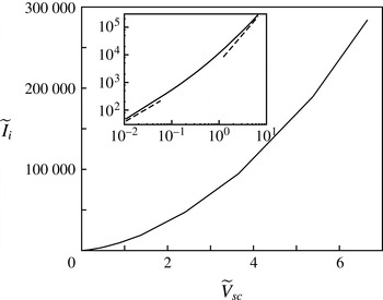
Figure 2 shows the computed current–voltage characteristic of the corona in the absence of gas injection (
 $\widetilde{v}_{g_{I}}=0$
). Here
 $\widetilde{V}_{sc}=\widetilde{{\it\varphi}}-\widetilde{{\it\varphi}}_{h}$
at (
 $x_{0},r_{0}$
) is the rescaled ring voltage referred to the corona threshold voltage (the dimensionless form of
 ${\it\varphi}_{hw}$
of § 2.2), while the rescaled threshold electric field at the surface of the wire is
 $\widetilde{E}_{w}=1/(2{\rm\pi}b_{w})$
within the approximation of the model. The results (see logarithmic inset) show the well-known transition from a linear characteristic near the threshold voltage towards a quadratic one for large values of the voltage, when the effect of the space charge matters and eventually dominates the electric potential (Raizer Reference Raizer1997).
Current–voltage characteristic of the corona without droplets for
 $\widetilde{Re}=153.19$
,
 $\widetilde{v}_{g_{I}}=0$
and
 $\widetilde{{\it\kappa}}=81.88$
. Other parameters have the values given in (3.1). The dashed lines at the left- and right-hand sides of the inset have slopes 1 and 2, respectively.

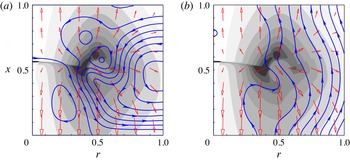
Charge density of ions
 ${\it\rho}_{i}$
(10 grey levels between 0 (white) and 10 (darkest)), streamlines of the gas (solid, with arrows) and electric field (open red arrows) for
 $\widetilde{I}_{i}=753.98$
,
 $\widetilde{Re}=153.19$
,
 $\widetilde{{\it\kappa}}=81.88$
and
 $\widetilde{v}_{g_{I}}=0$
(a) and 0.15 (b).

These results can be rationalized as follows. In dimensional variables, the electric field induced by the line of charge at distances of order
 $L$
from the line is
 $E_{h}\sim q_{w}/{\it\epsilon}_{0}L$
up to a logarithmic factor. The order of the charge density of corona ions drifting in this field is determined by the current conservation condition
 ${\it\rho}_{i}{\it\kappa}E_{h}L^{2}\sim I_{i}$
, while the field induced by this space charge is
 $E_{sc}\sim {\it\rho}_{i}L/{\it\epsilon}_{0}\sim I_{i}/{\it\epsilon}_{0}{\it\kappa}E_{h}L$
, from the Poisson equation
 $\boldsymbol{{\rm\nabla}}\boldsymbol{\cdot }\boldsymbol{E}_{sc}={\it\rho}_{i}/{\it\epsilon}_{0}$
. This field becomes of the order of
 $E_{h}$
when
 $I_{i}\sim I_{ic}={\it\kappa}q_{w}^{2}/{\it\epsilon}_{0}L$
(or
 $\widetilde{I}_{ic}=\widetilde{{\it\kappa}}$
in dimensionless variables). For
 $I_{i}\ll I_{ic}$
, the space-charge-induced field and thus the variation of the ring’s potential about the corona threshold value are proportional to
 $I_{i}$
. For
 $I_{i}\gg I_{ic}$
, the space-charge-induced field dominates in ample regions, where the current conservation condition becomes
 ${\it\rho}_{i}{\it\kappa}E_{sc}L^{2}\sim I_{i}$
, which, together with the Poisson equation balance
 $E_{sc}/L\sim {\it\rho}_{i}/{\it\epsilon}_{0}$
, leads to
 $I_{i}\sim {\it\epsilon}_{0}{\it\kappa}E_{sc}^{2}$
and thus to a corona current that increases quadratically with the ring’s potential.
Figure 3 shows the density of ions (grey levels) for
 $\widetilde{I}_{i}=753.98$
with
 $\widetilde{v}_{g_{I}}=0$
(a) and 0.15 (b). The density is largest around the injection region that models the ionization region surrounding the ring, and the distribution becomes lozenge-shaped where the effects of the radius of the ring and the planar extractor and collector disks come into play. The force of the ions on the gas (last term of (2.17)) induces the so-called ionic wind, whose streamlines are shown in figure 3(a) (solid curves) in the absence of gas injection (
 $\widetilde{v}_{g_{I}}=0$
). Figure 3(b), for
 $\widetilde{v}_{g_{I}}=0.15$
, shows that a weak forced flow suffices to overcome the ionic wind with only small changes of the distribution of ions. As in other instances of corona discharges (Yamamoto & Velkoff Reference Yamamoto and Velkoff1981; Kallio & Stock Reference Kallio and Stock1992), the velocity of the gas is small compared with the drift velocity of the ions,
 $\widetilde{{\it\kappa}}\widetilde{\boldsymbol{E}}$
in (2.18), so that the ions nearly follow the electric field (open red arrows in figure 3). The electric and hydrodynamic problems become uncoupled if
 $\boldsymbol{v}_{g}$
is neglected in (2.18), and the stationary solution of the first of these problems then depends on
 $\widetilde{I}_{i}/\widetilde{{\it\kappa}}$
rather than on these two parameters separately.
The problem formulation of § 2 shows that the evolution of the ions is uncoupled from the rest of the problem when: (i) their drift velocity is large compared to the velocity of the gas; (ii) the electric field on which the drift velocity depends is determined by the potentials applied to the electrodes and the space charge of the ions only; and (iii) the ion sink due to attachment is negligible. The last two conditions are not satisfied when charged droplets are present, unless the electric field induced by the charge of the droplets is small compared to the field induced by the charge of the ions (
 ${\it\rho}_{d}\ll {\it\rho}_{i}$
) or to the applied field, which are not conditions usually met in spray neutralization. The first condition may still hold in the presence of droplets. If the residence time of the ions between the extractor and collector is small compared to those of the gas and the droplets, then the distribution of ions can be assumed to adapt instantly to the conditions of the spray. This approximation, however, is not used in § 3.3 below.
3.2 Spray without corona
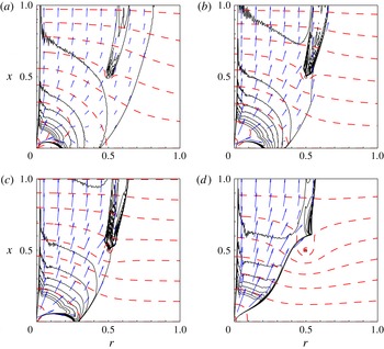
Number density of droplets (
 $n_{d}={\it\eta}\sum 1_{j}/{\it\delta}{\it\Omega}$
, where
 $\sum 1_{j}$
is the number of particles in
 ${\it\delta}{\it\Omega}$
; 10 solid, equispaced contours between 0 and 60, with largest values around the injection orifice), equipotentials of the electric field (dashed) and mean velocity of the droplets (arrows), defined as
 $\langle \boldsymbol{v}_{d}\rangle =n_{d}^{-1}{\it\eta}\sum \boldsymbol{v}_{j}/{\it\delta}{\it\Omega}$
, for
 $I_{i}=0$
and
 $q_{w}=3$
(a), 5 (b), 7 (c) and 10 (d). Other parameters have the values in (3.1). Variables of the droplets are averaged over
 $10^{4}$
time steps. As in (2.20), the sums are over particles in each cell volume. There are 10 contours shown of
 ${\it\varphi}$
between
 $-1.48$
and 2.12 in (a),
 $-1.43$
and 3.54 in (b),
 $-1.38$
and 4.95 in (c) and
 $-1.21$
and 8.07 in (d).

Consider now the evolution of the spray of charged droplets in the space between the disks, with the wire in place but without corona ions (
 $I_{i}=0$
). This condition is realized when – contrary to the interpretation of
 $q_{w}$
in the rest of the paper – the radius of the wire is sufficiently large for the field at its surface,
 $q_{w}/(2{\rm\pi}b_{w})$
, to be smaller than the corona threshold field. Figure 4 shows the density and velocity of the droplets, averaged over
 $10^{4}$
time steps, for the set of parameter values (3.1) and various values of
 $q_{w}$
. As can be seen, the width of the spray plume decreases when
 $q_{w}$
increases, as this increases the electric field that pulls the charged droplets out of the injection orifice.
Some of the droplets near the injection orifice reverse the direction of their motion and fly back towards the extractor for any
 $q_{w}$
smaller than approximately 7. This is an effect of the negative space charge of the droplets, which causes the electric field to point away from the extractor in a region around the injection orifice, thus pushing new injected droplets back towards the extractor (Deng & Gomez Reference Deng and Gomez2007). The effect is generally undesirable because the accumulation of droplets at the extractor eventually floods the injection orifice and prevents continuous operation of the device. In the absence of droplet neutralization, the need to avoid flyback sets an upper limit to the flow rate that can be atomized in a given configuration, or a lower limit to the inter-electrode voltage needed to achieve a given flow rate.
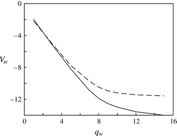
Variation of the ring voltage about its value in the absence of droplets,
 $V_{sc}={\it\varphi}-{\it\varphi}_{h}$
at (
 $x_{0},r_{0}$
), as a function of
 $q_{w}$
with
 $I_{i}=0$
. The solid curve is for the base case defined above (3.1). The dashed curve is for a flow rate of liquid equal to 1.5625 times that of the base case, for which, according to the scaling laws for an electrospray in the cone–jet mode (Fernández de la Mora Reference Fernández de la Mora2007), the values of (
 $a_{0},{\it\Phi},e_{0}$
) should be multiplied by the factors (
 $1.25,0.8,1.5625$
).

Inspection of the numerical results shows that the electric field induced by the charged droplets points away from the extractor in the whole region between this disk and the ring; in particular, a significant contribution is due to the droplets that accumulate around the line of charge that models the ring, as revealed by the accumulation of contours of constant droplet number density in figure 4. Thus, for a given value of
 $q_{w}$
, the presence of charged droplets decreases the ring’s voltage below its value in the absence of space charge. The ring’s voltage referred to that of the ring in the absence of droplets,
 $V_{sc}={\it\varphi}-{\it\varphi}_{h}$
at (
 $x_{0},r_{0}$
), is shown in figure 5 as a function of
 $q_{w}$
. As can be seen,
 $V_{sc}$
first decreases linearly with
 $q_{w}$
and tends to saturate for large values of this parameter, showing that the effect of
 $q_{w}$
on the charge distribution of the spray and on the field induced by this charge can only be increased to a certain extent.
Using again dimensional variables, the charge per unit length of the spray plume is of order
 ${\it\Gamma}=I_{d}/v_{de}$
, with
 $v_{de}\sim e_{0}E_{h}/c_{f}$
from the balance of drag and electric force. The axial field induced by this charge is of order
 $E_{d}={\it\Gamma}/{\it\epsilon}_{0}L$
(Hinch Reference Hinch1991), which is of the order of the applied field
 $E_{h}$
when
 $E_{h}\sim (c_{f}I_{d}/{\it\epsilon}_{0}e_{0}L)^{1/2}$
, or
 $E_{h}\sim 1/{\it\Pi}^{1/2}$
in dimensionless variables. Saturation should be expected for values of
 $E_{h}$
(or
 $q_{w}$
) larger than this.
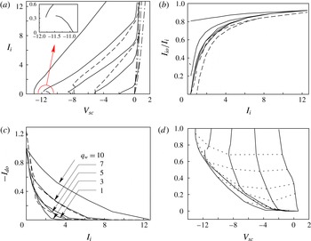
(a) Current–voltage characteristic of the corona (solid). Dash-dotted curves are the corona characteristic in the absence of droplets for
 $q_{w}=1$
, 3 and 5. The inset is a magnified view of the fold for
 $q_{w}=7$
. (b) Fraction of the ionic current that reaches the extractor and collector disks (
 $I_{io}/I_{i}$
) as a function of the total ionic current. (c) Absolute value of the electric current due to charged droplets that reach the extractor and collector disks (
 $-I_{do}$
) as a function of the ionic current. (d) Absolute value of the electric current due to charged droplets that reach the extractor and collector disks as a function of the ring’s voltage. Dotted curves are contours of constant ionic current,
 $I_{i}=0.314$
, 0.628, 1.257, 1.885, 4.398 and 8.796, increasing from top to bottom. Results are shown for
 $q_{w}=1$
, 3, 5, 7 and 10, increasing from bottom to top in (a) and (b), and from right to left in (d). Dashed curves in (a), (b) and (c) are results for a flow rate of liquid equal to 1.5625 times that of the base case, with
 $q_{w}=3$
and 5.

3.3 Corona in the presence of droplets; neutralization
The solid curves in figure 6(a) are the current–voltage characteristics of the corona in the presence of charged droplets for various values of
 $q_{w}$
. The ring’s voltage relative to the corona threshold value without droplets,
 $V_{sc}={\it\varphi}-{\it\varphi}_{h}$
at (
 $x_{0},r_{0}$
), is shown on the horizontal axis. The dash-dotted curves on the right-hand side of figure 6(a) are the characteristics of the corona without droplets, which appear as steep, nearly straight lines at the scale of the figure. Since the charged droplets are responsible for the decrease of the ring’s voltage below the corona threshold value (
 ${\it\varphi}_{h}$
at the wire), the actual characteristics tend to the characteristics without droplets when the spray is fully neutralized. The large range of voltages over which neutralization occurs, compared to the voltage variation about the threshold value that would lead to a similar current in the absence of droplets, reflects the strong effect of the droplets on the corona.
Figure 6(b) shows the fraction of the ionic current that is not used for neutralization and ends up at the extractor and collector disks,
 $I_{io}/I_{i}$
. Figure 6(c,d) shows the electric current due to the charged droplets that reach the extractor and the collector,
 $I_{do}$
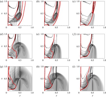
, as a function of the ionic current and of the ring’s voltage, respectively. Finally, figure 7 shows the number density of droplets (black contours), the charge density of ions (grey levels) and the region (bounded by the red contour) where the mean charge of the droplets is above half its initial value, for various values of
 $q_{w}$
and
 $I_{i}$
.
Number density of droplets (10 black contours equispaced between 0 and 60), charge density of ions (10 grey levels between 0 (white) and 5 (darkest)), and region (bounded by the red contour, or the two red contours in (a)–(c)) where the mean charge of the droplets,
 ${\it\rho}_{d}/n_{d}=\sum e_{j}/\sum 1_{j}$
, which is equal to unity at injection, stays above 0.5. Results are shown for
 $q_{w}=3$
, 5 and 7, increasing from left to right, and
 $I_{i}=0.314$
, 1.257 and 3.142, increasing from top to bottom. (a)
 $q_{w}=3$
,
 $I_{i}=0.314$
; (b)
 $q_{w}=5$
,
 $I_{i}=0.314$
; (c)
 $q_{w}=7$
,
 $I_{i}=0.314$
; (d)
 $q_{w}=3$
,
 $I_{i}=1.257$
; (e)
 $q_{w}=3$
,
 $I_{i}=1.257$
; (f)
 $q_{w}=3$
,
 $I_{i}=1.257$
; (g)
 $q_{w}=3$
,
 $I_{i}=3.142$
; (h)
 $q_{w}=5$
,
 $I_{i}=3.142$
; (i)
 $q_{w}=7$
,
 $I_{i}=3.142$
.

As can be seen in figure 7, when
 $I_{i}$
increases, neutralization first occurs at or near the shroud of the spray plume and then extends to deeper layers. The number density of droplets is high at the shroud, where the droplets that have been neutralized are no longer accelerated by the electric field and merely follow the weak gas flow.
The width of the spray decreases when
 $q_{w}$
or
 $I_{i}$
increases, as this increases the electric field acting on the droplets. The spread of the injected ions and the rate of droplet neutralization increase with
 $I_{i}$
. Some ions drift upwards and reach the collector disk when
 $I_{i}$
is higher than a certain critical value that increases with
 $q_{w}$
. The spread of the ions decreases with increasing
 $q_{w}$
, as this increases the drift velocity of the ions.
In some cases, when some droplets fly back towards the extractor disk or this condition is approached, the region of upward-pointing field around the inlet orifice mentioned in § 3.2 appears. The ions cannot reach this region, and the droplets in it are not neutralized. If these droplets fly back, they hit the extractor un-neutralized, contributing to
 $I_{do}$
. The size of the region of upward-pointing field, and the tendency of the charged droplets to fly back, are reduced or disappear when
 $q_{w}$
or
 $I_{i}$
increase; see figure 7.
The ionic current needed to neutralize the spray increases with
 $q_{w}$
(figure 6
a) because an increasing fraction of the ionic current goes directly to the extractor without entering the spray; see figure 7. This is due to the decrease of the spray width commented on above and to the increase of the downward velocity of the ions caused by the increased electric field. For the same reason, when the ionic current increases at constant
 $q_{w}$
, the fraction of this current that is not attached by droplets increases (figures 6
b and 7). In agreement with these results, the rate at which the absolute value of the electric current due to the charged droplets reaching the disks decreases with increasing
 $I_{i}$
is highest for
 $q_{w}=3$
and decreases when this parameter increases (figure 6
c). The absolute value of the droplet current is somewhat larger for
 $q_{w}=1$
than for
 $q_{w}=3$
due to the difficulty of neutralizing droplets in the region of upward-pointing field around the inlet, which is larger for
 $q_{w}=1$
than for larger values of this parameter.
The curves in figure 6(d), giving the relation between the electric current due to the charged droplets,
 $I_{do}$
, and the voltage variation of the ring,
 $V_{sc}$
, are C-shaped for
 $q_{w}=5$
and 7. In addition, the curve for
 $q_{w}=7$
has a fold with two branches that might be connected by another branch of unstable solutions, though this cannot be computed with the time marching method used here. These features are in contrast to the monotonic
 $I_{do}$
–
 $I_{i}$
relation in figure 6(c) and can be traced to similar features of the characteristics in figure 6(a) at small values of the ionic current. The results can be understood by noticing that two effects compete when a small ionic current is injected. On the one hand, the injected ions partially neutralize the droplets that were responsible for the decrease of the ring’s voltage, so that this voltage is expected to increase with
 $I_{i}$
, as discussed above. On the other hand, the presence of ions around the ring qualitatively amounts to increasing
 $q_{w}$
, which, as discussed in § 3.2, would lead to a reduction of the ring voltage in the absence of other effects of the injected ions. At small values of
 $I_{i}$
, the second effect dominates for moderate values of
 $q_{w}$
, when the slope of the
 $V_{sc}$
–
 $q_{w}$
relation in figure 5 is high, while the first effect dominates for larger values of
 $q_{w}$
, when this slope is lower. In any case, the effect of droplet neutralization dominates, and the voltage of the ring increases with
 $I_{i}$
, when this current is further increased. This explains the initial decrease of the ring voltage with increasing
 $I_{i}$
in figure 6(a) for
 $q_{w}=5$
and 7 but not for
 $q_{w}=10$
. The effect of droplet neutralization probably dominates for any
 $I_{i}$
when
 $q_{w}=1$
or 3, leading to a ring voltage that increases monotonically with
 $I_{i}$
, because the ring is then well inside the spray plume, where any ionic current injected is very efficient at neutralizing droplets.
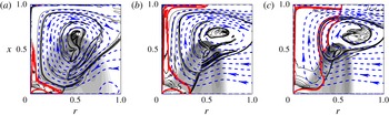
Number density of droplets (10 black contours equispaced between 0 and 400 in (a) and between 0 and 200 in (b) and (c)), charge density of ions (10 grey levels between 0 (white) and 5 (darkest)), and streamlines of the flow (dashed, with arrows), for
 $I_{i}=1.257$
,
 $v_{g_{I}}=0$
and
 $q_{w}=3$
(a), 5 (b) and 7 (c). Droplets with mean charge above half its initial value are confined to the region bounded by the red contour. Other parameters have the values (3.1).

Additional computations have been carried out without gas injection (
 $v_{g_{I}}=0$
). Some results are shown in figure 8 for
 $I_{i}=1.257$
and
 $q_{w}=3$
(a), 5 (b) and 7 (c). As can be seen, the flow induced between the disks by the entrainment of the spray plume overcomes the ionic wind; compare the streamlines in figure 8 and in figure 3(a). Clean gas flows in through the lower part of the open boundary and out through the upper part, loaded with neutralized droplets. There is a recirculation region where the number density of neutralized droplets is high, and in some cases droplets accumulate in this region and may invalidate the assumption of a dilute spray. The distribution of corona ions is not affected by these changes; compare figures 8(a–c) and 7(d–f).
The inlet conditions of the spray have been changed to study their effect on the neutralization process. In the cone–jet mode of an electrospray, the electric current carried by the droplets is proportional to the square root of the flow rate, while the radius of the droplets increases approximately as a power of the flow rate with an exponent that is not far from
 $1/2$
(see Fernández de la Mora Reference Fernández de la Mora2007). Thus, using a subscript
 $b$
to denote conditions of the base case considered up to this point, the following relations hold when these conditions are changed:
 $a_{0}/a_{0b}={\it\Phi}_{b}/{\it\Phi}=(e_{0}/e_{0b})^{1/2}=(Q/Q_{b})^{1/2}$
. Some results for
 $Q/Q_{b}=1.5625$
are included in figures 5 and 6 (dashed curves), where, to facilitate comparison, the results are non-dimensionalized with the magnitudes of the base case introduced above (3.1). In particular, the leftmost dashed curve in figure 6(a), for
 $q_{w}=5$
, has three turning points at
 $(V_{sc},I_{i})=(-7.85,0.45),(-7.73,0.97)$
and (
 $-7.98$
, 1.26).
Neutralization experiments with coronas often display unsteady neutralization regions that move across a large fraction of the spray plume and set serious limitations to the practical use of this neutralization method. These unsteady regions did not appear in the numerical simulations. While further research is needed to ascertain the cause of the difference, it may be conjectured that unsteady effects have been suppressed by the model of the corona, which uses the corona current
 $I_{i}$
as a control parameter that is kept constant instead of the voltage of the wire ring. If this is correct, and if the fluctuations of the corona current at constant voltage are determined by the slow dynamics of the whole spray, then unsteady effects could perhaps be reduced by limiting the fluctuations of the corona current.
4 Conclusions
The neutralization of a dilute spray of electrically charged droplets by ions of the opposite polarity generated by a corona discharge at a wire ring coaxial with the spray has been analysed using a model that includes: (i) a Lagrangian description of the dynamics of the droplets by means of a method of particles that accounts for electric and hydrodynamic forces and attachment of corona ions by field charging; (ii) an Eulerian, mesoscale description of the flow of the gas under the action of the forces exerted by the droplets and the ions; (iii) a conservation equation for the ions that are generated at the corona and removed by attachment to the droplets; and (iv) a Poisson equation for the electric potential that accounts for the space charge of the droplets and the ions. A line of charge surrounded by a distribution of ion sources is used to simulate the corona.
Computations carried out in the absence of droplets show that the simple, two-parameter model of the corona captures typical features of a corona’s current–voltage characteristic, and that the ionic wind induced by the force of the ions on the gas can be overcome by a weak forced flow in the range of ionic current of interest for neutralization.
In the absence of corona discharge, the field induced by the charge of the droplets opposes the applied field and leads to a reduction of the electric potential of the ring for a given value of the electric field at its surface. The velocity of the droplets increases, and the cross-section of the spray and the tendency for the droplets to fly back towards the extractor disk decrease when the electric field at the ring is increased.
The fraction of the spray charge that is neutralized before the droplets reach the metallic disks bounding the system is an increasing function of the corona current, but the value of this current required for complete neutralization is several times larger than the initial current carried by the spray because a fraction of the corona current is lost to the metallic disks. This fraction increases with the threshold voltage of the corona (which is a measure of the radius of the wire) and with the corona current itself. Moderate values of these two variables cause the corona discharge to occur within the spray plume for the configuration analysed, thereby increasing the rate of ion attachment to the droplets. However, too small values of these variables cause some of the droplets to fly back towards the extractor disk before they can be neutralized. The current–voltage characteristic of the corona is significantly affected by the presence of charged droplets, and may become multivalued for small values of the corona current.
Acknowledgement
This work was supported by the Spanish MINECO through projects DPI2013-47372-C02-02 and CSD2010-00011.