1. Introduction
Inertial particles that are initially uniformly distributed throughout an incompressible turbulent flow will develop into dynamically evolving spatial clusters. Early studies observed that inertial particles not only cluster but preferentially concentrate in strain-dominated regions of the turbulent fluid velocity field, away from regions of strong rotation (Maxey & Corrsin Reference Maxey and Corrsin1986; Maxey Reference Maxey1987; Squires & Eaton Reference Squires and Eaton1991; Wang & Maxey Reference Wang and Maxey1993; Eaton & Fessler Reference Eaton and Fessler1994; Sundaram & Collins Reference Sundaram and Collins1997). Here and throughout, we make a distinction between the terms ‘clustering’ and ‘preferential concentration,’ where the former refers to the non-uniform distribution of the particles in space, irrespective of where they cluster, and the latter refers to the clustering of particles in high strain, low-rotation regions of the flow. The reason for making this distinction is that clustering can occur without preferential concentration, a scenario that we discuss later in the paper.
The traditional explanation for the mechanism of clustering is due to Maxey (Reference Maxey1987), who argued that particles are centrifuged out of regions where the fluid streamlines exhibit strong curvature into regions of high strain. This physical argument, aside from being intuitive, explains the preferential concentration effect. However, over time the completeness of this explanation for clustering has been questioned. For example, Bec (Reference Bec2003) described simulations of particles in white-in-time random flows that exhibited strong clustering, yet the centrifuge mechanism does not operate in such flows.
In a recent paper, Bragg & Collins (Reference Bragg and Collins2014) considered in detail the physical mechanism responsible for the clustering of inertial particles in the dissipation range of isotropic turbulence. We showed that in the regime
 $St\ll 1$
(where
 $St\equiv {\it\tau}_{p}/{\it\tau}_{{\it\eta}}$
is the Stokes number,
 ${\it\tau}_{p}$
is the particle response time and
 ${\it\tau}_{{\it\eta}}$
is the Kolmogorov time scale), the mechanism for clustering predicted by the Zaichik & Alipchenkov theory (Zaichik & Alipchenkov Reference Zaichik and Alipchenkov2003, Reference Zaichik and Alipchenkov2007, Reference Zaichik and Alipchenkov2009, hereafter ZT) is the same as that predicted by the Chun et al. theory (Chun et al.
Reference Chun, Koch, Rani, Ahluwalia and Collins2005, hereafter CT), which is essentially an extension of the classical centrifuge mechanism of Maxey (Reference Maxey1987). As
 $St$
is increased beyond this regime (i.e.
 $St\geqslant O(1)$
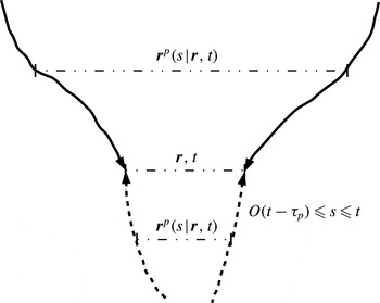
), the system undergoes a bifurcation and the particle velocity dynamics become non-local (by ‘non-local’ we mean that the particle velocity at a given time depends upon its interactions with the turbulent fluid velocity field at earlier times along its path history), and we showed that this non-locality contributes to the inward drift mechanism described by the ZT through a path history symmetry breaking effect. Figure 1 illustrates two particle-pair trajectories passing through separation
 $\boldsymbol{r}$
at time
 $t$
. For
 $St\geqslant O(1)$
, the particles retain a finite memory of their interaction with the turbulence along their path histories, over a timeframe
 $O(t-{\it\tau}_{p})\leqslant s\leqslant t$
. The particle pair separation is given by
 $\boldsymbol{r}^{p}(s\mid \boldsymbol{r},t)$
, where
 $\boldsymbol{r}^{p}$
is the time-dependent separation, and
 $|\boldsymbol{r},t$
denotes that the pair has separation
 $\boldsymbol{r}$
at time
 $t$
. For the solid line trajectories in figure 1,
 $\boldsymbol{r}^{p}(s\mid \boldsymbol{r},t)\geqslant \boldsymbol{r}$
and for the dashed line trajectories,
 $\boldsymbol{r}^{p}(s\mid \boldsymbol{r},t)\leqslant \boldsymbol{r}$
. Since the fluid velocity difference,
 ${\rm\Delta}\boldsymbol{u}$
, on average increases with separation then particle pairs with
 $\boldsymbol{r}^{p}(s\mid \boldsymbol{r},t)\geqslant \boldsymbol{r}$
will have experienced, on average, larger values of
 ${\rm\Delta}\boldsymbol{u}$
in their path history as compared with particle pairs with
 $\boldsymbol{r}^{p}(s\mid \boldsymbol{r},t)\leqslant \boldsymbol{r}$
. This asymmetry in the particle pairs’ path histories breaks the symmetry of their inward and outward motions and gives rise to a net inward drift, leading to clustering. Note that the origin of this path history clustering mechanism is intimately connected to that which gives rise to the ‘sling effect’ (Falkovich, Fouxon & Stepanov Reference Falkovich, Fouxon and Stepanov2002; Falkovich & Pumir Reference Falkovich and Pumir2007) and ‘caustics’ (Wilkinson & Mehlig Reference Wilkinson and Mehlig2005).
We also argued that the theory for clustering in Gustavsson & Mehlig (Reference Gustavsson and Mehlig2011b
) is qualitatively similar to that in the ZT in the regimes
 $St\ll 1$
and
 $St\gg 1$
. The non-local, path history symmetry breaking mechanism in the ZT and the non-local ‘ergodic mechanism’ in Gustavsson & Mehlig (Reference Gustavsson and Mehlig2011b
) both explain the clustering in white-in-time flows observed in Bec (Reference Bec2003). Note that the ZT is more general in its description, as it applies to all
 $St$
and correlation time scales for the fluid, whereas Gustavsson & Mehlig (Reference Gustavsson and Mehlig2011b
) treat these time scales as a small parameter.
There is however an outstanding issue that remains to be explained. Bragg & Collins (Reference Bragg and Collins2014) showed that the non-local clustering mechanism in the ZT makes the dominant contribution when
 $St=O(1)$
(see figure 3 in Bragg & Collins (Reference Bragg and Collins2014) and the surrounding discussion). However, we also know from numerical simulations (e.g. Squires & Eaton Reference Squires and Eaton1991) that at
 $St=O(1)$
there exist strong correlations between the location of the clusters and the local topology of the fluid velocity gradient field, i.e. preferential concentration. In the regime
 $St\ll 1$
, the phenomenon of preferential concentration is easily explained since the mechanism generating the clustering depends upon the preferential sampling of the local fluid velocity gradient (Chun et al.
Reference Chun, Koch, Rani, Ahluwalia and Collins2005; Balachandar & Eaton Reference Balachandar and Eaton2010). However, for
 $St=O(1)$
the clustering mechanism is strongly non-local, and this symmetry breaking clustering mechanism does not explicitly depend upon the local flow topology. How then does the non-local clustering mechanism continue to generate preferential concentration? In this paper, we address this question through an analysis of the exact equation for the radial distribution function (RDF), an important measure of clustering. In particular, we resolve the issue by showing that the non-local clustering mechanism is influenced by the preferential sampling of
 ${\it\bf\Gamma}$
, the fluid velocity gradient tensor, along the path histories of the particles in such a way as to generate stronger inward drift velocities into regions where
 ${\it\bf\Gamma}$
at the current particle position exhibits high strain and low-rotation. Our analysis also shows how in flows where the centrifuge mechanism does not operate and the preferential sampling effect is absent, the non-local mechanism generates clustering without preferential concentration.
Illustration of two particle-pair trajectories arriving at separation
 $\boldsymbol{r}$
at time
 $t$
. The solid lines represent a pair of particle trajectories with separation
 $\boldsymbol{r}^{p}(s\mid \boldsymbol{r},t)\geqslant \boldsymbol{r}$
and the dashed lines a pair with
 $\boldsymbol{r}^{p}(s\mid \boldsymbol{r},t)\leqslant \boldsymbol{r}$
.

2. Theoretical analysis
2.1. Derivation of the drift velocity conditioned on the local flow structure
We consider the relative motion between two identical point particles, a ‘primary’ particle and a ‘satellite’ particle, the primary particle being the reference particle. The particles experience Stokes drag forces, but do not interact with each other through physical collisions or hydrodynamic interactions and are assumed to be at low enough concentration to not affect the turbulence (i.e. ‘one-way coupling’). The turbulence is assumed to be statistically stationary, homogeneous and isotropic, and gravitational settling is neglected. The particle-to-fluid density ratio is large, corresponding to a gas–solid system. Under these assumptions, the equation governing the motion of the particles reduces to (Maxey & Riley Reference Maxey and Riley1983)
 $$\begin{eqnarray}\dot{\boldsymbol{v}}^{p}(t)=(St\,{\it\tau}_{{\it\eta}})^{-1}(\boldsymbol{u}(\boldsymbol{x}^{p}(t),t)-\boldsymbol{v}^{p}(t)),\end{eqnarray}$$
where
 $\boldsymbol{x}^{p}(t),\boldsymbol{v}^{p}(t)$
and
 $\dot{\boldsymbol{v}}^{p}(t)$
are the particle position, velocity and acceleration vectors, and
 $\boldsymbol{u}(\boldsymbol{x}^{p}(t),t)$
is the fluid velocity evaluated at the particle position. The equation governing the relative motion of two physically identical particles, each of which is governed by (2.1), is then given by
 $$\begin{eqnarray}\dot{\boldsymbol{w}}^{p}(t)=(St\,{\it\tau}_{{\it\eta}})^{-1}({\rm\Delta}\boldsymbol{u}(\boldsymbol{x}^{p}(t),\boldsymbol{r}^{p}(t),t)-\boldsymbol{w}^{p}(t)),\end{eqnarray}$$
where
 $\boldsymbol{r}^{p}(t),\boldsymbol{w}^{p}(t)$
and
 $\dot{\boldsymbol{w}}^{p}(t)$
are the particle pair relative separation, velocity and acceleration vectors, respectively,
 $\boldsymbol{x}^{p}(t)$
denotes the primary particle (reference particle) position and
 ${\rm\Delta}\boldsymbol{u}(\boldsymbol{x}^{p}(t),\boldsymbol{r}^{p}(t),t)$
is the difference in the fluid velocity evaluated at the positions of the two particles. Since we are interested in the case where
 $\boldsymbol{u}(\boldsymbol{x},t)$
is statistically homogeneous, we shall drop the
 $\boldsymbol{x}^{p}(t)$
argument when
 ${\rm\Delta}\boldsymbol{u}$
appears in statistical expressions.
For the system governed by (2.2) the exact equation governing the probability density function (PDF),
 $$\begin{eqnarray}p(\boldsymbol{r},\boldsymbol{w},t)\equiv \langle {\it\delta}(\boldsymbol{r}^{p}(t)-\boldsymbol{r}){\it\delta}(\boldsymbol{w}^{p}(t)-\boldsymbol{w})\rangle ,\end{eqnarray}$$
describing the distribution of
 $\boldsymbol{r}^{p}(t),\boldsymbol{w}^{p}(t)$
, in the phase space
 $\boldsymbol{r},\boldsymbol{w}$
is
 $$\begin{eqnarray}\partial _{t}p=-\boldsymbol{{\rm\nabla}}_{\boldsymbol{r}}\boldsymbol{\cdot }p\boldsymbol{w}+(St\,{\it\tau}_{{\it\eta}})^{-1}\boldsymbol{{\rm\nabla}}_{\boldsymbol{ w}}\boldsymbol{\cdot }p\boldsymbol{w}-(St\,{\it\tau}_{{\it\eta}})^{-1}\boldsymbol{{\rm\nabla}}_{\boldsymbol{ w}}\boldsymbol{\cdot }p\left\langle {\rm\Delta}\boldsymbol{u}(\boldsymbol{r}^{p}(t),t)\right\rangle _{\boldsymbol{ r},\boldsymbol{w}}\!,\end{eqnarray}$$
where
 $\langle \cdot \rangle _{\boldsymbol{r},\boldsymbol{w}}$
denotes an ensemble average conditioned on
 $\boldsymbol{r}^{p}(t)=\boldsymbol{r}$
and
 $\boldsymbol{w}^{p}(t)=\boldsymbol{w}$
. A commonly used statistical measure of particle clustering is the radial distribution function (RDF, McQuarrie Reference McQuarrie1976), which is defined as the ratio of the number of particle pairs at separation
 $\boldsymbol{r}$
to the number that would be expected if the particles were uniformly distributed. An exact equation for the statistically stationary RDF,
 $g(\boldsymbol{r})$
, can be constructed by multiplying the stationary form of (2.4) by
 $\boldsymbol{w}$
and then integrating over all
 $\boldsymbol{w}$
yielding (see appendix A for details)
 $$\begin{eqnarray}\mathbf{0}=g\langle {\rm\Delta}\boldsymbol{u}(\boldsymbol{r}^{p}(t),t)\rangle _{\boldsymbol{ r}}-St\,{\it\tau}_{{\it\eta}}\boldsymbol{S}_{2}^{p}\boldsymbol{\cdot }\boldsymbol{{\rm\nabla}}_{\boldsymbol{ r}}g-St\,{\it\tau}_{{\it\eta}}g\boldsymbol{{\rm\nabla}}_{\boldsymbol{r}}\boldsymbol{\cdot }\boldsymbol{S}_{2}^{p},\end{eqnarray}$$
where
 $$\begin{eqnarray}g(\boldsymbol{r})=\frac{N(N-1)}{n^{2}V}\int _{\boldsymbol{w}}p(\boldsymbol{r},\boldsymbol{w})\,\text{d}\boldsymbol{w},\end{eqnarray}$$
 $N$
is the total number of particles lying within the control volume
 $V$
,
 $n\equiv N/V$
is the number density of particles and
 $\boldsymbol{S}_{2}^{p}(\boldsymbol{r})\equiv \langle \boldsymbol{w}^{p}(t)\boldsymbol{w}^{p}(t)\rangle _{\boldsymbol{r}}$
is the second-order particle velocity structure function.
Equation (2.5) is exact, but unclosed, due to the term
 $\langle {\rm\Delta}\boldsymbol{u}(\boldsymbol{r}^{p}(t),t)\rangle _{\boldsymbol{r}}$
which describes the average of
 ${\rm\Delta}\boldsymbol{u}$
experienced by particle pairs at the separation
 $\boldsymbol{r}^{p}(t)=\boldsymbol{r}$
. Even though
 $\langle {\rm\Delta}\boldsymbol{u}(\boldsymbol{r},t)\rangle =\mathbf{0}$
for isotropic flows,
 $\langle {\rm\Delta}\boldsymbol{u}(\boldsymbol{r}^{p}(t),t)\rangle _{\boldsymbol{r}}\neq \mathbf{0}$
for finite
 $St$
because the inertial particles preferentially sample the underlying field
 ${\rm\Delta}\boldsymbol{u}(\boldsymbol{x},\boldsymbol{r},t)$
. In the ZT, this term is closed by approximating
 ${\rm\Delta}\boldsymbol{u}(\boldsymbol{x},\boldsymbol{r},t)$
as a spatio-temporally correlated Gaussian field and using the Furutsu–Novikov closure method (Zaichik & Alipchenkov Reference Zaichik and Alipchenkov2007; Bragg & Collins Reference Bragg and Collins2014). However, for the purposes of this analysis, it is not necessary to introduce any such closure approximations. Recall that the purpose of this analysis is to demonstrate that the non-local clustering mechanism, which dominates at
 $St=O(1)$
, is consistent with the phenomenon of preferential concentration. It is unnecessary to close
 $\langle {\rm\Delta}\boldsymbol{u}(\boldsymbol{r}^{p}(t),t)\rangle _{\boldsymbol{r}}$
for two reasons. First, Bragg & Collins (Reference Bragg and Collins2014) showed that at
 $St=O(1)$
the drift velocity contributions coming from
 $\langle {\rm\Delta}\boldsymbol{u}(\boldsymbol{r}^{p}(t),t)\rangle _{\boldsymbol{r}}$
are negligible compared to the drift mechanism associated with
 $St\,{\it\tau}_{{\it\eta}}\boldsymbol{{\rm\nabla}}_{\boldsymbol{r}}\boldsymbol{\cdot }\boldsymbol{S}_{2}^{p}$
in (2.5). The reason for this is that at
 $St=O(1)$
in the dissipation range of the turbulence, the particle relative velocities exhibit ‘caustics’ (Wilkinson & Mehlig Reference Wilkinson and Mehlig2005; Bec et al.
Reference Bec, Biferale, Cencini, Lanotte and Toschi2010; Salazar & Collins Reference Salazar and Collins2012b
), which implies they are much larger than the fluid relative velocities. A consequence of this is that contributions to the particle relative motion coming from their local interaction with the turbulence (e.g.
 ${\rm\Delta}\boldsymbol{u}(\boldsymbol{r}^{p}(t),t)$
) become negligible. Second, any contributions to the clustering mechanism associated with
 $\langle {\rm\Delta}\boldsymbol{u}(\boldsymbol{r}^{p}(t),t)\rangle _{\boldsymbol{r}}$
are manifestly consistent with the phenomenon of preferential concentration since this term arises because of preferential sampling effects.
The challenge therefore is to show that the drift velocity
 $St\,{\it\tau}_{{\it\eta}}\boldsymbol{{\rm\nabla}}_{\boldsymbol{r}}\boldsymbol{\cdot }\boldsymbol{S}_{2}^{p}$
, which generates the clustering and is strongly non-local at
 $St=O(1)$
, is consistent with the phenomenon of preferential concentration. The physical interpretation of
 $St\,{\it\tau}_{{\it\eta}}\boldsymbol{{\rm\nabla}}_{\boldsymbol{r}}\boldsymbol{\cdot }\boldsymbol{S}_{2}^{p}$
has already been discussed in the introduction. We refer the reader to Bragg & Collins (Reference Bragg and Collins2014) for a more detailed explanation.
Since we are interested in clustering in the dissipation range we take
 $$\begin{eqnarray}{\rm\Delta}\boldsymbol{u}(\boldsymbol{x}^{p}(t),\boldsymbol{r}^{p}(t),t)={\it\bf\Gamma}(\boldsymbol{x}^{p}(t),t)\boldsymbol{\cdot }\boldsymbol{r}^{p}(t),\end{eqnarray}$$
where
 ${\it\bf\Gamma}(\boldsymbol{x},t)\equiv \boldsymbol{{\rm\nabla}}_{\boldsymbol{x}}\boldsymbol{u}(\boldsymbol{x},t)$
is the fluid velocity gradient tensor. If the non-local clustering mechanism for particles with
 $St=O(1)$
is consistent with the phenomenon of preferential concentration, then it must be the case that contributions to
 $St\,{\it\tau}_{{\it\eta}}\boldsymbol{{\rm\nabla}}_{\boldsymbol{r}}\boldsymbol{\cdot }\boldsymbol{S}_{2}^{p}$
are larger for particles that are (at present time,
 $t$
) sitting in high strain, low-rotation regions than they are for particles sitting in high-rotation, low strain regions of the flow field.
In order to formally consider this possibility, we expand the phase space description of the drift velocity as shown below
 $$\begin{eqnarray}-St\,{\it\tau}_{{\it\eta}}\boldsymbol{{\rm\nabla}}_{\boldsymbol{r}}\boldsymbol{\cdot }\boldsymbol{S}_{2}^{p}\equiv \int _{\mathscr{ Z}}{\it\varrho}(\mathscr{Z})\underbrace{\left\{-St\,{\it\tau}_{{\it\eta}}\boldsymbol{{\rm\nabla}}_{\boldsymbol{r}}\boldsymbol{\cdot }\left\langle \boldsymbol{w}^{p}(t)\boldsymbol{w}^{p}(t)\right\rangle _{\boldsymbol{ r},\mathscr{Z}}\right\}}_{\mathit{Drift}\,\mathit{velocity}\,\mathit{conditioned}\,\mathit{on}\,\mathscr{Z}^{p}(t,t)=\mathscr{Z}}\text{d}\mathscr{Z},\end{eqnarray}$$
where
 $\mathscr{Z}$
is an independent phase space variable,
 ${\it\varrho}(\mathscr{Z})\equiv \langle {\it\delta}(\mathscr{Z}^{p}(t,t)-\mathscr{Z})\rangle$
,
 $\mathscr{Z}^{p}(t^{\prime },t^{\prime \prime })\equiv \mathbf{\mathscr{S}}(\boldsymbol{x}^{p}(t^{\prime }),t^{\prime })\boldsymbol{ : }\mathbf{\mathscr{S}}(\boldsymbol{x}^{p}(t^{\prime \prime }),t^{\prime \prime })-\mathbf{\mathscr{R}}(\boldsymbol{x}^{p}(t^{\prime }),t^{\prime })\boldsymbol{ : }\mathbf{\mathscr{R}}(\boldsymbol{x}^{p}(t^{\prime \prime }),t^{\prime \prime })$
,
 $\mathbf{\mathscr{S}}$
and
 $\mathbf{\mathscr{R}}$
are the fluid strain rate and rotation rate tensors, respectively, defined as
 $\mathbf{\mathscr{S}}\equiv (1/2)({\it\bf\Gamma}+{\it\bf\Gamma}^{\text{T}})$
,
 $\mathbf{\mathscr{R}}\equiv (1/2)({\it\bf\Gamma}-{\it\bf\Gamma}^{\text{T}})$
, and
 $\langle \cdot \rangle _{\boldsymbol{r},\mathscr{Z}}$
denotes an ensemble average conditioned on
 $\boldsymbol{r}^{p}(t)=\boldsymbol{r}$
and
 $\mathscr{Z}^{p}(t,t)=\mathscr{Z}$
. We have defined
 $\mathscr{Z}^{p}$
in terms of two time arguments
 $t^{\prime }$
and
 $t^{\prime \prime }$
since quantities appearing later in the analysis will involve the more general expression
 $\mathscr{Z}^{p}(t^{\prime },t^{\prime \prime })$
. Through (2.8) we are able to consider how the non-local contribution to the inward drift velocity is related to the local properties of
 ${\it\bf\Gamma}$
at the particles current location
 $\boldsymbol{x}^{p}(t)$
, where the relevant properties of
 ${\it\bf\Gamma}(\boldsymbol{x}^{p}(t),t)$
are characterized by its invariant
 $\mathscr{Z}^{p}(t,t)$
.
We shall now define what we mean by high strain, low-rotation regions and high-rotation, low strain regions. A rigorous definition of these regions could be given in terms of the invariants and eigenvalues of
 ${\it\bf\Gamma}(\boldsymbol{x},t)$
(e.g. Chong, Perry & Cantwell Reference Chong, Perry and Cantwell1990; Rouson & Eaton Reference Rouson and Eaton2001; Salazar & Collins Reference Salazar and Collins2012a
), however for our purposes this is not necessary. In the regime
 $St\ll 1$
, the single particle velocity
 $\boldsymbol{v}^{p}(t)$
can be approximated as being a field, i.e.
 $\boldsymbol{v}^{p}(t)\approx \boldsymbol{v}(\boldsymbol{x}^{p}(t),t)$
with a divergence
 $\boldsymbol{{\rm\nabla}}_{\boldsymbol{x}}\,\boldsymbol{\cdot }\,\boldsymbol{v}(\boldsymbol{x}^{p}(t),t)\,\approx -\!St\,{\it\tau}_{{\it\eta}}\mathscr{Z}^{p}(t,t)$
implying particles will cluster in regions where
 $\mathscr{Z}^{p}(t,t)>0$
(Maxey Reference Maxey1987), which are commonly referred to as high strain, low-rotation regions. Numerical simulations have not only confirmed this for
 $St\ll 1$
, but have shown that inertial particles continue to preferentially concentrate in
 $\mathscr{Z}^{p}(t,t)>0$
regions even when
 $St=O(1)$
. Since it is the clustering behaviour in these regions that is of interest, what we want to demonstrate is that for
 $St=O(1)$
 $$\begin{eqnarray}-St\,{\it\tau}_{{\it\eta}}\boldsymbol{{\rm\nabla}}_{\boldsymbol{r}}\boldsymbol{\cdot }\left\langle \boldsymbol{w}^{p}(t)\boldsymbol{w}^{p}(t)\right\rangle _{\boldsymbol{ r},\mathscr{Z}^{[+]}}<-St\,{\it\tau}_{{\it\eta}}\boldsymbol{{\rm\nabla}}_{\boldsymbol{r}}\boldsymbol{\cdot }\left\langle \boldsymbol{w}^{p}(t)\boldsymbol{w}^{p}(t)\right\rangle _{\boldsymbol{ r},\mathscr{Z}^{[-]}},\end{eqnarray}$$
where
 $$\begin{eqnarray}-St\,{\it\tau}_{{\it\eta}}\boldsymbol{{\rm\nabla}}_{\boldsymbol{r}}\boldsymbol{\cdot }\left\langle \boldsymbol{w}^{p}(t)\boldsymbol{w}^{p}(t)\right\rangle _{\boldsymbol{ r},\mathscr{Z}^{[+]}}\equiv \int _{0}^{+\infty }{\it\varrho}(\mathscr{Z})\left\{-St\,{\it\tau}_{{\it\eta}}\boldsymbol{{\rm\nabla}}_{\boldsymbol{ r}}\boldsymbol{\cdot }\left\langle \boldsymbol{w}^{p}(t)\boldsymbol{w}^{p}(t)\right\rangle _{\boldsymbol{ r},\mathscr{Z}}\right\}\text{d}\mathscr{Z}\end{eqnarray}$$
and
 $$\begin{eqnarray}-St\,{\it\tau}_{{\it\eta}}\boldsymbol{{\rm\nabla}}_{\boldsymbol{r}}\boldsymbol{\cdot }\left\langle \boldsymbol{w}^{p}(t)\boldsymbol{w}^{p}(t)\right\rangle _{\boldsymbol{ r},\mathscr{Z}^{[-]}}\equiv \int _{-\infty }^{0}{\it\varrho}(\mathscr{Z})\left\{-St\,{\it\tau}_{{\it\eta}}\boldsymbol{{\rm\nabla}}_{\boldsymbol{ r}}\boldsymbol{\cdot }\left\langle \boldsymbol{w}^{p}(t)\boldsymbol{w}^{p}(t)\right\rangle _{\boldsymbol{ r},\mathscr{Z}}\right\}\text{d}\mathscr{Z}.\end{eqnarray}$$
Note that by definition
 $$\begin{eqnarray}-St\,{\it\tau}_{{\it\eta}}\boldsymbol{{\rm\nabla}}_{\boldsymbol{r}}\boldsymbol{\cdot }\boldsymbol{S}_{2}^{p}\equiv -St\,{\it\tau}_{{\it\eta}}\boldsymbol{{\rm\nabla}}_{\boldsymbol{ r}}\boldsymbol{\cdot }\left\langle \boldsymbol{w}^{p}(t)\boldsymbol{w}^{p}(t)\right\rangle _{\boldsymbol{ r},\mathscr{Z}^{[+]}}-St\,{\it\tau}_{{\it\eta}}\boldsymbol{{\rm\nabla}}_{\boldsymbol{r}}\boldsymbol{\cdot }\left\langle \boldsymbol{w}^{p}(t)\boldsymbol{w}^{p}(t)\right\rangle _{\boldsymbol{ r},\mathscr{Z}^{[-]}}.\end{eqnarray}$$
The formal solution for
 $\boldsymbol{w}^{p}(t)$
for particle pairs in the dissipation range governed by (2.2) is
 $$\begin{eqnarray}\boldsymbol{w}^{p}(t)=\boldsymbol{w}^{p}(0)\text{e}^{-t/{\it\tau}_{p}}+(St\,{\it\tau}_{{\it\eta}})^{-1}\int _{0}^{t}\text{e}^{-(t-t^{\prime })/{\it\tau}_{p}}{\it\bf\Gamma}(\boldsymbol{x}^{p}(t^{\prime }),t^{\prime })\boldsymbol{\cdot }\boldsymbol{r}^{p}(t^{\prime })\,\text{d}t^{\prime }.\end{eqnarray}$$
Since we are interested in the statistically stationary state where
 $t\rightarrow \infty$
, the effect of the initial condition is
 $\lim _{t\rightarrow \infty }\boldsymbol{w}^{p}(0)\text{e}^{-t/{\it\tau}_{p}}\rightarrow 0$
and is therefore ignored. We then use (2.13) and obtain
 $$\begin{eqnarray}-St\,{\it\tau}_{{\it\eta}}\boldsymbol{{\rm\nabla}}_{\boldsymbol{r}}\boldsymbol{\cdot }\left\langle \boldsymbol{w}^{p}(t)\boldsymbol{w}^{p}(t)\right\rangle _{\boldsymbol{ r},\mathscr{Z}}=-(St\,{\it\tau}_{{\it\eta}})^{-1}\int _{0}^{t}\int _{0}^{t}\text{e}^{-(2t-t^{\prime }-t^{\prime \prime })/{\it\tau}_{p}}\boldsymbol{{\rm\nabla}}_{\boldsymbol{r}}\boldsymbol{\cdot }\boldsymbol{Q}\,\text{d}t^{\prime }\text{d}t^{\prime \prime },\end{eqnarray}$$
where the components of
 $\boldsymbol{Q}$
are
 $$\begin{eqnarray}Q_{ij}(\boldsymbol{r},\mathscr{Z},t,t^{\prime },t^{\prime \prime })\equiv \left\langle {\it\Gamma}_{im}(\boldsymbol{x}^{p}(t^{\prime }),t^{\prime })r_{m}^{p}(t^{\prime }){\it\Gamma}_{jn}(\boldsymbol{x}^{p}(t^{\prime \prime }),t^{\prime \prime })r_{n}^{p}(t^{\prime \prime })\right\rangle _{\boldsymbol{ r},\mathscr{Z}}\!.\end{eqnarray}$$
We now seek a simplification of (2.15) that is valid in the regime of interest, namely
 $St=O(1)$
and
 $r\ll {\it\eta}$
, where
 ${\it\eta}$
is the Kolmogorov length scale. Since we are interested in
 $St=O(1)$
, neither
 $St$
or
 $1/St$
can be treated as a small parameter. However in this regime, the particle velocity dynamics are strongly non-local, implying
 $\boldsymbol{w}^{p}\gg {\rm\Delta}\boldsymbol{u}$
, which is associated with the formation of caustics in the particle velocities (Wilkinson & Mehlig Reference Wilkinson and Mehlig2005; Bec et al.
Reference Bec, Biferale, Cencini, Lanotte and Toschi2010; Salazar & Collins Reference Salazar and Collins2012b
). This suggests that we can define the small parameter
 ${\it\mu}\equiv \Vert \langle {\rm\Delta}\boldsymbol{u}(\boldsymbol{r},t){\rm\Delta}\boldsymbol{u}(\boldsymbol{r},t)\rangle \Vert /\Vert \boldsymbol{S}_{2}^{p}(\boldsymbol{r})\Vert$
, which in the caustic regions satisfies
 ${\it\mu}\ll 1$
. We therefore introduce the perturbation expansion
 $$\begin{eqnarray}\boldsymbol{Q}=\boldsymbol{Q}^{[0]}+{\it\mu}\boldsymbol{Q}^{[1]}+{\it\mu}^{2}\boldsymbol{Q}^{[2]}+\cdots \,,\end{eqnarray}$$
where the components of
 $\boldsymbol{Q}^{[0]}$
are
 $$\begin{eqnarray}Q_{ij}^{[0]}=\left\langle r_{m}^{p}(t^{\prime })r_{n}^{p}(t^{\prime \prime })\right\rangle _{\boldsymbol{ r}}\left\langle {\it\Gamma}_{im}(\boldsymbol{x}^{p}(t^{\prime }),t^{\prime }){\it\Gamma}_{jn}(\boldsymbol{x}^{p}(t^{\prime \prime }),t^{\prime \prime })\right\rangle _{\mathscr{ Z}}.\end{eqnarray}$$
This expression for
 $\boldsymbol{Q}^{[0]}$
follows from the fact that in the limit
 ${\it\mu}\rightarrow 0$
the particle motion approaches ballistic motion, implying that the correlation between
 $\boldsymbol{r}^{p}$
and
 ${\it\bf\Gamma}$
vanishes, and the particles uniformly sample
 ${\it\bf\Gamma}$
. In the regime
 ${\it\mu}\ll 1$
, to leading order
 $\boldsymbol{Q}\approx \boldsymbol{Q}^{[0]}+O({\it\mu})$
, which can be used in (2.14) to construct an expression for
 $-St\,{\it\tau}_{{\it\eta}}\boldsymbol{{\rm\nabla}}_{\boldsymbol{r}}\boldsymbol{\cdot }\langle \boldsymbol{w}^{p}(t)\boldsymbol{w}^{p}(t)\rangle _{\boldsymbol{r},\mathscr{Z}}$
.
The term
 $\langle \boldsymbol{r}^{p}(t^{\prime })\boldsymbol{r}^{p}(t^{\prime \prime })\rangle _{\boldsymbol{r}}$
in (2.17) is related to the average growth of the particle pair separation
 $\boldsymbol{r}^{p}$
backward-in-time (noting that
 $t^{\prime }\leqslant t$
and
 $t^{\prime \prime }\leqslant t$
), evaluated for pair trajectories that satisfy
 $\boldsymbol{r}^{p}(t)=\boldsymbol{r}$
. For
 $t^{\prime }=t^{\prime \prime }$
the quantity is the backward-in-time mean square separation of the particle pair. The quantity may be expressed as
 $$\begin{eqnarray}\left\langle \boldsymbol{r}^{p}(t^{\prime })\boldsymbol{r}^{p}(t^{\prime \prime })\right\rangle _{\boldsymbol{ r}}\equiv \boldsymbol{r}\boldsymbol{r}+{\it\bf\Theta},\end{eqnarray}$$
where
 ${\it\bf\Theta}(\boldsymbol{r},t,t^{\prime },t^{\prime \prime })\!$
is the backward-in-time separation tensor,
 $\!$
satisfying
 ${\it\bf\Theta}(\boldsymbol{r},t,t,t)=\mathbf{0}$
. In the regime
 ${\it\mu}\ll 1$
, using the formal solution for
 $\boldsymbol{r}^{p}$
for particles governed by (2.2), we obtain the approximation (see Bragg, Ireland & Collins Reference Bragg, Ireland and Collins2014)
 $$\begin{eqnarray}{\it\bf\Theta}=(St\,{\it\tau}_{{\it\eta}})^{2}\boldsymbol{S}_{2}^{p}\left[1-\text{e}^{(t-t^{\prime })/{\it\tau}_{p}}-\text{e}^{(t-t^{\prime \prime })/{\it\tau}_{p}}+\text{e}^{(2t-t^{\prime }-t^{\prime \prime })/{\it\tau}_{p}}\right]+O({\it\mu}).\end{eqnarray}$$
The result in (2.19) is only valid for
 $\max [t-t^{\prime },t-t^{\prime \prime }]\leqslant O({\it\tau}_{p})$
since for larger time separations the process transitions into a different regime (Bragg et al.
Reference Bragg, Ireland and Collins2014). However, particles only retain a memory of their interaction with the turbulence up to times
 $O(t-{\it\tau}_{p})$
in their path history, making the approximation in (2.19) sufficient to capture the dominant contribution to the drift velocity.
Substituting (2.18) into (2.17), and taking the divergence yields
 $$\begin{eqnarray}\displaystyle \boldsymbol{{\rm\nabla}}_{r_{j}}Q_{ij} & = & \displaystyle \boldsymbol{{\rm\nabla}}_{r_{j}}[r_{m}r_{n}]\left\langle {\it\Gamma}_{im}(\boldsymbol{x}^{p}(t^{\prime }),t^{\prime }){\it\Gamma}_{jn}(\boldsymbol{x}^{p}(t^{\prime \prime }),t^{\prime \prime })\right\rangle _{\mathscr{Z}}\nonumber\\ \displaystyle & & \displaystyle +\,\boldsymbol{{\rm\nabla}}_{r_{j}}[{\it\Theta}_{mn}]\left\langle {\it\Gamma}_{im}(\boldsymbol{x}^{p}(t^{\prime }),t^{\prime }){\it\Gamma}_{jn}(\boldsymbol{x}^{p}(t^{\prime \prime }),t^{\prime \prime })\right\rangle _{\mathscr{Z}}+O({\it\mu}).\end{eqnarray}$$
Using (2.19) in this expression, substituting this into (2.14) and simplifying allows us to construct expressions for (2.10) and (2.11) that are valid for
 ${\it\mu}\ll 1$
, yielding
 $$\begin{eqnarray}\displaystyle & & \displaystyle \hspace{-10.79993pt}-St\,{\it\tau}_{{\it\eta}}\boldsymbol{{\rm\nabla}}_{\boldsymbol{r}}\boldsymbol{\cdot }\left\langle \boldsymbol{w}^{p}(t)\boldsymbol{w}^{p}(t)\right\rangle _{\boldsymbol{r},\mathscr{Z}^{[+,-]}}\nonumber\\ \displaystyle & & \displaystyle \quad =\,\underbrace{-(St\,{\it\tau}_{{\it\eta}})^{-1}\frac{\boldsymbol{r}}{3}\int _{0}^{t}\int _{0}^{t}\text{e}^{-(2t-t^{\prime }-t^{\prime \prime })/{\it\tau}_{p}}\left\langle \mathscr{Z}^{p}(t^{\prime },t^{\prime \prime })\right\rangle _{\mathscr{Z}^{[+,-]}}\,\text{d}t^{\prime }\,\text{d}t^{\prime \prime }}_{\unicode[STIX]{x2460}}\nonumber\\ \displaystyle & & \displaystyle \qquad \,\underbrace{-\,(St\,{\it\tau}_{{\it\eta}})^{-1}\frac{\boldsymbol{r}}{3}\int _{0}^{t}\int _{0}^{t}r^{-1}\boldsymbol{{\rm\nabla}}_{r}\widetilde{{\it\Theta}}_{\Vert }\left\langle \mathscr{Y}^{p}(t^{\prime },t^{\prime \prime })\right\rangle _{\mathscr{ Z}^{[+,-]}}\,\text{d}t^{\prime }\,\text{d}t^{\prime \prime }}_{\unicode[STIX]{x2461}},\end{eqnarray}$$
where
 $\mathscr{Y}^{p}(t^{\prime },t^{\prime \prime })\equiv \mathbf{\mathscr{S}}(\boldsymbol{x}^{p}(t^{\prime }),t^{\prime })\boldsymbol{ : }\mathbf{\mathscr{S}}(\boldsymbol{x}^{p}(t^{\prime \prime }),t^{\prime \prime })+\mathbf{\mathscr{R}}(\boldsymbol{x}^{p}(t^{\prime }),t^{\prime })\boldsymbol{ : }\mathbf{\mathscr{R}}(\boldsymbol{x}^{p}(t^{\prime \prime }),t^{\prime \prime })$
,
 $\widetilde{{\it\Theta}}_{\Vert }(r,t,t^{\prime },t^{\prime \prime })\equiv r^{-2}\boldsymbol{r}\boldsymbol{r}\boldsymbol{ : }{\it\bf\Theta}(\boldsymbol{r},-t,-t^{\prime },-t^{\prime \prime })$
, and we have introduced the approximation in
 ${\it\bf\Theta}$
that
 $\boldsymbol{S}_{2}^{p}\approx S_{2\Vert }^{p}\mathbf{I}$
, which is valid for
 $St\geqslant O(1)$
(Wang, Wexler & Zhou Reference Wang, Wexler and Zhou2000). The notation
 $\mathscr{Z}^{[+,-]}$
in (2.21) denotes that the conditionality is either to be taken as
 $\mathscr{Z}^{[+]}$
or
 $\mathscr{Z}^{[-]}$
. For an isotropic system, the drift velocity between the particles is given by the projection of (2.21) along
 $r^{-1}\boldsymbol{r}$
such that the drift velocity only depends on
 $r=\Vert \boldsymbol{r}\Vert$
and not the vector
 $\boldsymbol{r}$
. Consequently, the sign of
 $\boldsymbol{r}$
in (2.21) is irrelevant in the following discussion.
The physical interpretation of terms
 $\unicode[STIX]{x2460}$
and
 $\unicode[STIX]{x2461}$
may be explained as follows. Suppose that during the particle time scale,
 ${\it\tau}_{p}$
, the pair separation
 $\boldsymbol{r}^{p}$
remains almost constant. In this case term
 $\unicode[STIX]{x2461}$
would vanish (because
 $\widetilde{{\it\Theta}}_{\Vert }$
and
 $\boldsymbol{{\rm\nabla}}_{r}\widetilde{{\it\Theta}}_{\Vert }$
are zero if
 $\boldsymbol{r}^{p}$
is constant, see (2.18)) but term
 $\unicode[STIX]{x2460}$
would be finite and describes a drift velocity arising because the primary particle preferentially samples
 ${\it\bf\Gamma}$
along its trajectory. This scenario occurs in the regime
 $St\ll 1$
, as
 ${\it\tau}_{p}$
is so small that
 $\boldsymbol{r}^{p}$
remains nearly constant over the time scale of the particles. Consequently, term
 $\unicode[STIX]{x2460}$
 $\gg$
term
 $\unicode[STIX]{x2461}$
and the inward drift arises from the biased sampling of
 ${\it\bf\Gamma}$
along the particle trajectory. In this regime, the sum of term
 $\unicode[STIX]{x2460}$
for
 $\mathscr{Z}^{[+]}$
and
 $\mathscr{Z}^{[-]}$
yields the CT result (Chun et al.
Reference Chun, Koch, Rani, Ahluwalia and Collins2005; Bragg & Collins Reference Bragg and Collins2014)
 $$\begin{eqnarray}-St\,{\it\tau}_{{\it\eta}}\boldsymbol{{\rm\nabla}}_{\boldsymbol{r}}\boldsymbol{\cdot }\boldsymbol{S}_{2}^{p}=-St\,{\it\tau}_{{\it\eta}}\frac{\boldsymbol{r}}{3}\left\langle \mathscr{Z}^{p}(t,t)\right\rangle .\end{eqnarray}$$
The results in Bragg & Collins (Reference Bragg and Collins2014) show that this local form of the drift velocity provides an accurate description for
 $St\lesssim 0.2$
(see in particular figure 3 of Bragg & Collins (Reference Bragg and Collins2014)).
For
 $St=O(1)$
, in contrast, the pair separation
 $\boldsymbol{r}^{p}$
changes significantly over the time scale of the particles. This change in their relative separation affects the fluid velocity differences the particles experience along their path history since
 ${\rm\Delta}\boldsymbol{u}(\boldsymbol{x}^{p}(t),\boldsymbol{r}^{p}(t),t)\propto \boldsymbol{r}^{p}(t)$
in the dissipation range, and this gives rise to the path history symmetry breaking effect described earlier. The time-dependent relative separation between the primary and satellite particles is described by
 ${\it\bf\Theta}$
(see (2.18)), which appears in term
 $\unicode[STIX]{x2461}$
through
 $\widetilde{{\it\Theta}}_{\Vert }$
. The growth of
 ${\it\bf\Theta}$
backward in time ensures that particle pairs arriving at
 $\boldsymbol{r},t$
from larger separations dominate the behaviour of
 $\langle \boldsymbol{w}^{p}(t)\boldsymbol{w}^{p}(t)\rangle _{\boldsymbol{r},\mathscr{Z}^{[+,-]}}$
relative to particle pairs arriving at
 $\boldsymbol{r},t$
from smaller separations. An important point is that although
 $St=O(1)$
and
 ${\rm\Delta}\boldsymbol{u}\propto \boldsymbol{r}$
give rise to the operation of the non-local, path history symmetry breaking mechanism, the strength of the resulting inward drift in the dissipation range is influenced by the way the particles have interacted with
 $\mathbf{\mathscr{S}}$
and
 $\mathbf{\mathscr{R}}$
along their path history. In term
 $\unicode[STIX]{x2461}$
, this dependence is described by
 $\langle \mathscr{Y}^{p}(t^{\prime },t^{\prime \prime })\rangle _{\mathscr{Z}^{[+,-]}}$
. We will show that it is the fact that inertial particles interact with the fields
 $\mathbf{\mathscr{S}}$
and
 $\mathbf{\mathscr{R}}$
differently that allows the non-local clustering mechanism to generate stronger inward drift velocities into high strain regions of the turbulence.
The relative strengths of
 $\unicode[STIX]{x2460}$
and
 $\unicode[STIX]{x2461}$
depend upon both
 $St$
and
 $\boldsymbol{r}$
. However, in the regime where (2.21) is applicable, namely
 $St\geqslant O(1)$
and
 $\boldsymbol{r}$
in the dissipation range, term
 $\unicode[STIX]{x2461}$
dominates over
 $\unicode[STIX]{x2460}$
in the limit
 $r/{\it\eta}\rightarrow 0$
, and hence it is term
 $\unicode[STIX]{x2461}$
that is responsible for
 $g(r\rightarrow 0)\rightarrow \infty$
when
 $St=O(1)$
. This follows because of the scaling of terms
 $\unicode[STIX]{x2460}$
and
 $\unicode[STIX]{x2461}$
with
 $r$
. Term
 $\unicode[STIX]{x2460}$
is
 $\propto r$
. Term
 $\unicode[STIX]{x2461}$
involves
 ${\it\Theta}_{\Vert }$
which is proportional to
 $S_{2\Vert }^{p}$
. In the regime
 $St\geqslant O(1)$
,
 $S_{2\Vert }^{p}\propto r^{{\it\xi}}$
(Gustavsson & Mehlig Reference Gustavsson and Mehlig2011a
; Bragg & Collins Reference Bragg and Collins2014), where
 ${\it\xi}(St)$
is the power law exponent describing
 $g(r)$
in the dissipation range (i.e.
 $g(r)\propto r^{-{\it\xi}}$
). Consequently, term
 $\unicode[STIX]{x2461}$
is
 $\propto \boldsymbol{{\rm\nabla}}_{r}{\it\Theta}_{\Vert }\propto r^{{\it\xi}-1}$
. We therefore have
 $\unicode[STIX]{x2461}/\unicode[STIX]{x2460}\propto r^{{\it\xi}-2}$
, and since
 $0\leqslant {\it\xi}<1$
(e.g. Ray & Collins Reference Ray and Collins2013) then it follows that term
 $\unicode[STIX]{x2461}$
completely dominates the drift mechanism in the limit
 $r/{\it\eta}\rightarrow 0$
.
2.2. Analysis of the drift velocity for finite flow time scales
Let us now consider how preferential sampling of
 ${\it\bf\Gamma}$
along the path history of the particles influences terms
 $\unicode[STIX]{x2460}$
and
 $\unicode[STIX]{x2461}$
, and in particular, how this affects the strength of the drift into
 $\mathscr{Z}^{[+]}$
and
 $\mathscr{Z}^{[-]}$
regions. In what follows, we assume that the autocorrelations associated with
 $\mathbf{\mathscr{S}}(\boldsymbol{x}^{p}(t),t)$
and
 $\mathbf{\mathscr{R}}(\boldsymbol{x}^{p}(t),t)$
are positive (at least for
 $\max [t-t^{\prime },t-t^{\prime \prime }]\leqslant O({\it\tau}_{p})$
). This is known to be true for
 $St=0$
particles (e.g. Girimaji & Pope Reference Girimaji and Pope1990) and it seems reasonable to assume that this is also true for
 $St>0$
particles (in § 3 we will show using DNS data that this is indeed the case).
Term
 $\unicode[STIX]{x2460}$
in (2.21) contains
 $$\begin{eqnarray}\displaystyle \left\langle \mathscr{Z}^{p}(t^{\prime },t^{\prime \prime })\right\rangle _{\mathscr{Z}^{[+,-]}}\equiv \left\langle \mathbf{\mathscr{S}}(\boldsymbol{x}^{p}(t^{\prime }),t^{\prime })\boldsymbol{ : }\mathbf{\mathscr{S}}(\boldsymbol{x}^{p}(t^{\prime \prime }),t^{\prime \prime })-\mathbf{\mathscr{R}}(\boldsymbol{x}^{p}(t^{\prime }),t^{\prime })\boldsymbol{ : }\mathbf{\mathscr{R}}(\boldsymbol{x}^{p}(t^{\prime \prime }),t^{\prime \prime })\right\rangle _{\mathscr{Z}^{[+,-]}}. & & \displaystyle \nonumber\\ \displaystyle & & \displaystyle\end{eqnarray}$$
For
 $\mathscr{Z}^{[+]}$
the contribution involving
 $\mathbf{\mathscr{S}}$
dominates, and for
 $\mathscr{Z}^{[-]}$
the contribution involving
 $\mathbf{\mathscr{R}}$
dominates. Consequently
 $$\begin{eqnarray}\displaystyle & \displaystyle \left\langle \mathscr{Z}^{p}(t^{\prime },t^{\prime \prime })\right\rangle _{\mathscr{Z}^{[+]}}>0, & \displaystyle\end{eqnarray}$$
 $$\begin{eqnarray}\displaystyle & \displaystyle \left\langle \mathscr{Z}^{p}(t^{\prime },t^{\prime \prime })\right\rangle _{\mathscr{Z}^{[-]}}<0, & \displaystyle\end{eqnarray}$$
 $\unicode[STIX]{x2460}$
causes the particles to drift out of
 $\mathscr{Z}^{[-]}$
regions and into
 $\mathscr{Z}^{[+]}$
regions. Therefore term
 $\unicode[STIX]{x2460}$
is consistent with preferential concentration.
An implicit assumption made in (2.24) is that the expression
 $\langle \mathscr{Z}^{p}(t^{\prime },t^{\prime \prime })\rangle _{\mathscr{Z}^{[+,-]}}$
remains of the same sign for
 $\max [t-t^{\prime },t-t^{\prime \prime }]\leqslant O({\it\tau}_{p})$
. That is, if a particle is in a
 $\mathscr{Z}^{[+]}$
region at time
 $t$
, then it has, on average, been in a
 $\mathscr{Z}^{[+]}$
region for as long as it can remember its interaction with the turbulence along its path history, and similarly for
 $\mathscr{Z}^{[-]}$
. As an estimate, this is satisfied provided that the Lagrangian time scales of
 $\mathbf{\mathscr{S}}(\boldsymbol{x}^{p}(t),t)$
and
 $\mathbf{\mathscr{R}}(\boldsymbol{x}^{p}(t),t)$
,
 ${\it\tau}_{\mathscr{S}}$
and
 ${\it\tau}_{\mathscr{R}}$
, respectively, satisfy
 ${\it\tau}_{\mathscr{S}}\geqslant O({\it\tau}_{p})$
and
 ${\it\tau}_{\mathscr{R}}\geqslant O({\it\tau}_{p})$
. DNS data (Ireland, Bragg & Collins Reference Ireland, Bragg and Collins2015) shows that this condition is satisfied for
 $St<O(10)$
. Another, associated reason why the conditions
 ${\it\tau}_{\mathscr{S}}\geqslant O({\it\tau}_{p})$
and
 ${\it\tau}_{\mathscr{R}}\geqslant O({\it\tau}_{p})$
must be satisfied is that if
 ${\it\tau}_{\mathscr{S}}\ll {\it\tau}_{p}$
and
 ${\it\tau}_{\mathscr{R}}\ll {\it\tau}_{p}$
then the dominant contribution to the drift velocity would be from the particles’ interaction with
 ${\it\bf\Gamma}$
in regions that are uncorrelated with
 ${\it\bf\Gamma}$
at its current position. In this situation, the bias in the drift velocity for given values of
 $\mathscr{Z}$
would necessarily vanish, as would the preferential concentration.
Term
 $\unicode[STIX]{x2461}$
contains
 $$\begin{eqnarray}\left\langle \mathscr{Y}^{p}(t^{\prime },t^{\prime \prime })\right\rangle _{\mathscr{ Z}^{[+,-]}}\equiv \left\langle \mathbf{\mathscr{S}}(\boldsymbol{x}^{p}(t^{\prime }),t^{\prime })\boldsymbol{ : }\mathbf{\mathscr{S}}(\boldsymbol{x}^{p}(t^{\prime \prime }),t^{\prime \prime })+\mathbf{\mathscr{R}}(\boldsymbol{x}^{p}(t^{\prime }),t^{\prime })\boldsymbol{ : }\mathbf{\mathscr{R}}(\boldsymbol{x}^{p}(t^{\prime \prime }),t^{\prime \prime })\right\rangle _{\mathscr{ Z}^{[+,-]}}.\end{eqnarray}$$
Similar to
 $\langle \mathscr{Z}^{p}(t^{\prime },t^{\prime \prime })\rangle _{\mathscr{Z}^{[+,-]}}$
, the contribution involving
 $\mathbf{\mathscr{S}}$
dominates
 $\langle \mathscr{Y}^{p}(t^{\prime },t^{\prime \prime })\rangle _{\mathscr{Z}^{[+]}}$
, and the contribution involving
 $\mathbf{\mathscr{R}}$
dominates
 $\langle \mathscr{Y}^{p}(t^{\prime },t^{\prime \prime })\rangle _{\mathscr{Z}^{[-]}}$
. Unlike
 $\langle \mathscr{Z}^{p}(t^{\prime },t^{\prime \prime })\rangle _{\mathscr{Z}^{[+,-]}}$
however,
 $\langle \mathscr{Y}^{p}(t^{\prime },t^{\prime \prime })\rangle _{\mathscr{Z}^{[+,-]}}$
is of the same sign for
 $\mathscr{Z}^{[+]}$
and
 $\mathscr{Z}^{[-]}$
and therefore the non-local clustering mechanism associated with term
 $\unicode[STIX]{x2461}$
causes the particles to drift into both
 $\mathscr{Z}^{[+]}$
and
 $\mathscr{Z}^{[-]}$
regions. Nevertheless, since inertial particles with
 $St=O(1)$
preferentially sample strain dominated regions of the flow and under sample rotation dominated regions (e.g. Salazar & Collins Reference Salazar and Collins2012a
) we expect that
 $$\begin{eqnarray}\left\langle \mathscr{Y}^{p}(t^{\prime },t^{\prime \prime })\right\rangle _{\mathscr{ Z}^{[+]}}>\left\langle \mathscr{Y}^{p}(t^{\prime },t^{\prime \prime })\right\rangle _{\mathscr{ Z}^{[-]}}.\end{eqnarray}$$
Consequently, based on the predicted inequalities in (2.24) and (2.26), and since
 $\boldsymbol{{\rm\nabla}}_{r}\widetilde{{\it\Theta}}_{\Vert }>0$
, (2.21) leads to the expectation that even for
 $St=O(1)$
when the clustering mechanism is strongly non-local, the particles continue to drift more strongly into
 $\mathscr{Z}^{[+]}$
regions, consistent with the phenomenon of preferential concentration. The physical explanation is that because the inertial particles preferentially sample
 ${\it\bf\Gamma}$
along their trajectories, the fluid velocity differences driving the particles together are experienced by the particles to be greater in
 $\mathscr{Z}^{[+]}$
regions than in
 $\mathscr{Z}^{[-]}$
regions. This preferential sampling is a consequence of the particles being centrifuged away from regions of strong rotation along their trajectories. Nevertheless for
 $St=O(1)$
, the centrifuge mechanism is not the primary cause of clustering, but rather it simply influences the clustering behaviour through the way it causes particles to preferentially sample
 ${\it\bf\Gamma}$
along their path histories. A consequence of this is that
 $St=O(1)$
particles can cluster even in situations where the centrifuge mechanism does not operate, for which biased sampling and hence preferential concentration disappear.
2.3. Analysis of the drift velocity for white noise flows
In the limit where
 ${\it\tau}_{\mathscr{S}}\rightarrow 0$
and
 ${\it\tau}_{\mathscr{R}}\rightarrow 0$
, such as in white-in-time random flows or for particles falling through turbulence in the limit of strong gravity (Bec, Homann & Ray Reference Bec, Homann and Ray2014; Gustavsson & Mehlig Reference Gustavsson and Mehlig2014), the centrifuge mechanism does not operate and there is no preferential sampling of
 ${\it\bf\Gamma}$
. In this limit
 $$\begin{eqnarray}\left\langle \mathscr{Z}^{p}(t^{\prime },t^{\prime \prime })\right\rangle _{\mathscr{ Z}^{[+,-]}}=\left\{\begin{array}{@{}l@{}}\left\langle \mathscr{Z}^{p}(t,t)\right\rangle _{\mathscr{Z}^{[+,-]}},\quad t^{\prime \prime }=t^{\prime }=t,\\ Z(t^{\prime }){\it\delta}(t^{\prime }-t^{\prime \prime }),\quad t^{\prime \prime }<t,\,t^{\prime }<t,\end{array}\right.\end{eqnarray}$$
where
 $$\begin{eqnarray}Z(t^{\prime })\equiv \int _{-\infty }^{+\infty }\langle \mathscr{Z}^{p}(t^{\prime },t^{\prime \prime })\rangle \,\text{d}t^{\prime \prime }.\end{eqnarray}$$
The
 $t^{\prime }<t$
,
 $t^{\prime \prime }<t$
result follows from the fact that in the limit
 ${\it\tau}_{\mathscr{S}}\rightarrow 0$
and
 ${\it\tau}_{\mathscr{R}}\rightarrow 0$
,
 $\langle \mathscr{Z}^{p}(t^{\prime },t^{\prime \prime })\rangle _{\mathscr{Z}^{[+,-]}}=0$
if
 $t^{\prime }\neq t^{\prime \prime }$
, and since
 $\mathscr{Z}^{p}(t^{\prime },t^{\prime })$
and
 $\mathscr{Z}^{p}(t,t)$
would be uncorrelated in this limit then
 $\langle \mathscr{Z}^{p}(t^{\prime },t^{\prime })\rangle _{\mathscr{Z}^{[+,-]}}=\langle \mathscr{Z}^{p}(t^{\prime },t^{\prime })\rangle$
for
 $t^{\prime }\neq t$
. Furthermore, in the statistically stationary state,
 $\langle \mathscr{Z}^{p}(t^{\prime },t^{\prime })\rangle =\langle \mathscr{Z}^{p}(t,t)\rangle =0\;\Longrightarrow \;Z(t^{\prime })=0$
and
 $$\begin{eqnarray}\left\langle \mathscr{Z}^{p}(t,t)\right\rangle _{\mathscr{ Z}^{[+]}}+\left\langle \mathscr{Z}^{p}(t,t)\right\rangle _{\mathscr{ Z}^{[-]}}=0,\end{eqnarray}$$
such that the contribution from term
 $\unicode[STIX]{x2460}$
to the total drift velocity is zero. However, in the same limit
 $$\begin{eqnarray}\left\langle \mathscr{Y}^{p}(t^{\prime },t^{\prime \prime })\right\rangle _{\mathscr{ Z}^{[+,-]}}=\left\{\begin{array}{@{}ll@{}}\left\langle \mathscr{Y}^{p}(t,t)\right\rangle _{\mathscr{Z}^{[+,-]}}, & t^{\prime \prime }=t^{\prime }=t,\\ Y(t^{\prime }){\it\delta}(t^{\prime }-t^{\prime \prime }), & t^{\prime \prime }<t,\,t^{\prime }<t,\end{array}\right.\end{eqnarray}$$
where
 $$\begin{eqnarray}Y(t^{\prime })\equiv \int _{-\infty }^{+\infty }\langle \mathscr{Y}^{p}(t^{\prime },t^{\prime \prime })\rangle \,\text{d}t^{\prime \prime }.\end{eqnarray}$$
Unlike
 $\langle \mathscr{Z}^{p}(t^{\prime },t^{\prime })\rangle$
,
 $\langle \mathscr{Y}^{p}(t^{\prime },t^{\prime })\rangle \neq 0\;\Longrightarrow \;Y(t^{\prime })\neq 0$
in the statistically stationary state. The result in (2.30) for
 $t^{\prime \prime }=t^{\prime }=t$
does not render term
 $\unicode[STIX]{x2461}$
dependent upon
 $\mathscr{Z}$
in the limit
 ${\it\tau}_{\mathscr{S}}\rightarrow 0$
and
 ${\it\tau}_{\mathscr{R}}\rightarrow 0$
because in the integrand of term
 $\unicode[STIX]{x2461}$
,
 $\langle \mathscr{Y}^{p}(t^{\prime },t^{\prime \prime })\rangle _{\mathscr{Z}^{[+,-]}}$
is multiplied by
 $\boldsymbol{{\rm\nabla}}_{r}\widetilde{{\it\Theta}}_{\Vert }$
, and for
 $t^{\prime \prime }=t^{\prime }=t$
,
 $\boldsymbol{{\rm\nabla}}_{r}\widetilde{{\it\Theta}}_{\Vert }=0$
. Consequently, since the result in (2.30) is independent of
 $\mathscr{Z}$
for
 $t^{\prime \prime }<t$
,
 $t^{\prime }<t$
, then in the limits
 ${\it\tau}_{\mathscr{S}}\rightarrow 0$
and
 ${\it\tau}_{\mathscr{R}}\rightarrow 0$
, term
 $\unicode[STIX]{x2461}$
generates a finite contribution to
 $-St\,{\it\tau}_{{\it\eta}}\boldsymbol{{\rm\nabla}}_{\boldsymbol{r}}\boldsymbol{\cdot }\boldsymbol{S}_{2}^{p}$
but without a bias towards any particular region in
 $\mathscr{Z}$
space. That is, term
 $\unicode[STIX]{x2461}$
becomes independent of
 $\mathscr{Z}$
and hence the drift velocity is equally strong for all
 $\mathscr{Z}$
.
2.4. Comparison with Gustavsson & Mehlig (Reference Gustavsson and Mehlig2011b )
The result presented in § 2.3 is consistent with the results derived by Gustavsson & Mehlig (Reference Gustavsson and Mehlig2011b
), who showed that in the limit
 ${\it\tau}_{\mathscr{S}}\rightarrow 0$
and
 ${\it\tau}_{\mathscr{R}}\rightarrow 0$
, the particles cluster, but without the preferential concentration effect. As discussed in Bragg & Collins (Reference Bragg and Collins2014), the ‘non-ergodic’ and ‘ergodic’ clustering mechanisms described in Gustavsson & Mehlig (Reference Gustavsson and Mehlig2011b
) are qualitatively similar to the clustering mechanisms described by
 $-St\,{\it\tau}_{{\it\eta}}\boldsymbol{{\rm\nabla}}_{\boldsymbol{r}}\,\boldsymbol{\cdot }\,\boldsymbol{S}_{2}^{p}$
in the regime
 ${\it\tau}_{p}\ll \min [{\it\tau}_{\mathscr{S}},{\it\tau}_{\mathscr{R}}]$
and
 ${\it\tau}_{p}\gg \max [{\it\tau}_{\mathscr{S}},{\it\tau}_{\mathscr{R}}]$
, respectively. The terms non-ergodic/ergodic in this context refer to the presence/absence of preferential sampling effects. Because of its perturbative construction, the clustering theory in Gustavsson & Mehlig (Reference Gustavsson and Mehlig2011b
) was not able to describe the interplay between the non-ergodic and ergodic clustering mechanisms for
 $St=O(1)$
and
 $\mathit{Ku}=O(1)$
(where
 $Ku$
is the non-dimensional Kubo number, which is
 $O(1)$
for real turbulence, see Duncan et al.
Reference Duncan, Mehlig, Östlund and Wilkinson2005), although their simulations indicate that both make a substantial contribution to the clustering in this regime. The theoretical analysis in this paper demonstrates how these two effects contribute in this regime: the non-local, path history symmetry breaking mechanism, which operates even in the purely ergodic limit, is nevertheless influenced by non-ergodic effects when
 $St=O(1)$
(and
 $\mathit{Ku}=O(1)$
), and these non-ergodic effects are what allow the non-local clustering mechanism to generate preferential concentration in this regime.
2.5. Validity of dissipation range scaling
In closing this section we briefly comment on the validity of assuming dissipation range scaling for
 ${\rm\Delta}\boldsymbol{u}(\boldsymbol{x},\boldsymbol{r},t)$
. Since
 $\boldsymbol{w}^{p}$
depends non-locally in time on
 ${\rm\Delta}\boldsymbol{u}$
, then by introducing
 ${\rm\Delta}\boldsymbol{u}(\boldsymbol{x}^{p}(t),\boldsymbol{r}^{p}(t),t)={\it\bf\Gamma}(\boldsymbol{x}^{p}(t),t)\boldsymbol{\cdot }\boldsymbol{r}^{p}(t)$
into (2.2) we are implicitly assuming in our analysis that this assumption is valid up to times
 $O(t-{\it\tau}_{p})$
along the path history of the particle pair. The dissipation range scaling
 ${\rm\Delta}\boldsymbol{u}(\boldsymbol{x},\boldsymbol{r},t)\propto \boldsymbol{r}$
is supposed to be only valid for
 $r\ll {\it\eta}$
(Pope Reference Pope2000). This could be problematic for our analysis of particles with
 $St=O(1)$
that may retain a memory of their interaction with the turbulence at
 $\Vert \boldsymbol{r}^{p}\Vert >{\it\eta}$
. However, the problem is mitigated by the fact that numerical studies of Navier–Stokes turbulence have shown that
 ${\rm\Delta}\boldsymbol{u}(\boldsymbol{x},\boldsymbol{r},t)\propto \boldsymbol{r}$
up to
 $r=O(10{\it\eta})$
(Ishihara, Gotoh & Kaneda Reference Ishihara, Gotoh and Kaneda2009). Thus, the effective dissipation length scale is an order of magnitude larger than the Kolmogorov length scale, likely due to nonlinear depletion effects in the turbulence (Frisch Reference Frisch1995) that allow the viscosity to act on scales an order of magnitude larger than would be expected based on a scaling argument.
 $St=O(1)$
particles at
 $\Vert \boldsymbol{r}^{p}(t)\Vert \ll {\it\eta}$
have a temporal memory that is sufficiently small that interactions with the turbulence at separations greater than
 $O(10{\it\eta})$
in their path history only weakly affect the drift, an argument supported by the results in Ray & Collins (Reference Ray and Collins2013).
3. Tests using DNS
In this section, we use DNS data to test the arguments presented in the previous section. In particular, we will calculate from DNS data
 $$\begin{eqnarray}\left\langle \mathscr{Z}^{p}(t^{\prime },t^{\prime \prime })\right\rangle _{\mathscr{ Z}^{[+,-]}},\quad \left\langle \mathscr{Y}^{p}(t^{\prime },t^{\prime \prime })\right\rangle _{\mathscr{ Z}^{[+,-]}},\end{eqnarray}$$
along with
 $S_{2\Vert }^{p}$
(required in
 $\widetilde{{\it\Theta}}_{\Vert }$
), evaluate the integrals in (2.21) and then compare the strength of the drift velocity in the
 $\mathscr{Z}^{[+]}$
and
 $\mathscr{Z}^{[-]}$
regions. The flow fields in the DNS were computed using a pseudospectral method to solve the incompressible Navier–Stokes equation for statistically stationary isotropic turbulence in a tri-periodic domain of length
 $2{\rm\pi}$
with
 $512^{3}$
grid points. A deterministic, large scale forcing scheme (Witkowska, Brasseur & Juvé Reference Witkowska, Brasseur and Juvé1997) was used to maintain statistical stationarity, and aliasing errors were removed by a combination of spherical truncation and phase shifting. The Taylor microscale Reynolds number
 $\mathit{Re}_{{\it\lambda}}=224$
in our simulations.
The particles were evolved using (2.1), and the fluid velocity at the particle location,
 $\boldsymbol{u}(\boldsymbol{x}^{p}(t),t)$
, was computed using an eight-point
 $B$
-spline interpolation (van Hinsberg et al.
Reference van Hinsberg, Thije Boonkkamp, Toschi and Clercx2012). The particles were allowed to equilibrate with the turbulent flow for approximately five large-eddy turnover times until statistical stationarity was achieved.
 $262\,144$
particles were tracked for each
 $St$
considered. The particle statistics presented were gathered over a time of about
 $100{\it\tau}_{{\it\eta}}$
and at a frequency of about
 $0.06{\it\tau}_{{\it\eta}}$
. The number of particles, total simulation time and data frequency were chosen to ensure statistical convergence while maintaining reasonable computing and storage requirements. Refer to Ireland et al. (Reference Ireland, Vaithianathan, Sukheswalla, Ray and Collins2013) for more details on the numerical methods and computational efficiency.
In computing the results, we replace the lower integral limit of
 $0$
in (2.21) with
 $t-{\it\tau}_{p}$
. The reason for doing this is that the closure approximation used for
 ${\it\bf\Theta}$
is only valid for
 $\max [t-t^{\prime },t-t^{\prime \prime }]\leqslant O({\it\tau}_{p})$
, and gives unphysical results at larger time separations. However, the cutoff is sufficient to capture the dominant contribution to the drift velocity since, as discussed in § 2, the particles only retain a memory of their interaction with the turbulence for times up to
 $O(t-{\it\tau}_{p})$
along their path history.
To make the notation in what follows more succinct we define
 $$\begin{eqnarray}\boldsymbol{\mathfrak{d}}^{[+,-]}\equiv -St\,{\it\tau}_{{\it\eta}}\boldsymbol{{\rm\nabla}}_{\boldsymbol{ r}}\boldsymbol{\cdot }\left\langle \boldsymbol{w}^{p}(t)\boldsymbol{w}^{p}(t)\right\rangle _{\boldsymbol{ r},\mathscr{Z}^{[+,-]}},\end{eqnarray}$$
and since we are considering isotropic turbulence it is only the parallel component of the drift velocity that is of interest,
 $\mathfrak{d}_{\Vert }^{[+,-]}=r^{-1}\boldsymbol{r}\boldsymbol{\cdot }\boldsymbol{\mathfrak{d}}^{[+,-]}$
. We also use the additional subscript of either
 $1$
or
 $2$
(e.g.
 $\mathfrak{d}_{\Vert ,1}^{[+]}$
) to denote that we are considering the contribution to
 $\mathfrak{d}_{\Vert }^{[+,-]}$
coming from either term
 $\unicode[STIX]{x2460}$
or term
 $\unicode[STIX]{x2461}$
in (2.21).
In order to examine whether the drift velocity contains a bias for
 $\mathscr{Z}^{[+]}$
or
 $\mathscr{Z}^{[-]}$
we consider
 $$\begin{eqnarray}\displaystyle & \displaystyle J_{1}\equiv \mathfrak{d}_{\Vert ,1}^{[-]}\left/\mathfrak{d}_{\Vert ,1}^{[+]}\right., & \displaystyle\end{eqnarray}$$
 $$\begin{eqnarray}\displaystyle & \displaystyle J_{2}\equiv \mathfrak{d}_{\Vert ,2}^{[-]}\left/\mathfrak{d}_{\Vert ,2}^{[+]}\right.. & \displaystyle\end{eqnarray}$$
Since the
 $\boldsymbol{r}$
dependence of the drift velocity contributions to terms
 $\unicode[STIX]{x2460}$
and
 $\unicode[STIX]{x2461}$
are the same for
 $\mathscr{Z}^{[+]}$
and
 $\mathscr{Z}^{[-]}$
,
 $J_{1}$
and
 $J_{2}$
are functions of
 $St$
, but not of
 $\boldsymbol{r}$
. As discussed earlier, the sum of the
 $\mathscr{Z}^{[+]}$
and
 $\mathscr{Z}^{[-]}$
contributions from term
 $\unicode[STIX]{x2460}$
is zero in the absence of preferential concentration, implying that in the absence of preferential concentration
 $J_{1}=-1$
. For term
 $\unicode[STIX]{x2461}$
however, the absence of preferential concentration is denoted by
 $J_{2}=1$
, since, as demonstrated in § 2.2, in the absence of preferential concentration, term
 $\unicode[STIX]{x2461}$
becomes independent of
 $\mathscr{Z}$
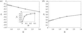
. The results for
 $J_{1}$
and
 $J_{2}$
are shown in figure 2. For
 $St\geqslant 0.7$
,
 $J_{1}$
and
 $J_{2}$
are evaluated using (2.21); for comparison, in figure 2(a) we also plot
 $J_{1}$
for
 $St\leqslant 0.3$
, which we evaluate using the
 $St\ll 1$
approximation
 $$\begin{eqnarray}\mathfrak{d}_{\Vert ,1}^{[+,-]}\approx -\frac{St\,{\it\tau}_{{\it\eta}}}{3}r\left\langle \mathscr{Z}^{p}(t,t)\right\rangle _{\mathscr{ Z}^{[+,-]}},\end{eqnarray}$$
which essentially describes the contribution from the traditional Maxey centrifuge mechanism described in the introduction (note that under the
 $St\ll 1$
approximation,
 $\mathfrak{d}_{\Vert ,2}^{[-]}=\mathfrak{d}_{\Vert ,2}^{[+]}\approx 0$
such that
 $J_{2}$
is undefined and is therefore not plotted). The results in figure 2 show that for
 $St>0$
,
 $J_{1}>-1$
and
 $J_{2}<1$
, consistent with preferential concentration. That
 $-1\leqslant J_{1}<0$
reflects the fact that the clustering mechanism associated with term
 $\unicode[STIX]{x2460}$
causes particles to drift away from
 $\mathscr{Z}^{[-]}$
regions and drift into
 $\mathscr{Z}^{[+]}$
, and is directly associated with the centrifuge mechanism acting along the particle trajectories. In contrast,
 $0\leqslant J_{2}<1$
signifying that the mechanism associated with term
 $\unicode[STIX]{x2461}$
, the non-local clustering mechanism, causes particles to drift into both
 $\mathscr{Z}^{[+]}$
and
 $\mathscr{Z}^{[-]}$
regions. However, because of the preferential sampling of the turbulence along the particle trajectories, the drift into
 $\mathscr{Z}^{[+]}$
regions is much stronger than that into
 $\mathscr{Z}^{[-]}$
regions. These results clearly demonstrate that the non-local clustering mechanism that dominates
 $St\geqslant O(1)$
particles is fundamentally different to the traditional centrifuge mechanism, yet the particles continue to drift more strongly into
 $\mathscr{Z}^{[+]}$
regions than
 $\mathscr{Z}^{[-]}$
regions, consistent with the phenomenon of preferential concentration.
Plots of (a)
 $J_{1}$
and (b)
 $J_{2}$
as a function of
 $St$
.

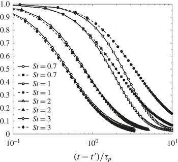
Plot of DNS data for
 ${\it\Psi}_{\mathscr{S}}$
(solid lines, open symbols) and
 ${\it\Psi}_{\mathscr{R}}$
(dashed lines, filled symbols) for various
 $St$
.

We now use the DNS data to test the key assumptions made in the theoretical analysis in § 2. First, we made the assumption that for finite
 $St$
, the Lagrangian autocorrelations of
 $\mathbf{\mathscr{S}}(\boldsymbol{x}^{p}(t),t)$
and
 $\mathbf{\mathscr{R}}(\boldsymbol{x}^{p}(t),t)$
are positive, although strictly speaking the analysis only requires that they remain positive for
 $\max [t-t^{\prime },t-t^{\prime \prime }]\leqslant O({\it\tau}_{p})$
. Figure 3 shows the autocorrelations
 $$\begin{eqnarray}\displaystyle & \displaystyle \displaystyle {\it\Psi}_{\mathscr{S}}(t,t^{\prime })\equiv \langle \mathbf{\mathscr{S}}(\boldsymbol{x}^{p}(t),t)\boldsymbol{ : }\mathbf{\mathscr{S}}(\boldsymbol{x}^{p}(t^{\prime }),t^{\prime })\rangle /\langle \mathbf{\mathscr{S}}(\boldsymbol{x}^{p}(t),t)\boldsymbol{ : }\mathbf{\mathscr{S}}(\boldsymbol{x}^{p}(t),t)\rangle , & \displaystyle\end{eqnarray}$$
 $$\begin{eqnarray}\displaystyle & \displaystyle {\it\Psi}_{\mathscr{R}}(t,t^{\prime })\equiv \langle \mathbf{\mathscr{R}}(\boldsymbol{x}^{p}(t),t)\boldsymbol{ : }\mathbf{\mathscr{R}}(\boldsymbol{x}^{p}(t^{\prime }),t^{\prime })\rangle /\langle \mathbf{\mathscr{R}}(\boldsymbol{x}^{p}(t),t)\boldsymbol{ : }\mathbf{\mathscr{R}}(\boldsymbol{x}^{p}(t),t)\rangle , & \displaystyle\end{eqnarray}$$
 $St=O(1)$
. The results clearly demonstrate that although
 ${\it\Psi}_{\mathscr{S}}(t,t^{\prime })$
and
 ${\it\Psi}_{\mathscr{R}}(t,t^{\prime })$
are affected by the particle inertia, they remain positive for
 $t-t^{\prime }/{\it\tau}_{p}\leqslant O(1)$
, confirming the assumption.
A second assumption made in our analysis was that the autocovariances
 $\langle \mathscr{Z}^{p}(t^{\prime },t^{\prime \prime })\rangle _{\mathscr{Z}^{[+,-]}}$
and
 $\langle \mathscr{Y}^{p}(t^{\prime },t^{\prime \prime })\rangle _{\mathscr{Z}^{[+,-]}}$
remain of the same sign for
 $\max [t-t^{\prime },t-t^{\prime \prime }]\leqslant O({\it\tau}_{p})$
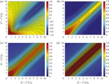
. Figure 4 plots the corresponding autocorrelations normalized by their value at
 $t^{\prime }=t^{\prime \prime }=t$
, for
 $St=1$
. The results indicate that for sufficiently large
 $t-t^{\prime },t-t^{\prime \prime }$
the autocovariances can change sign (see figure 4
a), reflecting the fact that a particle in a
 $\mathscr{Z}^{[-]}$
region at time
 $t$
, for example, may have been in a
 $\mathscr{Z}^{[+]}$
region at some earlier time in its path history. However, the results confirm that for
 $\max [t-t^{\prime },t-t^{\prime \prime }]\leqslant O({\it\tau}_{p})$
the autocovariances do not change sign, confirming the assumption in our analysis.
Contour plots of DNS data at
 $St=1$
for (a)
 $\langle \mathscr{Z}^{p}(t^{\prime },t^{\prime \prime })\rangle _{\mathscr{Z}^{[-]}}/\langle \mathscr{Z}^{p}(t,t)\rangle _{\mathscr{Z}^{[-]}}$
, (b)
 $\langle \mathscr{Z}^{p}(t^{\prime },t^{\prime \prime })\rangle _{\mathscr{Z}^{[+]}}/\langle \mathscr{Z}^{p}(t,t)\rangle _{\mathscr{Z}^{[+]}}$
, (c)
 $\langle \mathscr{Y}^{p}(t^{\prime },t^{\prime \prime })\rangle _{\mathscr{Z}^{[-]}}/\langle \mathscr{Y}^{p}(t,t)\rangle _{\mathscr{Z}^{[-]}}$
and (d)
 $\langle \mathscr{Y}^{p}(t^{\prime },t^{\prime \prime })\rangle _{\mathscr{Z}^{[+]}}/\langle \mathscr{Y}^{p}(t,t)\rangle _{\mathscr{Z}^{[+]}}$
.

A third and related assumption made in our analysis is that the time scales associated with
 $\langle \mathscr{Z}^{p}(t^{\prime },t^{\prime \prime })\rangle _{\mathscr{Z}^{[+,-]}}$
and
 $\langle \mathscr{Y}^{p}(t^{\prime },t^{\prime \prime })\rangle _{\mathscr{Z}^{[+,-]}}$
are
 ${\geqslant}O({\it\tau}_{p})$
which we estimated to be valid based on the known behaviour of
 ${\it\tau}_{\mathscr{S}}$
and
 ${\it\tau}_{\mathscr{R}}$
. The results in figure 4 show that for
 $\max [t-t^{\prime },t-t^{\prime \prime }]\leqslant O({\it\tau}_{p})$
, the autocorrelations remain significant (
 ${\gtrsim}0.5$
) demonstrating that over the memory time scale of the particle, the strain and rotation fields remain significantly correlated along the particle path history.
These results validate the key assumptions made in our analysis.
4. Conclusions
By means of theoretical analysis and tests using DNS data we have demonstrated that the non-local clustering mechanism acting in the dissipation range of turbulence with finite
 ${\it\tau}_{\mathscr{S}}$
and
 ${\it\tau}_{\mathscr{R}}$
is consistent with the phenomenon of preferential concentration. This occurs because the particles preferentially sample regions of high strain and low-rotation along their path history, and this preferential sampling affects the non-local contributions to the drift velocity generating the clustering. The
 $St=O(1)$
regime is quite distinct from the
 $St\ll 1$
regime, where preferential concentration is easily understood because the mechanism generating the clustering arises from the local preferential sampling of the fluid velocity gradient field.
For a flow with
 ${\it\tau}_{\mathscr{S}}\rightarrow 0$
and
 ${\it\tau}_{\mathscr{R}}\rightarrow 0$
, such as in the model flow field used in Gustavsson & Mehlig (Reference Gustavsson and Mehlig2011b
), or in Navier–Stokes turbulence with particles settling under strong gravity, the centrifuge mechanism no longer operates and preferential concentration vanishes. Nevertheless, inertial particles in such a system cluster because of the non-local, path history symmetry breaking mechanism.
Acknowledgements
The authors acknowledge financial support from the National Science Foundation through grant CBET-0967349 and through the Graduate Research Fellowship awarded to P.J.I. Computational simulations were performed on Yellowstone Computational and Information Systems Laboratory (2012) (ark:/85065/d7wd3xhc) at the US National Center for Atmospheric Research through its Computational and Information Systems Laboratory (sponsored by the National Science Foundation).
Appendix A. Derivation of exact RDF equation
In this appendix we outline in detail the derivation of (2.5) from (2.4). Multiplying the stationary form of (2.4) by
 $\boldsymbol{w}$
gives (written here in index notation for clarity)
 $$\begin{eqnarray}0=-w_{j}\boldsymbol{{\rm\nabla}}_{r_{i}}pw_{i}+(St\,{\it\tau}_{{\it\eta}})^{-1}w_{j}\boldsymbol{{\rm\nabla}}_{w_{i}}pw_{i}-(St\,{\it\tau}_{{\it\eta}})^{-1}w_{j}\boldsymbol{{\rm\nabla}}_{w_{i}}p\left\langle {\rm\Delta}u_{i}(\boldsymbol{r}^{p}(t),t)\right\rangle _{\boldsymbol{ r},\boldsymbol{w}}.\end{eqnarray}$$
We now integrate each term in (A 1) over all
 $\boldsymbol{w}$
 $$\begin{eqnarray}\int _{-\boldsymbol{\infty }}^{+\boldsymbol{\infty }}-w_{j}\boldsymbol{{\rm\nabla}}_{r_{i}}pw_{i}\,\text{d}\boldsymbol{w}=-\boldsymbol{{\rm\nabla}}_{r_{i}}\int _{-\boldsymbol{\infty }}^{+\boldsymbol{\infty }}pw_{j}w_{i}\,\text{d}\boldsymbol{w}=-\boldsymbol{{\rm\nabla}}_{r_{i}}{\it\varrho}S_{2,ij}^{p},\end{eqnarray}$$
 $$\begin{eqnarray}\displaystyle \int _{-\boldsymbol{\infty }}^{+\boldsymbol{\infty }}(St\,{\it\tau}_{{\it\eta}})^{-1}w_{j}\boldsymbol{{\rm\nabla}}_{w_{i}}pw_{i}\,\text{d}\boldsymbol{w} & = & \displaystyle (St\,{\it\tau}_{{\it\eta}})^{-1}\boldsymbol{{\rm\nabla}}_{w_{i}}\int _{-\boldsymbol{\infty }}^{+\boldsymbol{\infty }}pw_{i}w_{j}\,\text{d}\boldsymbol{w}-(St\,{\it\tau}_{{\it\eta}})^{-1}\int _{-\boldsymbol{\infty }}^{+\boldsymbol{\infty }}pw_{i}{\it\delta}_{ij}\,\text{d}\boldsymbol{w}\nonumber\\ \displaystyle & = & \displaystyle -(St\,{\it\tau}_{{\it\eta}})^{-1}{\it\varrho}\langle w_{j}^{p}(t)\rangle _{\boldsymbol{r}},\end{eqnarray}$$
 $$\begin{eqnarray}\displaystyle & & \displaystyle \int _{-\boldsymbol{\infty }}^{+\boldsymbol{\infty }}-(St\,{\it\tau}_{{\it\eta}})^{-1}w_{j}\boldsymbol{{\rm\nabla}}_{w_{i}}p\left\langle {\rm\Delta}u_{i}(\boldsymbol{r}^{p}(t),t)\right\rangle _{\boldsymbol{r},\boldsymbol{w}}\,\text{d}\boldsymbol{w}\nonumber\\ \displaystyle & & \displaystyle \quad =-(St\,{\it\tau}_{{\it\eta}})^{-1}\boldsymbol{{\rm\nabla}}_{w_{i}}\int _{-\boldsymbol{\infty }}^{+\boldsymbol{\infty }}pw_{j}\left\langle {\rm\Delta}u_{i}(\boldsymbol{r}^{p}(t),t)\right\rangle _{\boldsymbol{r},\boldsymbol{w}}\,\text{d}\boldsymbol{w}\nonumber\\ \displaystyle & & \displaystyle \qquad +\,(St\,{\it\tau}_{{\it\eta}})^{-1}\int _{-\boldsymbol{\infty }}^{+\boldsymbol{\infty }}{\it\delta}_{ij}p\left\langle {\rm\Delta}u_{i}(\boldsymbol{r}^{p}(t),t)\right\rangle _{\boldsymbol{r},\boldsymbol{w}}\,\text{d}\boldsymbol{w}\nonumber\\ \displaystyle & & \displaystyle \quad =(St\,{\it\tau}_{{\it\eta}})^{-1}\int _{-\boldsymbol{\infty }}^{+\boldsymbol{\infty }}\left\langle {\it\delta}(\boldsymbol{r}^{p}(t)-\boldsymbol{r}){\it\delta}(\boldsymbol{w}^{p}(t)-\boldsymbol{w}){\rm\Delta}u_{j}(\boldsymbol{r}^{p}(t),t)\right\rangle \,\text{d}\boldsymbol{w}\nonumber\\ \displaystyle & & \displaystyle \quad =(St\,{\it\tau}_{{\it\eta}})^{-1}{\it\varrho}\left\langle {\rm\Delta}u_{j}(\boldsymbol{r}^{p}(t),t)\right\rangle _{\boldsymbol{r}},\end{eqnarray}$$
where
 $$\begin{eqnarray}{\it\varrho}(\boldsymbol{r})\equiv \int _{-\boldsymbol{\infty }}^{+\boldsymbol{\infty }}p\,\text{d}\boldsymbol{w}\equiv \frac{n^{2}V}{N(N-1)}g(\boldsymbol{r}).\end{eqnarray}$$
Collecting the terms together we therefore have
 $$\begin{eqnarray}0=-\boldsymbol{{\rm\nabla}}_{r_{i}}{\it\varrho}S_{2,ij}^{p}-(St\,{\it\tau}_{{\it\eta}})^{-1}{\it\varrho}\langle w_{j}^{p}(t)\rangle _{\boldsymbol{ r}}+(St\,{\it\tau}_{{\it\eta}})^{-1}{\it\varrho}\left\langle {\rm\Delta}u_{j}(\boldsymbol{r}^{p}(t),t)\right\rangle _{\boldsymbol{ r}}.\end{eqnarray}$$
For statistically stationary, isotropic flows
 $\langle \boldsymbol{w}^{p}(t)\rangle _{\boldsymbol{r}}=\mathbf{0}$
, and so re-expressing
 ${\it\varrho}(\boldsymbol{r})$
in terms of
 $g(\boldsymbol{r})$
and multiplying (A 6) by
 $St\,{\it\tau}_{{\it\eta}}$
we finally obtain
 $$\begin{eqnarray}0=g\left\langle {\rm\Delta}u_{j}(\boldsymbol{r}^{p}(t),t)\right\rangle _{\boldsymbol{ r}}-St\,{\it\tau}_{{\it\eta}}S_{2,ij}^{p}\boldsymbol{{\rm\nabla}}_{r_{i}}g-St\,{\it\tau}_{{\it\eta}}g\boldsymbol{{\rm\nabla}}_{r_{i}}S_{2,ij}^{p}.\end{eqnarray}$$