Although research at other levels of elected office has shown that incumbency has a powerful, additive effect on votes (Hogan Reference Hogan2004; Jacobson Reference Jacobson2009; Krebs Reference Krebs1998), these effects largely have been ignored in presidential forecasting models (but see Abramowitz Reference Abramowitz2008). Instead, some scholars speculate about the conditional effects of incumbency; specifically, the decreased applicability of the retrospective model when the president is not on the ticket leaving the somewhat-harder-to-blame-or-reward vice president to represent the administration. The difficult-to-predict 2000 presidential election generated some discussion on this point. Although I and others argued (Campbell Reference Campbell2001; Holbrook Reference Holbrook2001; Wlezien Reference Wlezien2001) that part of the explanation for the forecasting error in 2000 lies with Al Gore's failure to embrace the Bill Clinton-Al Gore record and reinforce retrospective voting, others indicate that the retrospective cue may generally be weaker when the president is not on the ticket (Campbell Reference Campbell2001; Lewis-Beck and Tien Reference Lewis-Beck and Tien2001; Nadeau and Lewis-Beck Reference Nadeau and Lewis-Beck2001). Indeed, Campbell (Reference Campbell2001; Reference Campbell2008) argues in favor of only giving half weight to presidential performance variables when the vice president, rather than president, is representing the incumbent administration. The logic here is simple: absent the president on the ticket, it is more difficult to frame the election as a referendum, leading voters to attach less weight to incumbency-oriented considerations. This is not to say that factors such as presidential approval and economic performance are unimportant when incumbents do not run, only that these factors might matter less.
Rather than assuming the in-party candidate only gets half-blame (or credit) for presidential performance when the president is not running, it is better to let the data decide the appropriate weighting. As a means of assessing the importance of incumbency, I test a simple forecasting model based on my own work (Holbrook Reference Holbrook2004; Reference Holbrook2008) that controls for whether the contests involve an incumbent president. I use an index comprised of only two variables—the average rate of presidential approval and the average level of satisfaction with personal financesFootnote 1 in the summer before the presidential election—as predictors of the incumbent-party share of the two-party vote from 1952–2008, specifying that the effect of this index is stronger in incumbent than in open-seat contests.
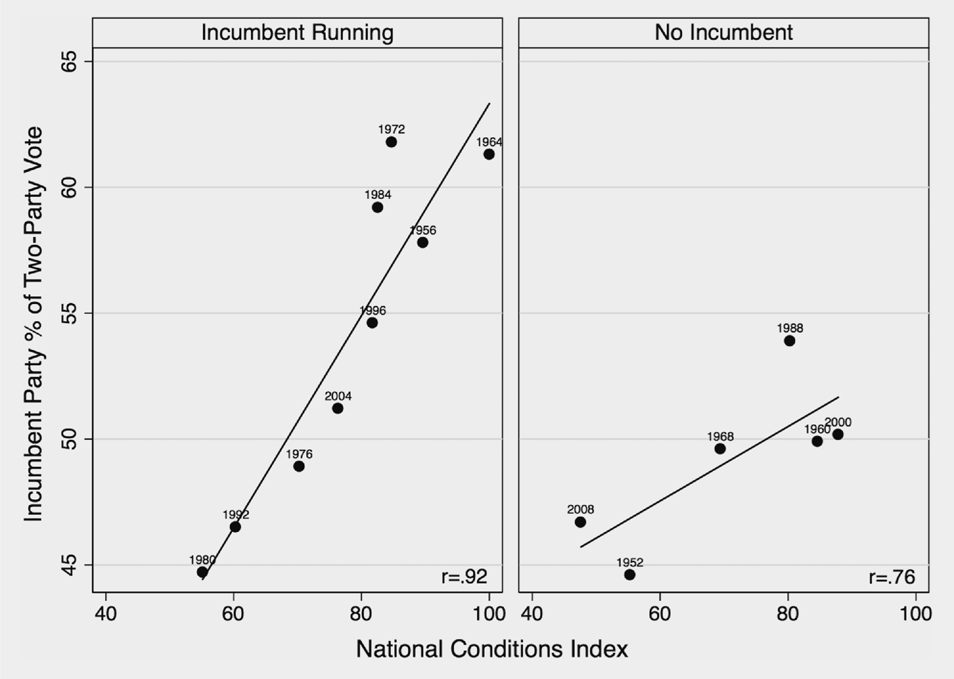
What sets this model apart is the expectation that the relationship between national conditions and presidential vote shares is weaker in nonincumbent years than in years when the incumbent is running. Indeed, for the years 1952–2008 the correlation between summer approval and incumbent party vote share is significantly stronger (.90) in years when an incumbent is running than in open-seat contests (.73); and the same pattern holds for aggregated personal finances (.88 vs. .73). Although retrospective judgments do matter in open-seat contests, as shown by the still-strong correlations, these just matter less. For the sake of parsimony, the forecasting model combines both approval and personal finances to get an overall picture of the national climate on Election Day. To do this, presidential approval and personal finances are transformed so that each observation is expressed as a percent of its highest value in the data set (both occurring in 1964): then, the two series are averaged together to provide a measure of national conditions that reflects both presidential approval and satisfaction with personal finances. The highest year on record for contests involving an incumbent was 1964 (index = 100) the lowest was 1980 (index = 55.1), and the 2012 index currently stands at 63.3. The relationship between this measure and presidential vote shares for the incumbent party is presented separately for incumbent and open-seat contest in figure 1, which illustrates the underlying point of the model: prevailing national conditions, measured during the summer before the presidential election, are closely tied to presidential election outcomes (r = .92), but that relationship is somewhat weaker during open-seat contests (r = .76).
National Conditions and US Presidential Elections, 1952–2008

THE FORECASTING MODEL
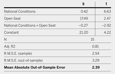
These visual patterns are summarized in more precise statistical terms in table 1, which displays the results of a regression analysis. The dependent variable in table 1 is the percent of the two-party vote going to the incumbent presidential party, and the independent variables are the measure of national conditions, which combines both approval and personal finances into a single variable, a dummy variable signifying an open-seat contest, and the interaction between national conditions and open seat contests. If there is less accountability during open-seat contests, the interaction slope should be negative and significant; indeed, table 1 indicates less accountability in years in which no incumbent is running. The impact of personal finances and presidential approval is much greater in incumbent races (b = .42) than in open-seat contests (b = .15). And despite the small sample size and high level of collinearity (tolerance = .036), the interaction term is significant at the .05 level.
Incumbency-Based Forecasting Model for US Presidential Elections, 1952–2008

Note: The dependent variable is the percent of the two-party vote won by the incumbent presidential party.
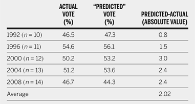
Are these findings robust, or are they due to just one or two influential data points? One way to answer this is to focus on the out-of-sample predictions, derived for each year by dropping that observation and predicting the outcome for that year based on data from the other 14 years. Doing so for this model generates an average absolute out-of-sample error of 2.39 percentage points. Another way of evaluating the expected accuracy of the model is by looking at pseudo a priori predictions from the last several elections, based on estimates that would have been (or were, in the case of 2008) generated at the time from previous elections. For instance, the predicted outcome for 1992 is based on slopes generated from data from 1952 to 1988, predictions for 1996 would be based on data from 1952 to 1992, and so on. The accuracy of these “predictions” for the last several elections is displayed in table 2. According to these estimates the model predictions for this set of elections are, on average, within just about 2 percentage points of the actual outcome.Footnote 2
Pseudo Predictions from 1992 to 2008

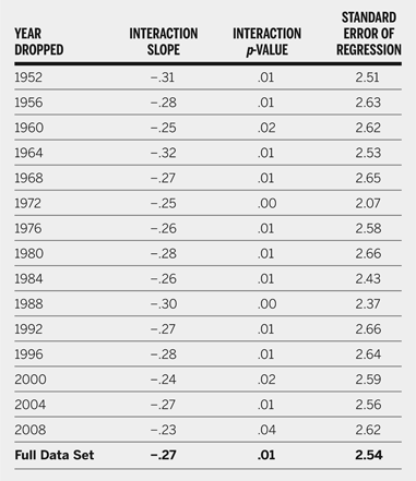
Also important, however, is whether the models overall, and the interaction term in particular, change much when single years are dropped. Table 3 provides some evidence. The entries in table 3 are the value of the interaction term, its significance level, and the root mean squared error that result when dropping each year individually from the data set. Here, we see that the magnitude and significance of the interaction slope does not change much as cases are dropped: sometimes the slope is slightly stronger, other times slightly weaker; but mostly there is little change. Although there is variation in the magnitude of the interaction slopes, the conditional role of open-seat contests does not appear to depend on the inclusion or exclusion of any single election year.
The Sensitivity of the Incumbency Interaction Term to Case Deletion

THE 2012 FORECAST
Average summer values of presidential approval (45.8%) and consumer satisfaction (86), the national conditions index stands at 63.3, which generates a preliminary predicted 2012 outcome 47.9% of the two-party vote for Barack Obama and 52.1% for Mitt Romney. This portends for a close election, especially when factoring in the small sample size and variance in predictions generated by the model. Using the (out-of-sample) standard error and the t-distribution, the estimated probability of Obama garnering more than 50% of the vote stands at .27. In terms of the standard social science treatment of significance tests, there is no significant difference between the predicted vote and an actual Obama vote of greater than 50%. At the same time, this is far less likely than a Romney vote of more than 50%. This portends a close election, but one in which Mitt Romney is the favorite.
CAVEAT
Although the model has a high level of predictive accuracy and there is every reason to expect the actual outcome will be close to the predicted outcome, there are also reasons to exercise caution. First, it is possible that one of the candidates will “Gore” the model by ignoring current conditions (Romney) or purposefully shifting attention toward other considerations (Obama). One of the assumptions I make is that both candidates understand which issues favor them, and they run the campaigns that best serve their interests. Generally, this means that the candidate favored by current conditions places them front-and-center, and the candidate who is not favored, tries to shift attention away from those issues. If both campaigns (but especially the campaign favored by conditions) are effective and strategic, voters get the referendum cue (more strongly when the president is on the ticket) and election outcomes are fairly predictable. In this way, a “campaigns matter” perspective is entirely consistent with predictable elections. Although current conditions are mixed, on balance, these favor Mitt Romney, and he should focus all of his attention on issues such as the sluggish economy. At this writing (last week in August) the Romney campaign seems to want to focus on the economy but does not seem to have figured out how to maintain that focus. In contrast, the best strategy for the Obama campaign is to shift attention from the sluggish economy. To the extent they are able to shift the focus from retrospective considerations (hence the campaign slogan, “Forward”), and toward issues that are less favorable to Romney (e.g., Bain Capital, tax returns, etc.), the outcome may reflect something other than those elements included in the model. This is clearly their strategy at this time. If either Romney's or Obama's assumed strategies dominate this fall, then the actual outcome could differ substantially from the predicted outcome.
And, of course, forecasting models have no way of incorporating significant, unexpected events—either from inside or outside the campaigns—that could significantly sway the outcome. Having said that, I am hard pressed to think of examples of such events from recent history. I assume that conventions will produce predictable bounces, in part reflecting national conditions (Holbrook Reference Holbrook1996), and that the debates will not result in much significant gains for either candidate.
CONCLUSION
The results of this analysis fit quite nicely with Campbell's (Reference Campbell2008) contention that forecasting models need to control for incumbency when using “accountability” variables. It also reflects the same sentiment found in Nadeau and Lewis-Beck's (Reference Nadeau and Lewis-Beck2001) individual-level work, which found that voters generally assigned less blame or credit to the incumbent party during open-seat contests. The upshot for the 2012 election is that as the sitting president, Obama will be held accountable for prevailing national conditions. Overall, those conditions are somewhat negative but not bad enough to heavily favor one side. Although Mitt Romney is slightly favored, the prediction generated by this model is close enough that the outcome could tip in either direction (although somewhat more likely to tip toward Romney).