1 Introduction
The majority of wind and tidal-stream turbines are of the horizontal axis type (HAWTs or HATTs). They usually operate in highly turbulent flows such as the atmospheric boundary layer and shallow tidal currents. The turbulence incident on the turbine is distorted relatively rapidly in the expanding rotor inflow, and RDT, as developed in BP and by, for example, Hunt (Reference Hunt1973) and Durbin (Reference Durbin1981), can be used to calculate the amplification of the streamwise component of the turbulent velocity as it is convected up to the plane of the rotor disc (Graham Reference Graham2017) (MG). This distortion amplifies the streamwise component of velocity sensed by the rotor and should be taken into account when carrying out predictions of unsteady loading of turbine blades using undisturbed turbulence as the input boundary condition.
The requirements for the RDT to give accurate predictions are that
 $$\begin{eqnarray}\frac{\sqrt{\overline{u_{1}^{2}}}}{\overline{U}_{1\infty }}\ll 1\quad \text{and}\quad \frac{\sqrt{\overline{u_{1}^{2}}}D}{\overline{U}_{1\infty }L_{1\infty }}\ll 1,\end{eqnarray}$$
where
 $u_{1}$
is the streamwise component of turbulent velocity,
 $\overline{U}_{1\infty }$
is the mean velocity,
 $L_{1\infty }$
is the turbulence integral length scale and
 $D$
is the diameter of the rotor. For the small length-scale result of BP to be relevant, the integral length scale of the turbulence must also be sufficiently small when compared with the rotor diameter
 $D$
for the mean velocity strain field of the rotor to be considered homogeneous locally at the eddy scale. The distortion calculations in MG were for both this case and for general turbulence length scales. The general length-scale cases required fairly extensive computation and the distortion was qualitatively similar but less than the small length-scale results.
The BP analysis gives an analytical result for small length scales, but this assumes the mean strain tensor to be diagonal, consisting of only pure compression and extension terms acting on the vorticity of the turbulence. This is a fair approximation for flow through a contracting duct, which was the original application, but not for many general flows where off-diagonal terms which rotate the vortex lines may also be important (Durbin Reference Durbin1981). In the case of a turbine inflow the effect of these terms on the streamwise turbulence amplification is small over most streamlines passing through the rotor disc, but becomes significant for streamlines passing through the tip region (
 $r(\mathit{local\,radius})/R(\mathit{tip\,radius})>0.9$
) (MG).
This RDT analysis, however, does not include the fluctuating potential flow field generated by the direct interaction of the approaching turbulence with the rotor, which is also a first-order effect. It is, therefore, not immediately applicable to comparisons with measurements of the turbulent velocities in the inflow region of a turbine. In light of this, the present paper calculates a direct fluctuating potential flow field for the rotor as an actuator disc, which is added to the distorted incident turbulence to provide estimates of the changes to the turbulent streamwise velocities occurring over the inflow region. RDT is used to calculate the streamwise turbulent velocities at general points along the axis of the inflow region. The value at the rotor plane is used as input for calculation of the fluctuating potential flow field (fluctuating pressure field) of the rotor. This result is then combined with the distortion field to provide values of turbulence intensity and spectra for the entire fluctuating velocity field at general points along the axis of the inflow region. The analyses are first computed on the basis of small length scales with the rotor as a sheet of resistance. A second computation is then carried out for turbulence of larger length scale, which is considered to be more appropriate for wind and tidal turbine rotors.
Recently, interest has focused on the changes to the intensities and spectra of the turbulent velocities in the inflow of a turbine rotor as incident turbulence is convected through this region. This is because these quantities can now be measured directly using lidar or acoustic Doppler current profiler (ADCP) instruments. To this end, the computed results are compared with published measurements taken on the upstream axis of a large-scale wind turbine in the natural turbulent wind (Peña, Mann & Dimitrov Reference Peña, Mann and Dimitrov2017) and new measurements on the upstream axis of a tidal turbine. The model is evaluated for both below-rated and above-rated turbine operational conditions.
2 Theory
2.1 Small length-scale turbulence
The action of an actuator disc on a small length-scale turbulent flow incident on the central region of the disc where the radial extent of the disc is not directly sensed is similar to that on a turbulent flow through an infinite sheet of resistance, such as a wire gauze. This is a weak turbulence, linear problem analysed by Taylor et al. (Reference Taylor, Batchelor, Dryden and Schubauer1949). The mean flow field of a horizontal axis rotor in a free stream of uniform mean velocity is represented here by the simplest axisymmetric actuator disc model (Betz Reference Betz1920). This is strictly valid only as the number of blades approaches infinity, but in practice known to be accurate, apart from very close to a blade, for small numbers of blades provided the tip speed ratio
 $\unicode[STIX]{x1D706}(=\unicode[STIX]{x1D6FA}R/\overline{U}_{\infty })\gg 1$
. Here
 $\unicode[STIX]{x1D6FA}$
is the rotation speed,
 $R$
the blade-tip radius and
 $\overline{U}_{\infty }$
the mean velocity of the free stream.
The mean velocity in the inflow region,
 $x_{1}<0$
, is given by Conway (Reference Conway1995):
 $$\begin{eqnarray}\overline{U}(r,x)=1-a\int _{0}^{\infty }\text{e}^{x_{1}x_{1}^{\prime }}\text{J}_{1}(x_{1}^{\prime })\text{J}_{0}(rx_{1}^{\prime })\,\text{d}x_{1}^{\prime },\end{eqnarray}$$
where
 $x_{1}$
and
 $x_{1}^{\prime }$
are coordinates along the axis with the actuator disc at
 $x_{1}=0$
,
 $r$
is the radial coordinate,
 $\text{J}_{0}$
and
 $\text{J}_{1}$
are Bessel functions of the first kind and
 $a$
is the wake induction factor, which depends on the rotor setting. All lengths are normalised by setting
 $R=1$
and all velocities are normalised by setting
 $\overline{U}_{\infty }=1$
. The mean axial velocity along the axis
 $r=0$
is then
 $$\begin{eqnarray}\overline{U}_{1}(0,x_{1})=1-a\left(1+\frac{x_{1}}{\sqrt{x_{1}^{2}+1}}\right)\end{eqnarray}$$
and the mean axial velocity through the actuator disc at
 $x_{1}=0$
, for all
 $r<1$
is
 $$\begin{eqnarray}\overline{U}_{1}(r,0)=1-a.\end{eqnarray}$$
The streamwise component
 $u_{1}$
of the fluctuating velocity in the inflow can be divided into a rotational part
 $u_{1r}$
and an irrotational part
 $\unicode[STIX]{x2202}\unicode[STIX]{x1D719}^{\prime }/\unicode[STIX]{x2202}x_{1}$
:
 $$\begin{eqnarray}u_{1}(r,x_{1},t)=u_{1r}+\frac{\unicode[STIX]{x2202}\unicode[STIX]{x1D719}^{\prime }}{\unicode[STIX]{x2202}x_{1}}.\end{eqnarray}$$
At the disc the potential
 $\unicode[STIX]{x1D719}$
(
 $=\unicode[STIX]{x1D719}^{\prime }$
upstream and
 $\unicode[STIX]{x1D719}^{\prime \prime }$
downstream) satisfies a pressure drop boundary condition and continuity of all fluctuating components of velocity on either side of and across the disc. Thus the only effect of this model is to generate a pressure discontinuity.
Batchelor (Reference Batchelor1953) derives the boundary condition for the
 $u_{1}$
component for an infinite gauze across a uniform turbulent flow
 $\overline{U}_{1}+u_{1}$
by linearising the pressure drop relation to get
 $$\begin{eqnarray}\left\{\frac{\unicode[STIX]{x2202}}{\unicode[STIX]{x2202}t}+\overline{U}_{1}\frac{\unicode[STIX]{x2202}}{\unicode[STIX]{x1D6FF}x_{1}}\right\}(\unicode[STIX]{x1D719}^{\prime \prime }-\unicode[STIX]{x1D719}^{\prime })=K\overline{U}_{1}\left(u_{1r}+\frac{\unicode[STIX]{x2202}\unicode[STIX]{x1D719}^{\prime }}{\unicode[STIX]{x2202}x_{1}}\right),\end{eqnarray}$$
where, in this case,
 $K=4a/(1-a)$
,
 $\overline{U}_{1}$
has to be the mean streamwise velocity at the surface of the disc because of its finite extent. Since the problem is linear, each wavenumber
 $\boldsymbol{k}=(k_{1},k_{2},k_{3})$
and frequency
 $\unicode[STIX]{x1D714}$
component of the turbulence may be considered independently. As the turbulence is assumed to be convected frozen far upstream by the mean free stream
 $k_{1}=\unicode[STIX]{x1D714}$
, the turbulence velocity there can be written as
 $$\begin{eqnarray}u_{1\infty }=\hat{u} _{1\infty }\text{e}^{\text{i}(k_{1}(t-x_{1})-k_{2}x_{2}-k_{3}x_{3})}\end{eqnarray}$$
and therefore the potential is
 $$\begin{eqnarray}\unicode[STIX]{x1D719}^{\prime }=\hat{\unicode[STIX]{x1D719}}^{\prime }\text{e}^{\unicode[STIX]{x1D70F}x_{1}}\text{e}^{\text{i}(k_{1}t-k_{2}x_{2}-k_{3}x_{3})},\end{eqnarray}$$
where
 $\unicode[STIX]{x1D70F}=\sqrt{k_{2}^{2}+k_{3}^{2}}$
, since
 $\unicode[STIX]{x1D719}^{\prime }$
satisfies
 $\unicode[STIX]{x1D6FB}^{2}\unicode[STIX]{x1D719}^{\prime }=0$
together with the condition that
 $\unicode[STIX]{x1D719}^{\prime }\rightarrow 0$
as
 $x_{1}\rightarrow -\infty$
.
The following expression can subsequently be obtained for
 $\hat{\unicode[STIX]{x1D719}}^{\prime }$
:
 $$\begin{eqnarray}\hat{\unicode[STIX]{x1D719}}^{\prime }=\frac{K(1-a)(\text{i}k_{1}-\unicode[STIX]{x1D70F})\hat{u} _{1r}(0)\text{e}^{\unicode[STIX]{x1D70F}x_{1}}}{(K+2)(1-a)\unicode[STIX]{x1D70F}^{2}+2k_{1}^{2}-\text{i}k_{1}(1-a)K\unicode[STIX]{x1D70F}}=g(\boldsymbol{k},x_{1})\text{e}^{\unicode[STIX]{x1D70F}x_{1}}\hat{u} _{1r}(0),\end{eqnarray}$$
where
 $\hat{u} _{1r}(0)$
is the amplitude of the distorted streamwise rotational component of the velocity at the actuator disc (
 $x_{1}=0$
).
The distorting effect of the mean inflow on the small length-scale turbulence is analogous to an expansion. The contraction coefficient
 $c$
, representing the expansion, is
 ${<}1$
and is related to the wake induction factor
 $a$
by
 $c=1-a$
. The streamwise component of the turbulence resulting from the distortion of the turbulent vorticity incident on the actuator disc was calculated in MG, following the BP theory, as
 $$\begin{eqnarray}\hat{u} _{1r}(0)=\frac{k^{2}\hat{u} _{1\infty }}{c(0)^{-2}k_{1}^{2}+c(0)\unicode[STIX]{x1D70F}^{2}}=f(k,0)\hat{u} _{1\infty },\end{eqnarray}$$
where
 $k^{2}=k_{1}^{2}+k_{2}^{2}+k_{3}^{2}$
and the contraction coefficient has been designated
 $c(0)$
to indicate evaluation at
 $x_{1}=0$
.
In order to calculate the whole streamwise component of the inflow turbulence at a general point
 $x_{1}\leqslant 0$
on the upstream rotor axis it is necessary to compute
 $\hat{u} _{1r}(X_{1})$
at a general point
 $x_{1}$
, where
 $X_{1}(x_{1})$
is the virtual value of
 $x_{1}$
which a fluid particle would occupy to arrive at the same time at the rotor plane
 $x_{1}=0$
if convected at the free stream velocity instead of the local mean velocity. This quantity is the Drift function discussed by Hunt (Reference Hunt1973) for non-uniform regions of mean velocity, given here in terms of an integral of the mean velocity
 $\overline{U}_{1}$
along the axis by
 $$\begin{eqnarray}X_{1}=\int _{0}^{x_{1}}\frac{\text{d}x_{1}}{\overline{U}_{1}}=\int _{0}^{x_{1}}\frac{\sqrt{x_{1}^{2}+1}\,\text{d}x_{1}}{(1-a)\sqrt{x_{1}^{2}+1}-ax_{1}}.\end{eqnarray}$$
Therefore,
 $$\begin{eqnarray}\hat{u} _{1r}(x_{1})=\frac{k^{2}\hat{u} _{1\infty }}{c(x_{1})^{-2}k_{1}^{2}+c(x_{1})\unicode[STIX]{x1D70F}^{2}}\text{e}^{-\text{i}k_{1}X_{1}}=f(\boldsymbol{k},x_{1})\text{e}^{-\text{i}k_{1}X_{1}}\hat{u} _{1\infty },\end{eqnarray}$$
noting that the function
 $f$
is real and the coefficient
 $c$
is evaluated locally at the point
 $x_{1}$
expressing the mean flow expansion from far upstream to
 $x_{1}$
.
Since the 3-dimensional spectrum tensor
 $\unicode[STIX]{x1D6F7}_{11}(\boldsymbol{k},x_{1})=\overline{\hat{u} _{1}(\boldsymbol{k},x_{1})\hat{u} _{1}^{\ast }(\boldsymbol{k},x_{1})}$
and using (2.4), (2.8) and (2.11),
 $$\begin{eqnarray}\unicode[STIX]{x1D6F7}_{11}(\boldsymbol{k},x_{1})=\{\,f^{2}+2\unicode[STIX]{x1D70F}\text{e}^{\unicode[STIX]{x1D70F}x_{1}}f(g_{R}\cos (k_{1}X_{1})-g_{I}\sin (k_{1}X_{1}))+\unicode[STIX]{x1D70F}^{2}\text{e}^{2\unicode[STIX]{x1D70F}x_{1}}gg^{\ast }\}\unicode[STIX]{x1D6F7}_{11\infty }(\boldsymbol{k}),\end{eqnarray}$$
where superscript
 $\ast$
indicates complex conjugate and
 $g=g_{R}+\text{i}g_{I}$
.
It will be assumed, as in MG, that the free stream turbulence can be considered to be approximately homogeneous and isotropic, in order to calculate specific cases, and that it may be represented approximately by the empirical von Kármán spectrum:
 $$\begin{eqnarray}\unicode[STIX]{x1D6F7}_{ij\infty }(\boldsymbol{k})=\frac{55L_{1\infty }(1.339L_{1\infty })^{2}\tilde{k}^{2}\overline{u_{1\infty }^{2}}}{9\unicode[STIX]{x03C0}(1+\tilde{k}^{2})^{17/6}}\left\{\unicode[STIX]{x1D6FF}_{ij}-\frac{\tilde{k}_{i}\tilde{k}_{j}}{\tilde{k}^{2}}\right\},\end{eqnarray}$$
where
 $$\begin{eqnarray}\tilde{k}=\frac{\unicode[STIX]{x1D6E4}(\frac{1}{3})}{\unicode[STIX]{x1D6E4}(\frac{1}{2})\unicode[STIX]{x1D6E4}(\frac{5}{6})}L_{1\infty }k=1.339L_{1\infty }k.\end{eqnarray}$$
Substituting this with
 $i=j=1$
into (2.12) the result is integrated with respect to wavenumbers
 $k_{2}$
and
 $k_{3}$
to get the frequency spectrum:
 $$\begin{eqnarray}\displaystyle & & \displaystyle \unicode[STIX]{x1D6F7}_{11}(k_{1})\nonumber\\ \displaystyle & & \displaystyle =55\iint _{0}^{\infty }\frac{\{\,f^{2}+2\unicode[STIX]{x1D70F}\text{e}^{\unicode[STIX]{x1D70F}x_{1}}f(g_{R}\cos (k_{1}X_{1})-g_{I}\sin (k_{1}X_{1}))+\unicode[STIX]{x1D70F}^{2}\text{e}^{2\unicode[STIX]{x1D70F}x_{1}}gg^{\ast }\}\tilde{\unicode[STIX]{x1D70F}}^{2}\overline{u_{1\infty }^{2}}L_{1\infty }}{9\unicode[STIX]{x03C0}(1+\tilde{k}^{2})^{17/6}}\,\text{d}\tilde{k}_{2}\,\text{d}\tilde{k}_{3}.\nonumber\\ \displaystyle & & \displaystyle\end{eqnarray}$$
The integral in (2.15) being axisymmetric may be converted to a single integral with respect to the radial wavenumber
 $\unicode[STIX]{x1D70F}$
:
 $$\begin{eqnarray}\displaystyle & & \displaystyle \unicode[STIX]{x1D6F7}_{11}(k_{1})\nonumber\\ \displaystyle & & \displaystyle \quad =110\int _{0}^{\infty }\frac{\{\,f^{2}+2\unicode[STIX]{x1D70F}\text{e}^{\unicode[STIX]{x1D70F}x_{1}}f(g_{R}\cos (k_{1}X_{1})-g_{I}\sin (k_{1}X_{1}))+\unicode[STIX]{x1D70F}^{2}\text{e}^{2\unicode[STIX]{x1D70F}x_{1}}gg^{\ast }\}\tilde{\unicode[STIX]{x1D70F}}^{3}\overline{u_{1\infty }^{2}}L_{1\infty }}{9(1+\tilde{k}^{2})^{17/6}}\,\text{d}\tilde{\unicode[STIX]{x1D70F}}.\nonumber\\ \displaystyle & & \displaystyle\end{eqnarray}$$
The intensity
 $\overline{u_{1}^{2}}(x_{1})$
may be obtained by integrating (2.16) with respect to
 $k_{1}$
. The first term (
 $f^{2}$
) in the integrand gives the result for distortion alone (as calculated in MG). The last term
 $(\unicode[STIX]{x1D70F}^{2}\text{e}^{2\unicode[STIX]{x1D70F}x_{1}}gg^{\ast })$
would give the spectrum resulting from the fluctuating potential flow field alone and the middle ‘phase’ term involving the Drift function
 $(X_{1})$
gives the cross-coupling between the two.
2.2 Application to rotors in general length-scale turbulence
In the case of general length-scale turbulence, when the small length-scale restriction is relaxed the flow must be treated as being through and round a finite diameter actuator disc. In that case, applying the unsteady form of Bernoulli’s equation upstream and downstream of the disc along the axis gives the following linearised expression for the fluctuating component of the pressure jump across the disc:
 $$\begin{eqnarray}\unicode[STIX]{x0394}p=\frac{\unicode[STIX]{x2202}(\unicode[STIX]{x1D719}^{\prime \prime }-\unicode[STIX]{x1D719}^{\prime })}{\unicode[STIX]{x2202}t}+u_{0}^{\prime }-(1-2a)u_{w}^{\prime },\end{eqnarray}$$
where
 $u_{0}^{\prime }$
is the distorted component of free stream turbulence at the disc and
 $u_{w}^{\prime }$
is a wake velocity term. This expression for
 $\unicode[STIX]{x0394}p$
can be equated to the linearised resistance expression:
 $K(1-a)(u_{\infty }^{\prime }+\unicode[STIX]{x2202}\unicode[STIX]{x1D719}^{\prime }/\unicode[STIX]{x2202}x_{1})$
. Taking the results from continuity of fluctuating velocity at the disc, as previously, to relate the downstream potential
 $\unicode[STIX]{x1D719}^{\prime \prime }$
at the disc to the upstream potential
 $\unicode[STIX]{x1D719}^{\prime }$
:
 $$\begin{eqnarray}\unicode[STIX]{x1D719}^{\prime \prime }=\frac{(1-a)^{3/2}\unicode[STIX]{x1D70F}+\text{i}k_{1}}{(1-a)^{3/2}\unicode[STIX]{x1D70F}-\text{i}k_{1}}\unicode[STIX]{x1D719}^{\prime }.\end{eqnarray}$$
This leads to an equation for the axial fluctuating potential flow velocity induced upstream on the axis:
 $$\begin{eqnarray}\frac{\unicode[STIX]{x2202}\unicode[STIX]{x1D719}^{\prime }}{\unicode[STIX]{x2202}x_{1}}=\frac{-K\unicode[STIX]{x1D70F}^{\prime }\text{e}^{\unicode[STIX]{x1D70F}^{\prime }x_{1}}u_{0}^{\prime }}{(K+4)\unicode[STIX]{x1D70F}^{\prime }+2\text{i}k_{1}/(1-a)}+\text{ a small remainder term},\end{eqnarray}$$
where
 $\unicode[STIX]{x1D70F}^{\prime }=(1-a)^{1/2}\unicode[STIX]{x1D70F}$
. This, apart from the small remainder, is half the boundary condition applied for an infinite gauze resistance. The reduction by approximately 50 % is due to the fact that this is an expanding flow only passing partly through the actuator disc. In the limit of steady flow when
 $k_{1}=0$
the equation gives the usual result for the axial component of velocity at an actuator disc.
Mann et al. (Reference Mann, Peña, Troldborg and Andersen2018) have pointed out the significance of variations of the wake induction factor
 $a$
with varying wind speeds above-rated in contrast to below-rated where it is held substantially constant. Therefore,
 $a$
can be written for above-rated wind speeds as
 $a=\overline{a}+a^{\prime }$
, where
 $\overline{a}$
is the mean value and
 $a^{\prime }=\text{d}a/\text{d}U_{\infty }u_{0}^{\prime }$
is the fluctuating component. Equation (2.18) remains unchanged except that the factor
 $(1-a)^{3/2}$
due to the distortion of the wavenumbers of the mean flow is replaced by
 $(1-\overline{a})^{3/2}$
. Then substituting in the equation for
 $\unicode[STIX]{x1D719}^{\prime }$
and linearising as before, but now also for terms in
 $a^{\prime }$
, leads to the result
 $$\begin{eqnarray}\frac{\unicode[STIX]{x2202}\unicode[STIX]{x1D719}^{\prime }}{\unicode[STIX]{x2202}x_{1}}=\frac{-\overline{K}\unicode[STIX]{x1D70F}^{\prime }\text{e}^{\unicode[STIX]{x1D70F}^{\prime }x_{1}}\left[1+(1-\overline{a}^{2}){\displaystyle \frac{\overline{U}_{\infty }}{\overline{a}}}{\displaystyle \frac{\text{d}\overline{a}}{\text{d}\overline{U}_{\infty }}}\right]u_{0}^{\prime }}{(\overline{K}+4)\unicode[STIX]{x1D70F}^{\prime }+2\text{i}k_{1}/(1-\overline{a})}+\text{ a small remainder term}.\end{eqnarray}$$
This modification to (2.19) differs only slightly from the analogous term in the quasi-steady formulation for the upstream fluctuating flow field proposed by Mann et al. (Reference Mann, Peña, Troldborg and Andersen2018):
 $$\begin{eqnarray}u_{1}^{\prime }=u_{0}^{\prime }\left[1-\overline{a}f_{s}(x)\left(1+\frac{\overline{U}_{\infty }}{\overline{a}}\frac{\text{d}\overline{a}}{\text{d}\overline{U}_{\infty }}\right)\right],\end{eqnarray}$$
where
 $-\overline{a}f_{s}(x)\overline{U}_{\infty }$
is the mean perturbation velocity field. Including the effect of varying induction factor in this way assumes that it is fully correlated with the streamwise velocity fluctuations and ignores any dynamic inflow associated with it.
3 Inflow measurements
Streamwise turbulence spectra within the inflow region of a tri-bladed HAWT with a diameter of
 $D=92.6~\text{m}$
in flat terrain were reported by Peña et al. (Reference Peña, Mann and Dimitrov2017) and Mann et al. (Reference Mann, Peña, Troldborg and Andersen2018). These were obtained from the central beam of a lidar instrument which projected horizontally from the nacelle at a hub height of 81.8 m. Results were presented for
 $x_{1}$
up to
 $-3D$
forward of the rotor, together with corresponding estimates of the axial induction factor, and encompassing both below-rated and above-rated operating conditions.
New measurements upstream of a HATT were acquired from a Nortek Signature 1000 ‘AD2CP’ which was installed on a
 $D=18.4~\text{m}$
tri-bladed rotor with a hub height of 14.5 m that operated in a mean water depth of 33 m. The general flow field, surface wave conditions and seabed characteristics in the vicinity of the HATT were reported by Coles et al. (Reference Coles, Greenwood, Vogler, Walsh and Taaff2018). The sensor was configured to measure the velocities at a rate of 4 Hz and at 0.5 m intervals between
 $x_{1}=-0.14D$
and
 $x_{1}=-1.8D$
forward of the rotor. The sensor was inclined at a relatively small inclination angle of
 $\unicode[STIX]{x1D719}=5^{\circ }$
relative to the seabed, such that the measured velocity component
 $u_{1}\cos \unicode[STIX]{x1D719}-u_{3}\sin \unicode[STIX]{x1D719}\approx u_{1}$
.
As the AD2CP measurement quality deteriorated with increasing distance from the rotor due to sensor limitations, the computation of the turbulence statistics was limited to approximately
 $x_{1}=-1.2D$
, whereas the mean velocity could be reliably estimated at greater distances upstream. The axial induction factors corresponding to the HATT were deduced from measurements of the power coefficient during the rotor operation. These were also found to be consistent with estimates from a blade element-momentum model. Velocity statistics were computed from consecutive 10 min duration samples (2400 ensembles) which overlapped by 2 min. Spectra and intensities were obtained by averaging 50 samples, for both below-rated and above-rated conditions.
4 Results and discussion
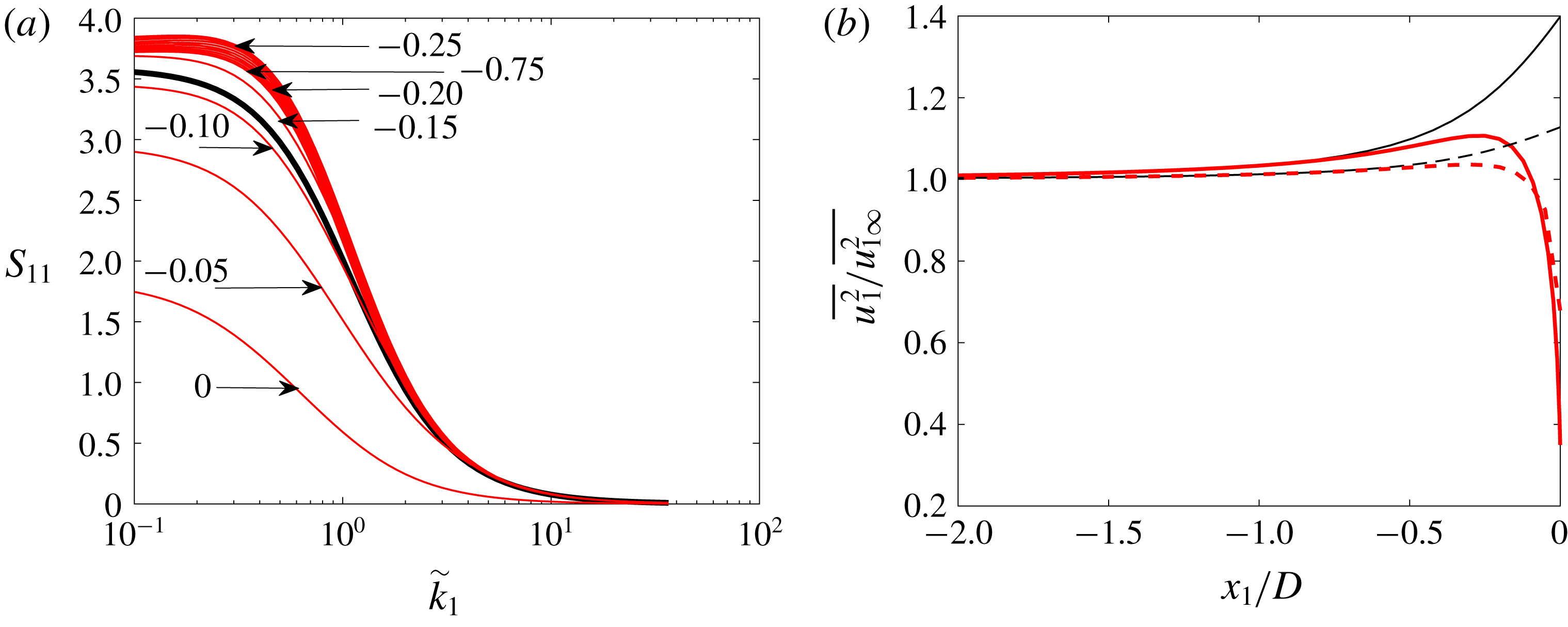
Figure 1 shows 1-dimensional frequency spectra of the streamwise component of the turbulence computed through the inflow region of a highly loaded rotor. The wake induction factor of
 $a=0.4$
corresponds approximately to the below-rated HAWT data by Peña et al. (Reference Peña, Mann and Dimitrov2017). The results are based on small length-scale theory and
 ${L_{1}}_{\infty }=0.25D$
. For both low and high frequencies the potential flow field is dominated by the distortion amplification, except close to the disc. All the distorted spectra also eventually asymptote to values very close to the undistorted spectrum at high enough frequency – except for the result at the disc itself, which remains reduced by the blocking effect for all frequencies.
(a) Spectra of streamwise turbulent velocity in the inflow region at various distances upstream of the rotor plane (
 $x_{1}/D$
labelled by arrows) for
 $a=0.4$
and
 $L_{1_{\infty }}=0.25D$
; small length-scale results. The spectra corresponding to free stream, undisturbed, conditions are shown in black. (b) Mean square intensity ratio in the inflow region for increasing upstream distance from the rotor plane, for
 $a=0.4$
(solid lines) and
 $a=0.15$
(dashed lines), with
 $L_{1_{\infty }}=0.25D$
; small length-scale results. The distortion-only results are shown in black and the total (distortion and blockage) results are shown in red.

The streamwise intensity ratios upstream of the rotor for small length scales are also plotted in figure 1. The results contrast the strong amplification due to distortion of the turbulence vorticity by the mean inflow alone with the attenuation effect when the potential flow blocking field is included. In the small length-scale limit the turbulence, away from the disc edge, is only influenced by the finite diameter of the disc through the distortion function
 $f$
, which depends on the mean inflow velocity. This function scales on the disc diameter but has also been shown in Graham (Reference Graham2017) to depend strongly on the length scale to diameter ratio of the turbulence – distortion decreasing as this ratio increases. The potential flow field (function
 $g$
) responds locally to the actuator as if it were an infinite sheet of resistance and scales on the turbulence length scale through the eddy wavenumbers. For small turbulence scales the reduction in streamwise turbulence velocity by the blocking potential flow field of the rotor greatly reduces and eventually, very close to the disc, dominates the amplification by distortion. The wake induction factor also has a significant effect on the intensities, as is demonstrated through comparisons with a lightly loaded rotor with
 $a=0.15$
, which corresponds to the HATT measurements for below-rated conditions.
The measured data are for a turbulence length scale around
 $L_{1_{\infty }}/D=1.5$
which is not small, and consideration is now given to results for larger length scales. Equation (2.19) rather than (2.5) is the boundary condition which is consistent with mean flow through an actuator disc and may therefore be regarded as more appropriate to use with large turbulence length scales and low frequencies. To that end, the calculations have been repeated using (2.19) for the boundary condition and turbulence with
 $L_{1_{\infty }}/D=1.5$
. Length scale has a strong influence on distortion. So, to avoid the extensive computations required to compute the finite length-scale distortion field at a range of points through the inflow region, the distortion flow field has been obtained from the zero length-scale results factored by the ratio of distortion for the finite length-scale
 $L_{x}=1.5D$
computed at the disc centre in Graham (Reference Graham2017) divided by the same result for zero length scale.
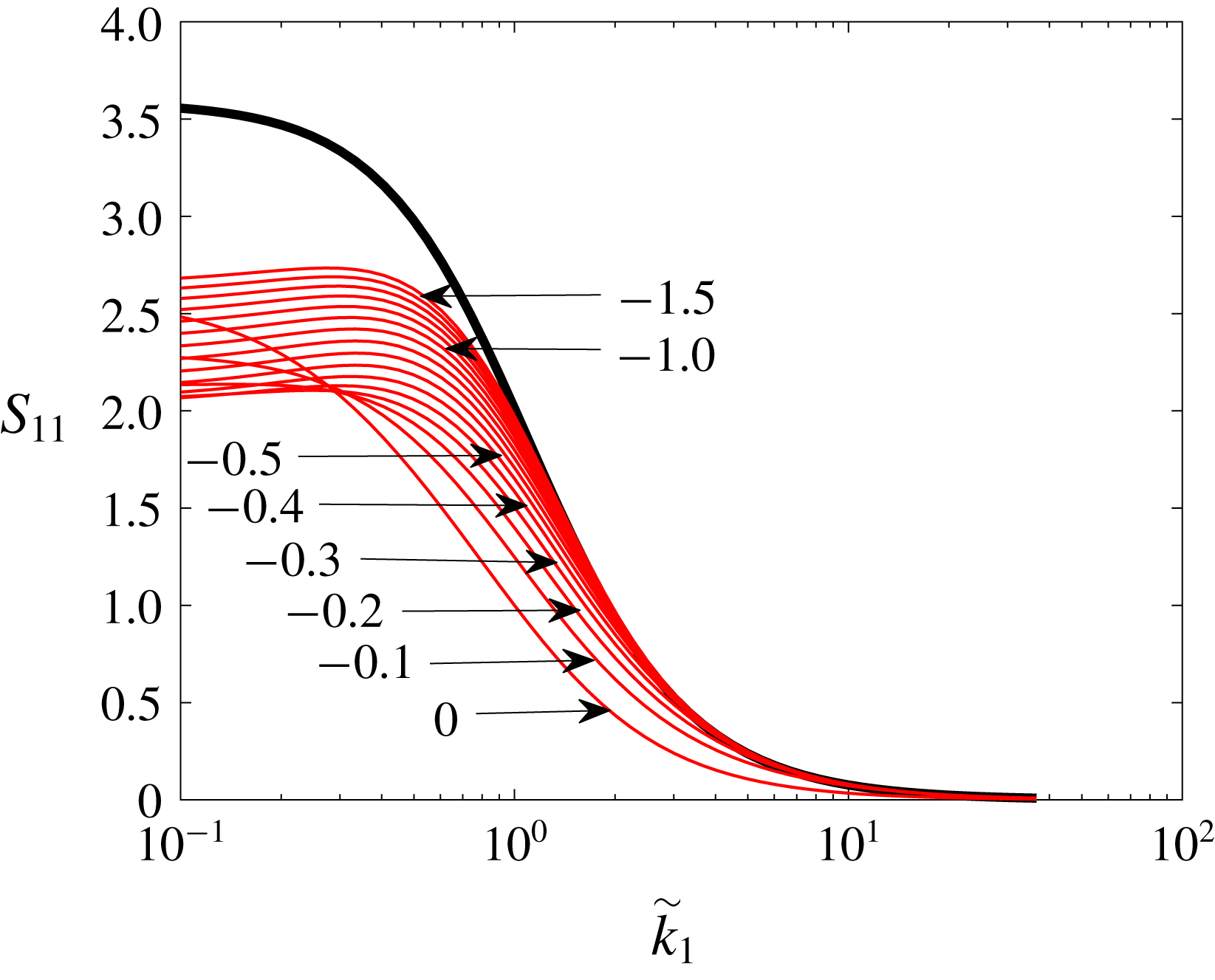
Figure 2 shows the spectra through the inflow region calculated this way for
 ${L_{1}}_{\infty }/D=1.5$
and the highly loaded (
 $a=0.4$
), below-rated rotor case. The difference due to the ‘disc’ boundary condition for the potential is evident in the low-frequency spectral components, but has very little effect on the high-frequency components. There is an attenuation of the intensities throughout the inflow region for the large length-scale case.
Spectra of streamwise turbulent velocity in the inflow region for various distances upstream of the rotor plane (
 $x_{1}/D$
labelled by arrows) for
 $a=0.4$
and
 ${L_{1}}_{\infty }=1.5D$
; larger length-scale results. The spectra corresponding to free stream, undisturbed conditions are shown in black.

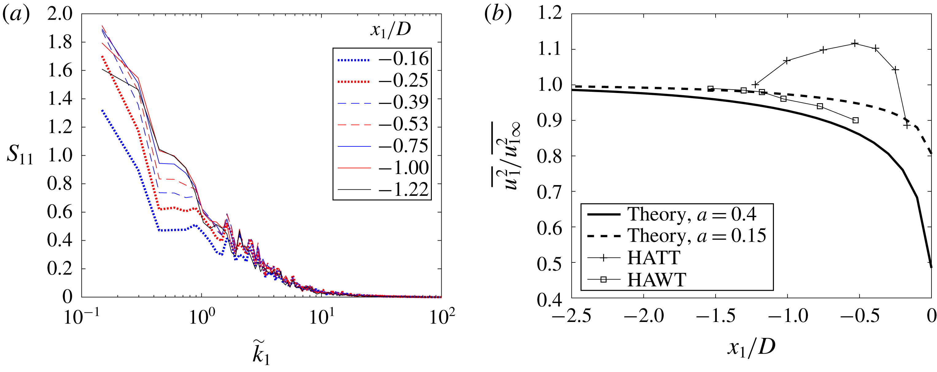
The measured spectra for the HATT for the corresponding below-rated operational conditions (i.e. with constant axial induction) are plotted in figure 3, together with theoretical intensity ratios based on the ‘disc’ boundary condition with
 ${L_{1}}_{\infty }/D=1.5$
and
 $\text{d}a/\text{d}U=0$
. The ratios of the low-frequency spectral components reported by Mann et al. (Reference Mann, Peña, Troldborg and Andersen2018), which were based on an integration of the spectral energy at low frequencies, are also presented for comparison. The attenuation of the low-frequency components for both the HATT and HAWT agrees qualitatively with the theoretical model predictions.
While the intensities were not reported by Mann et al. (Reference Mann, Peña, Troldborg and Andersen2018), the fact that the theory shows intensity attenuation, whereas the HATT results show an increase, may be due to the homogeneous actuator disc model becoming increasingly invalid at small distances upstream of the rotor. Any indication of a spectral peak at the blade passing frequency is, however, difficult to detect since this frequency was very close to the Nyquist frequency for the ADCP sampling and it might have been obscured. Additionally, there is evidence that the ratios of the transverse to the streamwise integral length scales in a marine and atmospheric bottom boundary layer (for example, Mann Reference Mann1994; Milne et al. Reference Milne, Sharma, Flay and Bickerton2013) are smaller than are assumed by the isotropic von Kármán spectrum. Since the results are highly sensitive to the transverse scales, the differences in the anisotropy may, therefore, also contribute to these differences.
(a) Streamwise spectra measured at various distances (
 $x_{1}/D$
) forward of the HATT for below-rated conditions. (b) Theoretical ratios of the intensity for
 ${L_{1}}_{\infty }=1.5D$
, compared with the measured intensity ratios for the HATT and the ratio of the low-frequency spectral components for the HAWT.

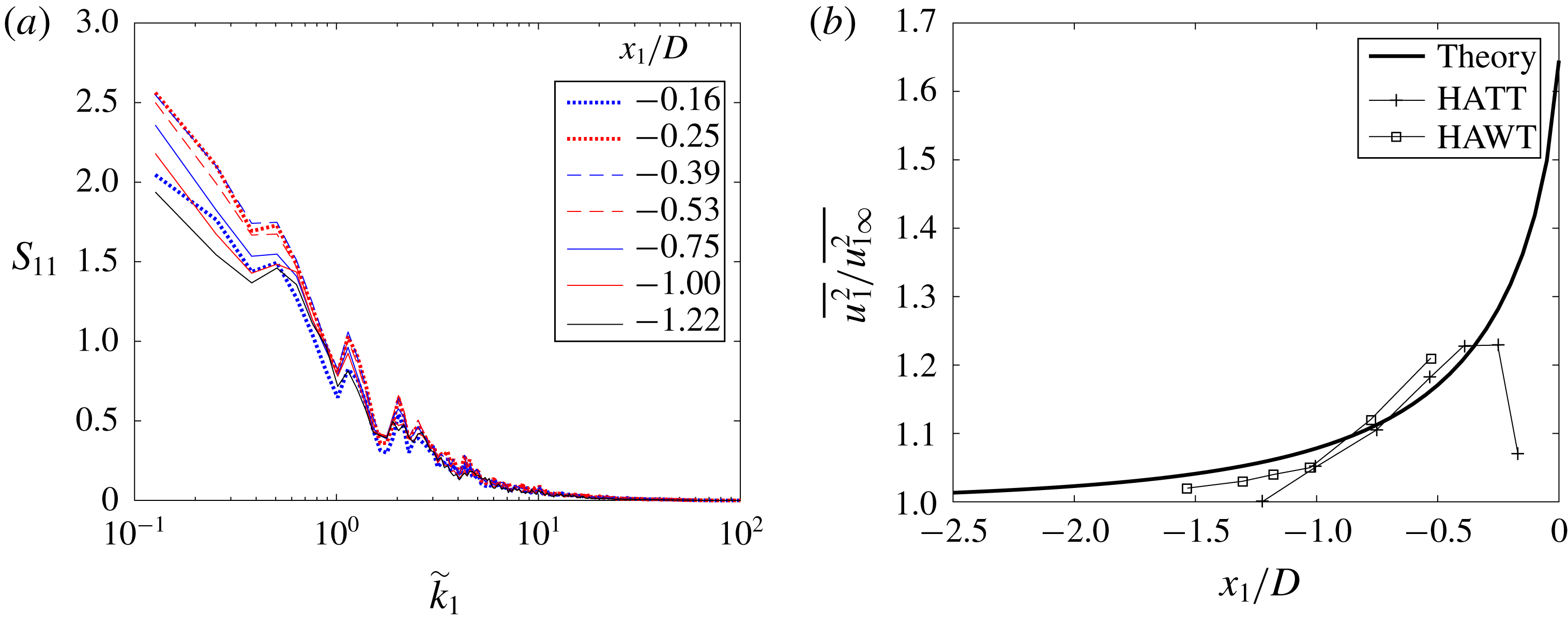
As for figure 3, for above-rated conditions, with the theoretical results corresponding to
 $\overline{a}=0.15$
,
 $(1-\overline{a}^{2})(\overline{U}_{\infty }/\overline{a})(\text{d}\overline{a}/\text{d}\overline{U}_{\infty })\approx -3.0$
.

Consideration is now made to predictions for lower loading cases where the rotor operates at above-rated power with a variable induction factor. Figure 4 shows that, in comparison to the below-rated case, the low-frequency spectral content for the HATT is amplified, except very close to the rotor. The HAWT measurements by Mann et al. (Reference Mann, Peña, Troldborg and Andersen2018) for these conditions where
 $\overline{U}_{\infty }=12~\text{m}~\text{s}^{-1}$
, indicate
 $\overline{a}\approx 0.18$
,
 $\text{d}\overline{a}/\text{d}\overline{U}_{\infty }\approx -0.05~\text{m}^{-1}~\text{s}$
, and therefore
 $(1-\overline{a}^{2})(\overline{U}_{\infty }/\overline{a})(\text{d}\overline{a}/\text{d}\overline{U}_{\infty })\approx -3.2$
. For the HATT data,
 $\overline{U}_{\infty }=3.5~\text{m}~\text{s}^{-1}$
,
 $\overline{a}\approx 0.09$
,
 $\text{d}\overline{a}/\text{d}\overline{U}_{\infty }\approx -0.08~\text{m}^{-1}~\text{s}$
, such that
 $(1-\overline{a}^{2})(\overline{U}_{\infty }/\overline{a})(\text{d}\overline{a}/\text{d}\overline{U}_{\infty })\approx -3.1$
. As these estimates are very approximate, computed results are shown in figure 4 with
 $\overline{a}=0.15$
and
 $(1-\overline{a}^{2})(\overline{U}_{\infty }/\overline{a})(\text{d}\overline{a}/\text{d}\overline{U}_{\infty })\approx -3.0$
. The results are compared with the intensity ratios measured for the HATT and the ratios of low-frequency spectral components reported by Mann et al. (Reference Mann, Peña, Troldborg and Andersen2018) for the HAWT. These results indicate that for quite typical cases the effect of the induction factor term
 $\text{d}a/\text{d}U$
(due to the time-varying rotor setting) on the fluctuating axial velocity for above-rated operation opposes the fluctuating potential blocking flow field of the rotor by as much as three times. This leads to a strong rise in this velocity ahead of the rotor which completely obscures the fall-off due to blocking. The varying induction term, which has a significant influence for above-rated operation, is not present for the results in figure 3, which are for the below-rated case. The fact that the computed results do not exhibit the final fall-off very close to the rotor plane, seen in the measured data after the strong amplification, is a failure of the simple axisymmetric actuator disc model in this region.
5 Conclusion
Rapid distortion theory has been combined with the effect of the fluctuating potential flow field to compute estimates of the intensities and spectra in the inflow of a turbine rotor. For below-rated cases the blockage opposes the distortion, resulting in an attenuation of the low-frequency spectral components. In above-rated operation the variable induction
 $a$
instead leads to an amplification of the intensities. The theoretical estimates are shown to be in qualitative agreement with measurements from both a commercial wind turbine and a tidal turbine rotor, and shows the significance of the time-varying induction factor in above-rated flows.
Acknowledgement
The provision of the HATT data by Andritz Hydro Hammerfest is greatly appreciated.