INTRODUCTION
Due to extensive land-use and land-cover change since European settlement in temperate North America, the majority of pristine wetlands have been drained, degraded, or converted to other land uses, and few sites remain free of disturbance (Cai and Yu, Reference Cai and Yu2011; Ott and Chimner, Reference Ott and Chimner2016; Byun et al., Reference Byun, Finkelstein, Cowling and Badiou2018; Loder and Finkelstein, Reference Loder and Finkelstein2020). Sediment records from remnant wetlands provide key information on wetland development, and thus have applications to wetland restoration and conservation. Temperate-zone wetlands are also under represented in estimates of soil organic carbon stocks because the more extensive and more intact boreal and sub-arctic peatlands have been a major research focus (Kolka et al., Reference Kolka, Trettin, Tang, Krauss, Bansal, Drexler, Wickland, Cavallaro, Shrestha, Birdsey, Mayes, Najjar, Reed, Romero-Lankao and Zhu2018). Net carbon uptake by temperate wetlands has been presumed to be relatively negligible or, if significant in the recent past, to be now greatly reduced by human disturbance (Armentano and Menges, Reference Armentano and Menges1986). Still, some recent studies approached estimating temperate wetland carbon stocks from national land cover, soil, or wetland inventories and attempted to estimate carbon losses at depth resulting from surface disturbances (Bridgham et al., Reference Bridgham, Megonigal, Keller, Bliss and Trettin2006; Ausseil et al., Reference Ausseil, Jamali, Clarkson and Gloubiewski2015; Nahlik and Fennessy, Reference Nahlik and Fennessy2016; Byun et al., Reference Byun, Finkelstein, Cowling and Badiou2018). Those results estimated significant carbon stocks in temperate zone wetlands, but with high uncertainties due to low densities of field measurements, particularly for wetland sediments deeper than 1 m below surface. Earlier wetland research by paleoecologists and hydrologists identified thick (>1 m) peat layers from many wetland sites in the eastern US and southern Ontario, although the carbon content was not then a major focus (e.g., Whitehead, Reference Whitehead1972; Dinel et al., Reference Dinel, Richard, Levésque and Larouche1986; Yu et al., Reference Yu, McAndrews and Siddiqi1996; Bunting and Warner, Reference Bunting and Warner1999). More recent studies have started to consider those peat observations in the context of wetland carbon sinks, and to further apply them to Holocene paleoenvironmental reconstructions (e.g., Cai and Yu, Reference Cai and Yu2011; Ott and Chimner, Reference Ott and Chimner2016; Kolka et al., Reference Kolka, Trettin, Tang, Krauss, Bansal, Drexler, Wickland, Cavallaro, Shrestha, Birdsey, Mayes, Najjar, Reed, Romero-Lankao and Zhu2018; Gutenberg et al., Reference Gutenberg, Krauss, Qu, Ahn, Hogan, Zhu and Xu2019).
In aerial views of southern Ontario (Canada), a large tract of forest cover stands out near the eastern shore of Lake Huron, in the middle of a predominantly agricultural landscape. The majority of this forest remnant is Greenock Swamp, one of the largest wetlands in the southern part of the province. This swamp escaped intensive deforestation and land use change during the early European settlement era. The surrounding areas of Bruce and Grey counties were extensively logged (Suffling et al., Reference Suffling, Evans and Perera2003). Although valuable and accessible white pines (Pinus strobus) within Greenock Swamp were targeted for timber and transported via a hand-dug canal from the late 1800s to the early 1900s, constant flooding precluded further logging within the swamp (SVCA, 1979). Later in the 20th century, the remnant swamp was recognized as a ‘provincially significant’ wetland. Previous investigations on the swamp focused on its future potential as a nature reserve and its role in watershed hydrology through shallow groundwater connections and runoff mitigation (SVCA, 1979; Johnson, Reference Johnson2000; Mansell et al., Reference Mansell, Erwin, Garraway, Howell, Jones and Harrison2004).
In most wetlands, hydrology exerts the major control on establishing the anoxic conditions needed for long-term carbon accumulation, with vegetation and climate important as well (Mitsch and Gosselink, Reference Mitsch and Gosselink2015). For a groundwater-connected wetland such as Greenock Swamp, local topography and underlying sediments promote waterlogging in conjunction with the regional groundwater balance, influenced by hydroclimate and interactions with vegetation (Brugam and Johnson, Reference Brugam and Johnson1997; Todd et al., Reference Todd, Buttle and Taylor2006; Mendyk et al., Reference Mendyk, Markiewicz, Bednarek, Świtoniak, Gamrat, Krześlak, Sykuła, Gersztyn,m and Kupniewska2016). In temperate latitudes, snowfall can also be important to support groundwater-connected wetlands (Todd et al., Reference Todd, Buttle and Taylor2006; Jiménez-Moreno et al., Reference Jiménez-Moreno, Anderson, Shuman and Yackulic2019). Postglacial hydroclimatic change is also related to wetland development via shifts in the Great Lakes water levels through the Early Holocene Lake Stanley stage and Late Holocene Nipissing rise (Magnuson et al., Reference Magnuson, Webster, Assel, Bowser, Dillon, Eato and Evans1997; Booth et al., Reference Booth, Jackson and Gray2004; Lewis et al., Reference Lewis, Blasco and Gareau2005, Reference Lewis, Heil, Hubeny, King, Moore and Rea2007; McCarthy and McAndrews, Reference McCarthy and McAndrews2012; Sonnenburg and O'Shea, Reference Sonnenburg and O'Shea2017). Paleoenvironmental analyses from this location on the leeward side of Lake Huron are relevant to addressing region-specific climate dynamics, such as the initiation and intensity of lake-effect snowfall (Henne and Hu, Reference Henne and Hu2010; Shi and Xue, Reference Shi and Xue2019), associated implications for wetland development, and the drivers of accumulation of soil carbon stocks.
The aims of this study are to (1) apply a long-core pollen record from a kettle-hole lake within the Greenock Swamp wetland complex to infer paleoclimate and vegetation history; (2) use lake and adjacent Thuja occidentalis swamp sediments to infer the timing of wetland establishment in relation to local hydrology; and (3) estimate extent of peat accumulation throughout the entire wetland basin based on topography and slope (Buffam et al., Reference Buffam, Carpenter, Yeck, Hanson and Turner2010), highlighting the potential for past, present, and future carbon sinks in this temperate swamp.
STUDY SITE AND REGIONAL SETTING
The Greenock Swamp wetland complex spans ~89 km2 within the Saugeen River watershed in the Lake Huron drainage basin (SVCA, 1979). The swamp is ~30 km away from the east shoreline of Lake Huron and is characterized by significant winter lake-effect snowfall (Fig. 1A). Before European settlement, there is evidence that a much larger wetland (>600 km2) extended beyond the current swamp area, perhaps including other natural wetlands that have now disappeared as a result of drainage and land clearing since the 1850s (Glamis Historical Researchers, Reference Kaminski2014; Byun et al., Reference Byun, Finkelstein, Cowling and Badiou2018). According to land surveyor records from the early 1800s, black ash (Fraxinus nigra) was dominant (Mansell et al., Reference Mansell, Erwin, Garraway, Howell, Jones and Harrison2004), corresponding to ‘Northern Hardwood Swamp’ described for Michigan (Kost et al., Reference Kost, Albert, Cohen, Slaughter, Schillo, Weber and Chapman2007) or ‘Floodplain Swamps’ in Low Boreal Wetland Region of Canada (National Wetlands Working Group, 1988). Now, soft maples (Acer saccharinum and A. rubrum) are dominant, and black ash (Fraxinus nigra) and American elm (Ulmus americana) are less abundant (Johnson, Reference Johnson2000), comparable to those described as ‘Southern Hardwood Swamp’ in Michigan (Kost et al., Reference Kost, Albert, Cohen, Slaughter, Schillo, Weber and Chapman2007) or ‘Hardwood treed swamp’ in the Eastern Temperate Wetland Region of Canada (National Wetlands Working Group, 1988). Thus, the current swamp tree composition is likely different from that of the pre-industrial era and seemingly reflects a northward forest range shift, which might be associated with the climate warming of recent decades (Pederson et al., Reference Pederson, D'Amato, Dyer, Foster, Goldblum, Hart and Hessl2015; Franklin et al., Reference Franklin, Serra-Diaz, Syphard and Regan2016), compounded by the effects of tree pathogens, such as Dutch Elm disease and Emerald Ash borer (Boyd et al., Reference Boyd, Freer-Smith, Gilligan and Godfray2013). Less-common trees inside the swamp include white cedar (Thuja occidentalis), which, as an understory tree, is rarely found in pure stands, tamarack (Larix laricina) in wetter areas such as the transition from a waterbody to wetland, and white pines (Pinus strobus) that attracted early settlement-era logging industry (SVCA, 1979; Johnson, Reference Johnson2000).
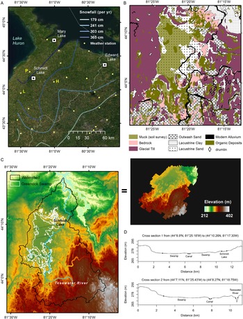
(A) Study region showing lake-effect snowfall as contours based on weather station data and locations of three lake pollen records (Table 1), including Schmidt Lake inside Greenock Swamp, Bruce County, ON. Weather station data from 1971–2000 Climate Normals (Government of Canada, https://climate.weather.gc.ca/climate\_normals/; data download 08-Jan-2020) for three stations (P: Paisley, H: Hanover, L: Lucknow) for reference modern climate values for the study site to be compared with paleoclimate reconstruction. Background satellite image credit to ESRI. (B) Close-up map of Greenock Swamp soil and substrate information (OMAFRA, undated; Ontario Geological Survey, 2010) and details in text. (C) Digital Terrain Model (DTM) map in high-resolution (2 m grid spacing) for the Teeswater River watershed and Greenock Swamp (Provincial Mapping Unit, 2015); the swamp boundary is from the provincial wetland database (Ministry of Natural Resources and Forestry, 2014) and the watershed boundary from Land Information Ontario (Open Government License—Canada). (D) Cross sections for comparison between the northern sector containing Schmidt Lake and the swamp center with Teeswater River channel. Upper cross section corresponds to upper diagonal line across Greenock Swamp in (C); lower cross section corresponds to lower diagonal line across Greenock Swamp in (C).

The hydric soil type is helpful in validating the wetland boundary, including recently drained and/or cleared areas not currently supporting wetland vegetation (Snell, Reference Snell1987). Two spatial datasets are available for Greenock Swamp soils, independent of the provincial wetland mapping (Ministry of Natural Resources and Forestry, 2014). First, the southern Ontario soil database provides a digitized map for Bruce County, showing the Greenock Swamp area dominated by the “Muck” organic soil class (Fig. 1B). This soil survey was conducted in 1948–1949 (Hoffman and Richards, Reference Hoffman and Richards1954), with organic soil chosen as the survey unit containing at least 30% organic matter by dry weight with >40 cm thickness (Ontario Ministry of Agriculture, Food and Rural Affairs, undated). The other data source is the Ontario Geological Survey (Fig. 1B), with map series published in 1986 (field work 1975–1979) for Walkerton-Kincardine area (Cowan and Pinch, Reference Cowan and Pinch1986), available in digital form (Ontario Geological Survey, 2010). This geological survey was aimed to investigate Quaternary sediments, and organic deposits were indicated only if thickness exceeded 1 m. Thus, Greenock Swamp sediments are shown in part with organic deposits thick enough (>1 m) to be mapped, but smaller than the area mapped by the soil survey (>40 cm) in Figure 1B. It is unclear how thorough the thickness measurement was for soil and surface deposits during those early surveys, and thus there is a chance that deeper organic soils are in fact present in larger areas. However, it is difficult to know how thick or dense the organic deposit was prior to anthropogenic disturbances because peat subsidence can happen quickly once drainage measures are introduced (Mirza and Irwin, Reference Mirza and Irwin1964; Leifeld et al., Reference Leifeld, Müller and Fuhrer2011; Hommeltenberg et al., Reference Hommeltenberg, Schmid, Drösler and Werle2014; He et al., Reference He, Jansson, Svensson, Björklund, Tarvainen, Klemedtsson and Kasimir2016; Sloan et al., Reference Sloan, Payne, Anderson, Gilbert, Mauquoy, Newton and Andersen2018).
The swamp organic soils are underlain by thick glaciolacustrine deposits originating from a series of proglacial lakes during the last deglaciation. According to past coastline reconstructions, there was a thin northward-elongate waterbody dammed by the Huron ice lobe to the west and the central highland of southern Ontario to the east; this waterbody lasted ~100 years (Chapman and Putnam, Reference Chapman and Putnam1984; Lewis et al., Reference Lewis, Moore, Rea, Dettman, Smith and Mayer1994) and formed the swamp's basal substrate, consisting of glacial-derived sandy deposits (SVCA, 1979; Chapman and Putnam, Reference Chapman and Putnam1984; Johnson, Reference Johnson2000), as shown in Figure 1B. This proglacial lake deposit is surrounded by thick clayey end moraine on the west side (“St. Joseph Till”), a gravelly till with a drumlin field to the south to southeast (“Elma Till”) and clayey lacustrine deposit to the north (Ontario Geological Survey, 2010). The basin topography of those glacial deposits shaped the Greenock Swamp boundary with the central flatland as mid-level elevation for the Teeswater River watershed (Fig. 1C).
The overall surface flow direction can be topographically inferred: the middle flat ground supporting the swamp is receiving runoff water from the surrounding highlands; the Teeswater River collects seasonal overflows from the swamp as well as from its upstream tributaries and flows towards the lower elevation at north (Fig. 1C). For the surface flow inside the swamp, the northern part containing Schmidt Lake is slightly higher in elevation (Fig. 1D), and the overall surface flow direction is expected towards southeast where the Teeswater River encircles. As a result, the Greenock Swamp in the watershed is effective as an intermediary water storage that mitigates overflow in downstream channels (SVCA, 1979). Before canal installation (Figs. 1D, 2), it is likely that the swamp surface water was discharged more evenly and gradually. In terms of the groundwater connection, the earlier field survey reported that the water table was <50 cm below the surface in summertime well measurements (SVCA, 1979). Although up-to-date direct measurements are lacking, a shallow groundwater depth is also estimated by a watershed potentiometric surface prediction using surrounding well records (Water Well Information System, Ontario open data; Supplementary Figure 1). The shallow groundwater can be explained by the underlying permeable sandy deposits, while the neighboring thicker clayey deposits restrict lateral discharge of groundwater (Fig. 1B; Supplementary Figure 1) (Roulet, Reference Roulet1990; McNamara et al., Reference McNamara, Siegel, Glaser and Beck1992; Todd et al., Reference Todd, Buttle and Taylor2006; Rossi et al., Reference Rossi, Ala-aho, Ronkanen and Kløve2012).
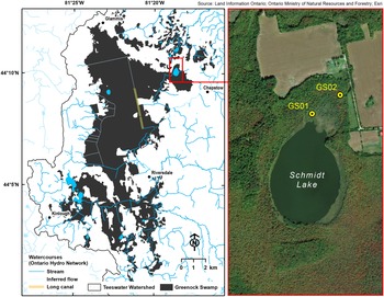
Schmidt Lake is situated in the northeast of Greenock Swamp (Fig. 2). Its round shape and the past ice sheet cover suggest that this lake is a kettle hole with ~1.5 m in maximum water depth (SVCA, 1979) (measuring point is unknown). Quaking vegetation mats of sedges and/or shrubs are found in the littoral zone. Schmidt Lake is ~3 m higher than most of the central and southern portions of Greenock Swamp (Provincial Mapping Unit, 2015), and therefore it may provide a long-term palynological record that mainly consists of wind-blown pollen from adjacent forests.
Greenock Swamp detailed map showing the surface watercourses from Ontario Hydro Network (OHN) and peat coring locations GS01 (44°10.29′N, 81°18.63′W, 281 m) and GS02 (44°10.362′N, 81°18.486′W, 283 m) in the Schmidt Lake area. Maps were created using ArcGIS software by Esri (world imagery base map in the right panel).

METHODS
Sampling and processing sediment cores
The first sediment core (GS01) for palynological analysis was taken from Schmidt Lake. Coring was performed from the quaking vegetation mat on the margin of the lake (Fig. 2), ~400 m away from the center of the lake and 10 m away from the nearest forest edge dominated by Larix laricina. In early November 2017, the quaking mat mainly supported dead cattails (Typha spp.) and sedges (Carex spp.) from the last growing season, with some wetland shrubs (e.g., Myrica gale and Chamaedaphne calyculata), and a moss layer at the surface. A serrated knife was used to collect a surface monolith of 26 cm thickness from the floating mat consisting of mosses, rhizomes, and plant roots; this monolith was stored in a sealed bag lined with plastic boards to maintain the shape during transport. Then, a Russian peat corer with a 5-cm diameter was used to collect the rest of a 725-cm-long sequence from the surface of the floating mat. The floating mat was ~50 cm thick and overlay water. The sediment-water interface was located at a depth of 150 cm from the floating mat surface. The remainder of the sequence was then collected in a series of twelve 50-cm drives from the sediment-water interface. A dense inorganic layer with angular rock particles of likely glacial origin was recorded at the base of the core. All the samples were transported to the Paleoecology lab in University of Toronto and stored in a 5°C cold room until lab analysis.
DBD (dry bulk density, g/cm3) was measured on contiguous 4-cm subsamples. The outer layer was removed from each subsample using a sharp razor blade, and the volume was measured. Subsamples were then weighed after drying in a 95°C oven for 24 hours. The dried subsamples were ground to a fine powder for measurement of total carbon (TC%) and nitrogen (TN%) contents on a LECO CN 628 analyzer (Isaac lab, University of Toronto Scarborough) and total inorganic carbon contents (IC%) by TOC-L instrument equipped with Shimadzu SSM-5000A (ANALEST, University of Toronto). The inferred total organic carbon percentages (TOC% = TC% – IC%) and organic carbon to nitrogen mass ratio (TOC/TN) were used to determine sediment types for the GS01 long core profile following the gyttja classification scheme of Łachacz et al. (Reference Łachacz, Nitkiewicz, Pisarek and Lachacz2009) and Mendyk et al. (Reference Mendyk, Markiewicz, Bednarek, Świtoniak, Gamrat, Krześlak, Sykuła, Gersztyn,m and Kupniewska2016). The core was subsampled by 1 cm3 aliquots for pollen analysis with a sampling-depth interval of 8 cm. The upper section with partial recovery of sediment (88–100 cm), between the floating mat and the deep contiguous sediment, was subsampled into 1-cm segments for pollen analysis to check if this layer includes Ambrosia pollen, indicative of the Euro-Canadian settlement zone (e.g., McAndrews, Reference McAndrews and Mahaney1981; Finkelstein and Davis, Reference Finkelstein and Davis2006; Shiller et al., Reference Shiller, Finkelstein and Cowling2014). The identification of the settlement zone within the floating mat section would support the hypothesis that settlement-era deforestation led to the formation of floating mats, as shown for other kettle-hole lakes in southern Ontario (Warner et al., Reference Warner, Kubiw and Hanf1989; Campbell et al., Reference Campbell, Duthie and Warner1997). The surface floating mat monolith was subsampled at 2-cm increments for pollen analysis. Because of lack of age control through the floating mat and difficulty obtaining precise volumetric measurements, TOC and TN analyses were not performed on the surface monolith samples.
Another sediment core (GS02) was collected in a cedar stand adjacent to the lake (Fig. 2) using the same equipment and procedure. The coring location was relatively open and wetter than areas with higher tree density dominated by Thuja occidentalis; small Larix trees were recorded at the coring location, alongside fallen and submerged logs. A 2-m-long core was collected. A woody peat layer was encountered at refusal depth; contact with underlying inorganic sediments was not reached, indicating the likelihood of a longer organic sequence. Thus, the basal peat depth at this coring location remains unknown. In this study, GS02 sediments were processed in the lab along with GS01 for C-N, DBD, and 14C age measurements but not for palynological analysis (pollen analysis was dismissed due to poor preservation and low concentration of pollen grains).
Radiocarbon ages and age-depth models
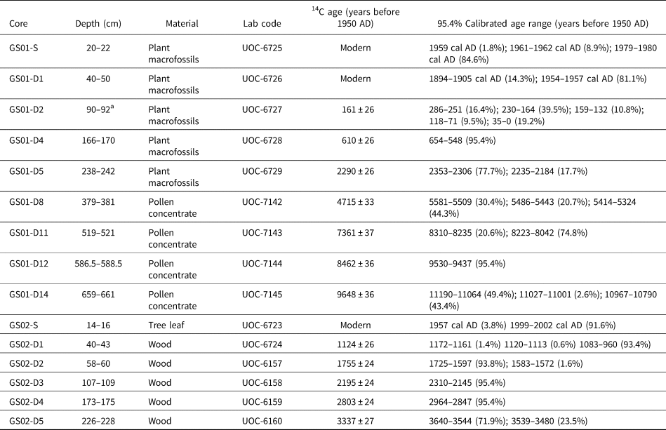
Sediment samples were examined to collect suitable materials for radiocarbon age determination. Peat samples were wet sieved (>250 μm) and scanned under a stereoscope at 40x magnification to identify terrestrial plant remains (Lévesque et al., Reference Lévesque, Dinel and Larouche1988). Wood samples from GS02 that had root hairs were avoided. For the deeper sections of GS01 with dominantly aquatic remains, such as Najas plants and mollusk shells, bulk sediment was taken and treated to extract pollen grain concentrates to obtain terrestrial carbon for dating (Brown et al., Reference Brown, Nelson, Mathewes, Vogel and Southon1989). Pollen concentrates were obtained from 8 cm3 aliquots treated with hot 10% KOH, hot 10% HCl, cold 48% HF, sieving (15–90 μm), hot 2–3% NaOCl, and placed in a clean sample tube with Milli-Q water. All these procedures were conducted in the fume hood to minimize contamination, and a radiocarbon blank and a standard sample with known concentration were processed together. A drop of final product was mounted on the microscope slide to confirm predominance of pollen grains. Five macrofossil and four pollen concentrate samples for GS01 and four wood remains for GS02 were submitted for dating to the A. E. Lalonde AMS Laboratory in Ottawa, Canada. There were no age reversals in the radiocarbon ages (Table 2).
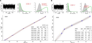
Sediment ages between the measured radiocarbon dates were inferred using Bayesian age-depth model (Blaauw and Christen, Reference Blaauw and Christen2011) in the R package “rbacon” version 2.3.9.1, with default settings for the model runs (Blaauw and Christen, Reference Blaauw and Christenundated). For GS01, pollen analysis indicated little to no Ambrosia pollen in the partial gyttja layer (88–100 cm). Thus, this section was assumed to be an originally contiguous part of the sequence below and included in the age-depth model by adjusting its position to 138–150 cm (i.e., the 50-cm water layer was omitted). Ages of the surface mat were estimated by a linear interpolation between the radiocarbon age of the sample at 20–22 cm and the sampling year for the surface (0 cm). This inference was supported by the radiocarbon result for the sample from the 40–50 cm segment (no reversal). All radiocarbon ages except those returned as modern in Table 2 were included in the Bacon model runs by their sampling depth mid-points.
Schmidt Lake pollen analysis
Eighty-two subsamples were prepared from the Schmidt Lake core GS01 for pollen analysis. The standard method for pollen sample preparation (Faegri and Iversen, Reference Faegri, Iversen, Faegri, Kaland and Krzywinski1989) was used (chemical digestions in HCl, KOH, HF, and acetolysis solution), with the addition of wet sieving to collect the 10–150 μm sized particles. Plant macrofossils were rare overall in the coarser fraction (>150 μm) of the subsample after disaggregation and sieving, but seed shells of Najas aquatic plants were identified and abundant in some depth intervals (dominant species, N. flexilis [Haynes, Reference Haynes1979; Bishop et al., Reference Bishop, Bennion, Sayer, Patmore and Yang2019]); Najas seeds were enumerated from the filtered sample remaining on the 150-μm sieve. To estimate sediment pollen concentrations, a known number of black ceramic microbeads was added to each sample at the beginning of processing (Palynotech, UK). We used a blend (SG06) with two bead sizes allowing for detection of size bias in recovery (Kitaba and Nakagawa, Reference Kitaba and Nakagawa2017). The pollen-rich pellet at the end of chemical treatment and sieving was well mixed with silicone oil, a drop of which was mounted on a glass slide for inspection at 400x (sometimes 1000x) magnification and with oil immersion for critical determinations. At least 400 grains were counted per sample. Pollen and spore identifications were made to the highest possible taxonomic resolution, following McAndrews et al. (Reference McAndrews, Berti and Norris1973) and Kapp et al. (Reference Kapp, Davis and King2000), with help of reference slides held in the Paleoecology lab, University of Toronto, and the Green Plant Herbarium (TRT) at the Royal Ontario Museum. Plant taxonomy and ecological groups (trees and shrubs, upland herbs, aquatics, and algae) followed nomenclature in the Neotoma Paleoecology Database (NeotomaDB.org) by entering the final count spreadsheet into Tilia software version 2.1.1 (by Eric C. Grimm). Pollen abundance was expressed as percent of the sum of all taxa in trees and shrubs or upland herb group (i.e., pollen sum). Fern and aquatic taxa abundance were shown as percent ratio to the pollen sum. Abundance changes of selected non-pollen palynomorphs, Pediastrum and Botryococcus, throughout the profile were estimated based on the approximate counts of cell colonies and presented as percentages of the pollen sums (thus, the counting was only valid for looking at relative abundance changes within this GS01 long core, not for absolute quantification or concentration of algal remains in sediments).
Regional pollen comparison
There are two previously published pollen records available through the Neotoma Paleoecology Database in areas adjacent to Greenock Swamp (Fig. 1, Table 1) to compare with the Schmidt Lake records. To make a pollen composite diagram for the most commonly abundant 12 tree taxa (Abies, Acer, Betula, Fagus, Fraxinus, Ostrya/Carpinus, Picea, Pinus, Quercus, Thuja, Tsuga, and Ulmus), pollen zones were newly defined using only those selected for each site record. Four pollen zones were found in common with temporal offset from radiocarbon age uncertainties (common zones, CZ 1–4). The age-depth model for Edward Lake was rerun using Bacon (Supplementary Figure 2), but larger measurement uncertainties from non-AMS radiocarbon dates and low-resolution sampling reduced robustness of the age-depth estimation. Also, the potential hard-water effect from the use of bulk sediment sample was previously corrected by assuming a regionally synchronous Tsuga decline, although this assumption has been questioned in more recent high-resolution pollen studies (e.g., Booth et al., Reference Booth, Brewer, Blaauw, Minckley and Jackson2012; Ramiadantsoa et al., Reference Ramiadantsoa, Stegner, Williams and Ives2019). The age-depth model based on AMS dating provided in Neotoma was retained for Mary Lake. In both cases we acknowledge some uncertainties in the estimated age-depth relations, given the large changes in sedimentation rates and the use of the Tsuga decline as a chronological control.
Site information for three regional pollen records.

a Ontario Hydro Network (OHN) Waterbody database archived in Ontario GeoHub (https://geohub.lio.gov.on.ca/).
b Bayesian age-depth model (Blaauw and Christen, Reference Blaauw and Christen2011) in the R package “rbacon” version 2.3.9.1 (Blaauw and Christen, Reference Blaauw and Christenundated).
c Radiocarbon (14C) ages were corrected by assuming an 800-yr reservoir effect based on assumptions about timing of Tsuga pollen decline.
d Tsuga decline (4750 ± 50 yr at 1822 cm depth from the lake surface) was included as an additional age point in the Bacon model.
Paleoclimate reconstruction
Holocene climate changes for the study site were inferred from climate-pollen relationships using the Modern Analogue Technique (MAT) (Williams and Shuman, Reference Williams and Shuman2008). A research dataset by Gonzales et al. (Reference Gonzales, Grimm, Williams and Nordheim2009) served as the modern pollen-climate reference for the MAT; this reference dataset was created from the North American Modern Pollen Database (Whitmore et al., Reference Whitmore, Gajewski, Sawada, Williams, Shuman, Bartlein and Minckley2005) by prioritizing lacustrine sites, treating erroneous sites and duplicates, performing sub-continental splits of certain taxa (Gonzales et al., Reference Gonzales, Grimm, Williams and Nordheim2009). This reference dataset was used without modification, and the taxon list of the Schmidt Lake record was adjusted for taxonomic harmonization (Supplementary Table 1). Modern analog assignments for the fossil pollen assemblages were performed using R “rioja” package version 0.9-21 (Juggins, Reference Juggins2019). Squared chord distance (SCD) was used to calculate the multivariate dissimilarity between pollen assemblages (Overpeck et al., Reference Overpeck, Webb and Prentice1985). In line with recommendations of Williams and Shuman (Reference Williams and Shuman2008), seven closest modern pollen assemblages with SCD values not exceeding 0.30 were chosen for each fossil pollen assemblage. Climate values from those modern pollen sites were averaged for plotting and presented with standard deviations of the mean values to show the spread of pollen-based climate analogs.
To address the irregular age intervals between fossil pollen samples, we compared two approaches based on the GS01 age modeling results: (1) modern pollen analogs were assigned to the fossil assemblages and then the inferred paleoclimate parameters were linearly interpolated to 100-year time steps (e.g., Viau et al., Reference Viau, Gajewski, Sawada and Fines2006); and (2) the fossil pollen data were first linearly interpolated to 100-year time steps and then the modern analogues were assigned to derive climate values (e.g., Marsicek et al., Reference Marsicek, Shuman, Brewer, Foster and Oswald2013). The first approach resulted in no analog matches for the top floating mat samples (SCD: 0.32–0.48). Because the fine scale variation among the top samples was smoothed in the second approach, all 100-year slices were found with modern assemblages within the threshold SCD 0.30 except the 5th to 7th analogs of the youngest (0 cal year BP) interpolated pollen assemblage (SCD: 0.31–0.32); this second method was used for the next step.
Paleoclimate parameters to infer from the modern pollen-analog sites were selected following the recommendation of Gonzales et al. (Reference Gonzales, Grimm, Williams and Nordheim2009). Thus, summer (June-July-August, JJA) and winter (December-January-February, DJF) monthly temperature and precipitation means were included, as well as total annual precipitation and mean annual temperature. To highlight past snowfall changes, the parameter “totsnopt” (Whitmore et al., Reference Whitmore, Gajewski, Sawada, Williams, Shuman, Bartlein and Minckley2005) was additionally chosen for the analog-based reconstruction. This annual total snowfall parameter was calculated by partitioning daily precipitation (mm per day) into snow and rain using a range of threshold temperatures (e.g., precipitation was assumed to be all snow when below -1°C; all rain when above 4°C) (P. Bartlein, personal communication, 2020). Uncertainties inherent to all pollen-based paleoclimate reconstructions are acknowledged but difficult to estimate (Birks, Reference Birks, Birks, Battarbee, Mackay and Oldfield2005). In the absence of other climate proxies, the pollen-analog results were compared to the TraCE-21ka climate model simulation for a relevant grid cell (42°30′N–45°N; 82°30′W–80°W); the representative climate values were obtained as time series using PaleoView (Fordham et al., Reference Fordham, Saltré, Haythorne, Wigley, Otto-Bliesner, Chan and Brook2017), with 100-year averaging intervals to match the time steps in the interpolated pollen time series. For reference, modern climate values for Schmidt Lake and surroundings were estimated by averaging 1971–2000 climate normal records (from the three weather stations marked in Figure 1A).
Peat volume and carbon accumulation rates
The GS02 coring and a small number of peat depth measurements at the site suggest potential significance of the Greenock Swamp peat storage. We attempted to provide an experimental estimation of the total peat stock possibly sitting in the Greenock Swamp basin. Because we had fine resolution digital terrain modeling (DTM) data for the site (Provincial Mapping Unit, 2015), a regression equation by Buffam et al. (Reference Buffam, Carpenter, Yeck, Hanson and Turner2010) derived from the positive relationship between ‘basin edge slope’ (as a predictor variable in the regression) and ‘mean peat depth’ (as a response variable) was used. We followed the procedure in ArcGIS 10.5 to calculate “ES90” (90th percentile of basin edge slope distribution) to apply it to the regression equation “Mean peat depth (m) = 0.219⋅ES90 + 0.07 (Adjusted R2 = 0.70, N = 11)” as described in (equation [3] in Buffam et al., Reference Buffam, Carpenter, Yeck, Hanson and Turner2010). The Greenock Swamp boundary follows the provincial wetland mapping within an accuracy of 200 m (Ministry of Natural Resources and Forestry, 2014). The boundary was 50-m buffered (by enlarging the Greenock Swamp polygons outbound by 50 m), and the edge layer was defined by removing the swamp boundary polygons. Slope was calculated for DTM grid cells (2 m × 2 m) inside the edge layer, and the distribution of slope values was divided into ten quantile classes to determine the 90th percentile value.
In this study, the lab analysis results from the GS01 and GS02 cores are used to give some examples of rates of carbon accumulation that took place over the Holocene. The measurements of carbon, dry bulk density, and vertical growth rates from the age-depth modeling were combined to calculate long-term apparent carbon accumulation rates (Loisel et al., Reference Loisel, Yu, Beilman, Camill, Alm, Amesbury and Anderson2014).
RESULTS
Calibrated age-depth estimations
The age-depth model from GS01 radiocarbon ages for the Schmidt Lake sequence (Fig. 3A) returned mean calendar ages BP (before present 1950 AD) ranging from 380 (178–538 cal yr BP by 95% confidence range) to 11,213 (10,914–11,576 cal yr BP) for the contiguous long sequence (155–671 cm), and from 122 (1982 AD–271 cal yr BP) to 245 (63–415 cal yr BP) for the partial gyttja segment (90–98 cm) between the water layers (see Figure 4 for coring depth profile). Samples from the uppermost floating mat returned modern radiocarbon ages from 1980 AD to the sampling year 2017 AD; therefore, an age-depth model was estimated by linear interpolation for the floating mat. The GS02 age-depth model produced calendar ages BP from 3550 (3456–3654 cal yr BP) for the oldest measurement (Fig. 3B), which we note is not the basal peat age of the coring location. The mean calendar age values computed from the Bacon model iterations (Blaauw and Christen, Reference Blaauw and Christenundated) were used to construct the y-axis of pollen diagram and to estimate rates of vertical sediment accretion in both cores.
Resulting plots from Bacon age-depth modeling for (A) the Schmidt Lake gyttja core (GS01) and (B) the woody peat core (GS02) based on radiocarbon ages in Table 2 (see the csv file input table in each panel; detailed procedure in text).

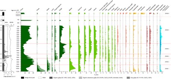
Stratigraphic sediment composition, Najas seed macrofossil counts, and percent pollen diagram for the Schmidt Lake core GS01. Pollen zones (ZONE 1–6) were determined by CONISS in the R package rioja using 82 identified taxa, but this diagram shows only the most-abundant taxa (complete dataset available at Neotoma). The y-axis was constructed based on sampling depths from the floating mat surface, including the water layer, and the tick intervals and values were determined by the calibrated radiocarbon ages from the Bacon age-depth modeling results. See text for details about gyttja sediment types.

Schmidt Lake core sediment and pollen profile
Sediment coring reached a depth of 725 cm from the floating sedge mat surface to the basal material of glacial origin. The palynologically analyzed section was dominantly organic gyttja with some variations. First, the basal ~25-cm layer consisted of coarse angular mineral grains that originated from the glacial erosion of bedrock. The overlying ~40 cm was a darker layer of fine sediment mixed with organics showing a sharp increase of TOC% towards the top, where it overlaps with the start of pollen records. Eighty-one palynomorphs were identified in the GS01 pollen record. Six zones were delineated using stratigraphically constrained cluster analysis on the 82 pollen samples (method = CONISS in the rioja R package) (Grimm, Reference Grimm1987; Bennett, Reference Bennett1996) (Fig. 4). In the estimation of pollen influx rate for individual taxa (grains cm2 yr-1), the trends and peaks across taxa are overall the same as the percentage diagram, and therefore we do not discuss influx details here (influx data are shown in Supplementary Figure 3). The pollen zonation is supplemented with a schematic showing a depth profile of sediment composition (Fig. 4).
ZONE 1 (~11,200–9600 cal yr BP)
ZONE 1 began with a decline of Picea, followed by an increase of Betula and a fluctuation of Pinus. Betula reached a maximum at ca. 10,500 cal yr BP replacing Pinus and Picea, and then declined as Pinus increased again towards the top of the zone. Abies increased with Betula and remained relatively higher than any other zone throughout the record. This zone also had high values of Larix (in consideration of its low pollen production/dispersal rate). There were small rises of Thuja/Juniperus before the peak level of Betula. Low levels (<5%) of several deciduous taxa, such as Ulmus, Fraxinus, Ostrya/Carpinus, and Carya, were already present. Among the wetland shrub taxa, Salix was abundant. Poaceae, Artemisia, and Cyperaceae recorded high percentages at the lower half of this zone, before the Betula peak. Typha latifolia rose to a small peak at the beginning of this zone; occasional grains of other aquatic pollen/spore types were also recorded, summed to a group. Not shown in Figure 4 due to low abundances throughout the record, Populus formed a small peak (2–3%) at the base. Pediastrum especially dominated at the lower part of the zone. In the sediment profile, TOC% increased high enough to be classified as organic gyttja (Łachacz et al., Reference Łachacz, Nitkiewicz, Pisarek and Lachacz2009), and Najas (likely N. flexilis) seed shells were first observed in small numbers close to the transition to ZONE 2.
ZONE 2 (~9600–8200 cal yr BP)
ZONE 2 was dominated by Pinus, approaching 60%, as Picea reached a minimum at the transition from the previous zone. Abies and Betula decreased throughout, Larix decreased to a low in the middle, and Thuja/Juniperus began low, but increased from midway towards the top. Although not differentiated, Thuja/Juniperus pollen grains were likely Thuja occidentalis (eastern white cedar), as in other parts of southern Ontario (|Yu, Reference Yu1997, Reference Yu2003). Acer and Ostrya/Carpinus rose to peak levels at ca. 8800 cal yr BP when Tsuga increased and Pinus decreased. At this horizon, Fraxinus nigra-type pollen reached a minimum, coincident with minima in Larix, while Ulmus fluctuated at low levels similar to ZONE 1. Fagus pollen was identified by only a few grains. All the herb types were recorded at low percentages compared to ZONE 1. Aquatic types were rare and less diverse than in the previous zone, shifting at the mid-point from a few grains of Typha latifolia to Potamogeton and Sphagnum towards the top. Both algal remains are relatively low. The sediment changed to organic calcareous gyttja (Łachacz et al., Reference Łachacz, Nitkiewicz, Pisarek and Lachacz2009), with lower TOC% (many mollusk shells preserved), but also had some degree of light and dark laminations.
ZONE 3 (~8200–7300 cal yr BP)
ZONE 3 had maxima of Thuja/Juniperus and Quercus, increases of Tsuga and Ulmus, and a large fluctuation of Pinus culminating in a low (<20%) at the end of this zone. Picea, Abies, Larix, and Betula remained low throughout the zone. Acer increased, and Fraxinus nigra-type recovered its abundance similar to ZONE 1. Fagus started to increase in this zone. Fraxinus americana-type and Carya attained higher percentages than the previous zones. Compared to ZONE 2, there were more shrubs (Alnus, Salix, and Rosaceae undifferentiated) and herbs (e.g., Artemisia and Cyperaceae alternate), and the algae group was dominated by Botryococcus. The sediment returned to dark organic gyttja, and Najas seed shells were most abundant with other residues of this plant.
ZONE 4 (~7300–4800 cal yr BP)
ZONE 4 had maxima of Tsuga, Fagus, and Ulmus and a minimum of Pinus. High fluctuating Tsuga was a main feature of this zone, reaching a peak at ca. 5100 cal yr BP, the highest percentage in the entire sequence. Betula increased towards the top and formed a peak coincident with low Tsuga. The algae group continued to increase, with Botryococcus still dominant. Najas seed shells briefly disappeared, but re-appeared and persisted afterwards.
ZONE 5 (~4800–120 cal yr BP)
ZONE 5 began with a sharp increase of Pinus and an abrupt decline of Tsuga at the transition from ZONE 4. Tsuga remained low (~5%), but then nearly doubled to remain until it started to increase again to another peak. Deciduous trees responded to the Pinus and Tsuga fluctuations at the base of this zone because of the percentage computation. The Tsuga decline was followed by brief rises of Betula, Quercus, Fagus, and Ulmus, thereafter they all declined as Pinus increased. All the conifers attained higher values than the previous zone. As Pinus increased towards the top, Fagus and Ulmus decreased somewhat, and then Tsuga declined after it peaks. The trends in Cyperaceae are characterized by two rises, while the other herbs consistently remained at small numbers. Algae persisted, and the dominance changed from Botryococcus to Pediastrum. Najas became null in this zone, with the sediment becoming very dark, containing the lowest TOC/TN, but more occurrence of other macrofossils (as available for the radiocarbon dating in Table 2). TOC/TN abruptly increased at the top, probably remaining high in the partial gyttja (88–100 cm; not analyzed for TOC/TN) considering the similarity in the occurrence of herbaceous plant remains (likely sedges, consistent with the rise of Cyperaceae pollen).
Radiocarbon dates from the Schmidt Lake sediment core GS01 and swamp core GS02. “S” indicates sample in surface monolith; “D” specifies the drive number for the Russian peat core sequence.

a Depth specified in Bacon age-depth model is 141 cm, assuming that this section stratigraphically was part of the underlying sediment, not the floating mat.
ZONE 6 (~1980–2004 AD)
ZONE 6 was characterized by a marked rise of Ambrosia and a decline of Pinus, marking deforestation at the time of Euro-Canadian settlement. Tsuga, Fagus, and Ulmus showed significant declines as well, but the other trees remained similar or increased. Large increases of wetland shrubs (Myrica and Rosaceae undifferentiated) and Cyperaceae likely resulted from the development of the sedge-shrub mat of Schmidt Lake, with distinctively peat-type sedimentation. Unique in this zone, Zea mays (corn) was identified with a large increase of Poaceae undifferentiated and other weedy taxa, such as Rumex, Asteraceae undifferentiated, and Amaranthaceae, also reached high levels.
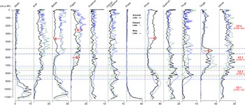
Comparison of regional pollen records
The three lake pollen records (Fig. 5) show similar trends for the important tree taxa through the Holocene (Fig. 1A; Table 1). The minimum and maximum percentages and the timing of increase (decrease) are generally coincident in most taxa, with four pollen zones in common (named CZ 1–4). Although the pollen zone transitions are asynchronous, this discrepancy could be attributed to uncertainties in age-depth modeling (Table 1). The broad similarity between the pollen records from these three regional sites lends support to the regional paleoclimate influences on vegetation development.
Comparison of percent pollen diagrams from three lake records (Fig. 1A, Table 1) for selected major tree taxa. Pollen zones were redetermined for this figure using only those selected 12 taxa by CONISS (parentheses show the original zonation of GS01 in Fig. 4). The y-axis informs the calendar age estimation of pollen samples in each core stratigraphy based on the age-depth models (Table 1 and text for details). Red arrows highlight different patterns found in the Schmidt Lake records.

Some individual taxa show some divergences among the three records, which provide insights into the role of local factors. The most pronounced discrepancy occurs in the later timing of the mid-Holocene Tsuga decline in the Schmidt Lake record. Additionally, there are local differences in abundances of tree taxa that increase following the Tsuga decline, notably Betula, Fagus, and Pinus. For example, after the Tsuga decline, there is an interval of high Pinus percentages in the Schmidt Lake instead of the rise of Betula, as in the other two lakes (CZ 4 in Fig. 5). During the interval with Tsuga maxima (CZ 3 in Fig. 5), Fagus percentages in the Schmidt Lake record are higher than in the other two lakes, but then decrease in CZ 4, also characterized by Betula and Acer in the Schmidt Lake record.
Regional climate change during the Holocene
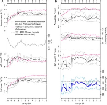
The paleoclimate reconstructions by pollen modern analogs (Fig. 6A, black lines) show long-term trends of warming from 11,200 to 8300 cal yr BP in the Early Holocene, also captured by the climate-model curves (Fig. 6A, magenta lines). In the Middle Holocene, the pollen-analog reconstructions suggest long-term cooling trends (especially summer), while the model-derived curves show continued warming in the annual and winter temperature curves. There are two parts in the Mid-to-Late Holocene cooling trends captured by the pollen analogs with peak temperatures at 4400 cal yr BP, after which both climate modeling results and pollen-based reconstructions generally reflect warming for the recent 200 years (except in the pollen-derived winter temperature). The annual total and winter monthly mean precipitations show steady increases between 9600–8300 cal yr BP, maintaining high levels since then, and the snowfall curve closely follows them (Fig. 6B). With the 1971–2000 lines as reference, the reconstructions indicate that regional climate shifted to the modern regime of warmer and wetter winters around the Mid-Holocene.
(A) Paleotemperature reconstructions from the Schmidt Lake pollen records using Modern Analogue Technique (MAT) and the climate model simulation downscaling data, and (B) precipitation reconstructions, including the pollen-based snowfall reconstructions in the lowermost panel. The pollen-based climate reconstruction curves in both panels show mean (black lines) and standard deviation (gray lines) from seven closest analog matches found in modern pollen dataset (Gonzales et al., Reference Gonzales, Grimm, Williams and Nordheim2009). Squared chord distance (SCD) was calculated repeatedly between one of the Schmidt Lake fossil pollen samples and each of the modern pollen samples until seven smallest SCD values (and thus, seven modern analog samples) were assigned for each fossil pollen (MAT). The average SCD values are plotted in the left panel below the annual mean temperature reconstruction. Horizontal lines for modern climate references (Fig. 1A and text for details).

Organic sediments and carbon accumulation rates
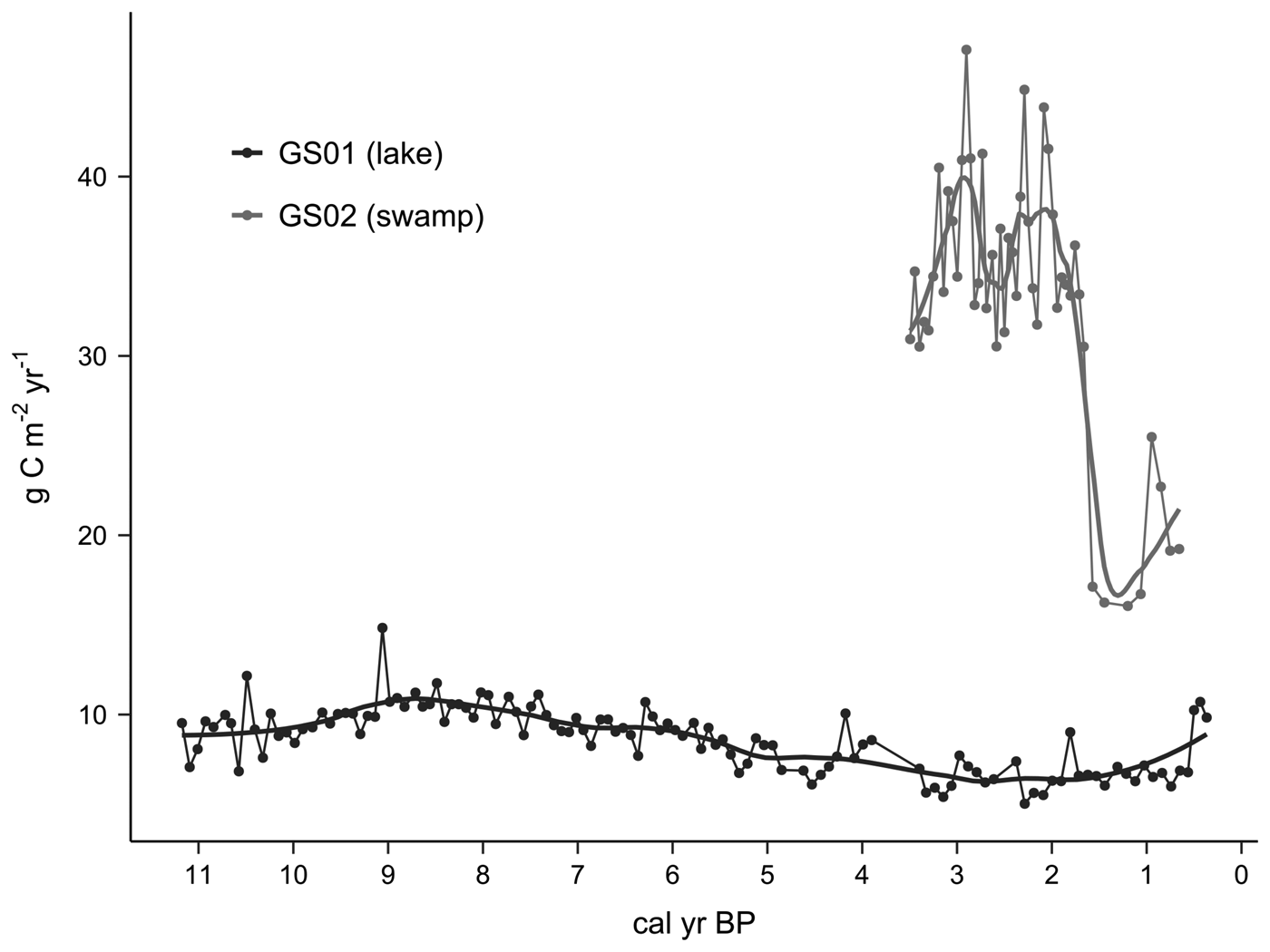
Vertical sediment accretion rates (cm/yr) were approximated using the best age-depth model curves for the gyttja layers of GS01 and the woody peat of GS02. With an average sediment accretion rate of 0.048 cm/yr, mean (± 1 SD) DBD for organic gyttja intervals (152–663 cm) of GS01 core is 0.05 ± 0.01 g/cm3, TOC content is 40.1 ± 4.89%, and mean TN content is 3.54 ± 0.53%. With a higher average sediment accretion rate of 0.079 cm/yr, mean (±1 SD) DBD for woody peat (24–224 cm) of GS02 core is 0.09 ± 0.02 g/cm3, TOC content is 49.6 ± 1.95% and mean TN content is 2.01 ± 0.46%. The changes in sediment accretion rates (cm/yr) over time were combined with depth measurement profiles of DBD (g/cm3) and TOC (%) to calculate the apparent rates of long-term carbon accumulations (g C/m2/yr) during the Holocene (Fig. 7). For the floating mat layer of the GS01 profile, a dramatic rise in the growth rate was estimated at ~0.55 cm/yr, based on the linear age-depth model.
Apparent carbon accumulation rates (g C/m2/y) with loess smoothing curves (R package ggplot; span = 0.3), based on the estimated sediment accretion rates (cm/yr) from the Bacon age-depth models, combined with changes in dry bulk density (g/cm3) and TOC (%) by depth for GS01 (dark gray; lower range) and for GS02 (gray; higher range) cores. Note that the GS02 coring did not reach the basal inorganic layer.

Average peat depth and volume of the swamp basin
The ES90 value for the Greenock Swamp basin was calculated as 9.336, and the average peat depth (2.11 m) was estimated across the swamp basin using the regression equation of Buffam et al. (Reference Buffam, Carpenter, Yeck, Hanson and Turner2010). Multiplying total swamp area (~89 km2) by this average peat depth gave the result of ~187,790,000 m3 of peat potential in the basin topography.
DISCUSSION
Holocene regional forest dynamics
Previous pollen-based research has been conducted on Holocene forest development in southern Ontario, initially showing a strong role for postglacial warming in driving the re-expansion of temperate tree species (McAndrews, Reference McAndrews and Mahaney1981). Bennett (Reference Bennett1987) suggested that species competition was the key to generating varying forest composition, even under similar climatic conditions. The general history of southern Ontario forests can be summarized as follows. The Early Holocene forests were characterized by strong boreal components, Picea (P. glauca and P. mariana) in more or less open landscape, followed by Betula (most likely B. papyrifera) and Pinus (P. banksiana and P. resinosa) increasing the overall forest density. Towards the Mid-Holocene warmer period, white pine (Pinus strobus) replaced other pines, and broadleaf trees (e.g., Acer and Ulmus) arrived. Tsuga canadensis (eastern hemlock) also migrated and played an important role in the mixed forest establishment by abrupt population changes (Fuller, Reference Fuller1998). By the Mid-Holocene, Fagus grandifolia and Acer saccharum, together with Tsuga, began to form one of the major forest associations still present today. The reoccurrence of Picea, Pinus, and Betula often characterizes the Late Holocene pollen stratigraphies of southern Ontario, suggesting the broad influence of regional cooling (Campbell and McAndrews, Reference Campbell and McAndrews1993), but locally superimposed on small-scale forest disturbances caused by indigenous Native American activities (Munoz and Gajewski, Reference Munoz and Gajewski2010).
Sub-regional white pine (Pinus strobus) forests supported within Greenock Swamp
The three pollen records (Fig. 5) were parallel until the second common zonation (CZ 2). Given that the two records have been incorporated multiple times into regional studies—Edward Lake (McAndrews, Reference McAndrews and Mahaney1981; Bennett, Reference Bennett1987, Reference Bennett1992; Fuller, Reference Fuller1997; Munoz and Gajewski, Reference Munoz and Gajewski2010) and Mary Lake (Bennett, Reference Bennett1992, Reference Bennett1993; Fuller, Reference Fuller1997)—the following discussion will focus on the divergence recorded in the new Schmidt Lake record during CZ 3 and 4 (Fig. 5) and on the aspects of relatively local forest history that appear to be different from elsewhere in the study range (i.e., the Lake Huron basin of southern Ontario). As discussed by Bennett (Reference Bennett1992), local forest composition can diverge due to each species’ unique responses to the combined effect of environmental controls and competitive interactions.
To assume that the differences recorded in the Schmidt Lake pollen represent sub-regional forest divergence, the spatial range of sub-regional forest pollen sources must be specified. Lake size is a useful parameter for predicting pollen source area (Sugita, Reference Sugita2007a, Reference Sugitab). All three lakes compared in Figure 5 are between 10–30 ha (Table 1), which is smaller than ‘large sites’ (>100 ha) where the locally sourced pollen input can be averaged, effectively presenting ‘regional’ (>104–105 km2) vegetation composition (Sugita, Reference Sugita2007a, Reference Sugitab; Hellman et al., Reference Hellman, Gaillard, Broström and Sugita2008). Thus, these three smaller lakes are more or less incorporating the local vegetation changes typically over an area of 10–100 km2 (Trondman et al., Reference Trondman, Gaillard, Sugita, Björkman, Greisman, Hultberg, Lagerås, Lindbladh and Mazier2016). The congruent patterns until CZ 2 suggest that the three local forests remained almost the same, representative of regional forest vegetation dynamics.
Thus, the divergence of Betula, Fagus, and Pinus pollen at Schmidt Lake (red arrows in Fig. 5) is likely to have resulted from adjacent forest changes, including the main body of Greenock Swamp. More Fagus in the GS01 record than the other two records during CZ 3 (Fig. 5) reflects that the pollen source area had more habitable forests for the postglacial Fagus migration from its refugial habitat in southeastern North America (Bennett, Reference Bennett1985), which may be explained by the more northerly location of the other two lakes. A more striking difference is found in CZ 4, where the Tsuga decline is followed by an increase Pinus only in the Schmidt Lake record, whereas Betula and Fagus increased at the other two sites (Figs. 4, 5). One possible explanation is the overrepresentation of Pinus pollen in littoral zone sediments due to the buoyancy of bisaccate-type grains, as recently discussed (e.g., Jones et al., Reference Jones, Williams and Jackson2017; Watson et al., Reference Watson, Williams, Russell, Jackson, Shane and Lowell2018). However, given that in CZ 1, Pinus and other bisaccate grains such as Abies and Picea are recorded at similar abundances as in the other two records where cores were retrieved from lake centers, we assume that the GS01 record had not been majorly influenced by the shoreward sorting problem. Thus, the Pinus pollen increase in CZ 4 is interpreted here as relatively more pine trees in the sub-regional forests near the Schmidt Lake, diverging from the regional trend. White pine is considered early successional on poorly developed soils, but white pine also can use disturbance gaps to establish in old forests, whereas yellow birch is late-successional and forms a mature forest with Acer, Fagus, and Tsuga (Bennett, Reference Bennett1987; Fahey et al., Reference Fahey, Lorimer and Mladenoff2012).
The glaciolacustrine and outwash deposits surrounding Schmidt Lake may be relevant in explaining the marked increase in Pinus following the Tsuga decline. Outwash plains are more susceptible to fire owing to good drainage of coarser deposits, suitable for early-successional pine establishment within a climatically habitable range of the Great Lakes region (e.g., Abrams, Reference Abrams2001; Fahey et al., Reference Fahey, Lorimer and Mladenoff2012; Fahey and Lorimer, Reference Fahey and Lorimer2014). Although the Schmidt Lake core was not inspected for fossil charcoal, the potential increase of fire frequency cannot be ruled out during CZ 4, especially with regional climate tending to be drier at the time (e.g., Booth et al., Reference Booth, Jackson and Thompson2002, Reference Booth, Jackson and Gray2004; Finkelstein and Davis, Reference Finkelstein and Davis2006; Booth et al., Reference Booth, Brewer, Blaauw, Minckley and Jackson2012). The Greenock Swamp wetland basin may have been an important source habitat for the nearby forest gaps created on the outwash deposits, given that some degree of poor drainage is advantageous for white pine seedlings to avoid competition with shade-tolerant, late-successional trees (Fahey and Lorimer, Reference Fahey and Lorimer2014). Under this hypothesis, white pine populations would have quickly established in canopy gaps due to nearby seed sources and habitat-disturbance relationships in the Schmidt Lake sub-region. Meanwhile, competitive interactions by Betula and Acer within the same old-forest stands were filling the gaps produced by the Tsuga decline at the other two nearby lake sites (McAndrews, Reference McAndrews and Mahaney1981; Bennett, Reference Bennett1992).
As Tsuga started to regain some dominance, the white pine trees persisted benefiting from the Late Holocene cooling, peaking in the Little Ice Age (ca. 500 cal yr BP), which again interrupted Tsuga expansion across the study region and most of southern Ontario (e.g., Campbell and McAndrews, Reference Campbell and McAndrews1993; Yu et al., Reference Yu, McAndrews and Siddiqi1996; Finkelstein and Davis, Reference Finkelstein and Davis2006). The European settlement logging industry probably exploited the white pines established during the Little Ice Age. The observed sharp decline of Pinus after this time (Fig. 4) indicates the initial success of logging on the upland forests, later expanding to the large Greenock Swamp white pines growing in the marginal habitats along the Teeswater River channels. Before logging, the main body of Greenock Swamp was dominated by Fraxinus nigra, as mentioned in the early land survey (Mansell et al., Reference Mansell, Erwin, Garraway, Howell, Jones and Harrison2004), with more Ulmus than recorded in modern observations (Johnson, Reference Johnson2000); these observations are also supported by the pollen profile (the top of ZONE 5 in Figure 4). At this time, the Schmidt Lake area was likely similar to what would currently be considered “mixed” swamp: hardwoods intermixed with Thuja swamps that were accumulating peat, scattered Larix, and sedge-dominated marshes on the wetter side close to the open water.
The high Pinus percentages at Schmidt Lake during the Late Holocene is partly an artefact due to the importance of non-prolific pollen producers (Fraxinus, Ulmus, Larix, and Thuja) in the temperate swamp communities (Sugita et al., Reference Sugita, Parshall and Calcote2006; Kujawa et al., Reference Kujawa, Goring, Dawson, Calcote, Grimm, Hotchkiss and Jackson2016) than to a regionally widespread cover of pine forests like the Early Holocene. It has been recognized as a myth that southern Ontario forests were once greatly populated by large white pine trees before the European settlement (the observation was likely biased during the early surveys and reports pursuing most resourceful stands; Suffling et al., Reference Suffling, Evans and Perera2003). We suggest that Greenock Swamp and surrounding area actually had quite a number of local to sub-regional white pine stands, benefiting from the combination of outwash deposits and abundant marginal habitats for persistent seed sources (Fahey and Lorimer, Reference Fahey and Lorimer2014). However, large-scale deforestation and wetland conversion in southern Ontario make it difficult to observe ecological aspects of white pine in the wet forest domain (Abrams, Reference Abrams2001; Suffling et al., Reference Suffling, Evans and Perera2003; Fahey et al., Reference Fahey, Lorimer and Mladenoff2012; Fahey and Lorimer, Reference Fahey and Lorimer2014).
Potential expansion of hardwood lowland forests
Lake pollen records are often used to reconstruct forest dynamics focusing on upland habitats where the majority of pollen source trees were assumed to grow. This study suggests that the past significance of lowland forests has been underestimated in Holocene forest history of southern Ontario, as well as the significance of naturally abundant wetland habitats. Revisiting pollen records in consideration of regionally representative swamp taxa can give some insight into past wetland expansion. For example, Ulmus shows similar change in the three lake pollen records (Fig. 4), and its increases from the time of CZ 2 (Fig. 5; since ca. 8300 cal yr BP, following the Schmidt Lake pollen zonation) might have resulted from expansion of elm-dominant hardwood swamp into the study region. According to one of the few direct observations of extensive and abundant swamp forests existing prior to land clearance during the era of European settlement (Sampson, Reference Sampson1930), the primary swamp community was “elm-black ash-soft maple” forest with American elm (Ulmus americana), black ash (Fraxinus nigra), and soft maples (Acer rubrum and A. saccharinum), which can tolerate the initial wettest conditions and then may incorporate less-tolerant species while Ulmus remains dominant. In pollen-inferred forest cover reconstructions, flood-tolerant trees can be underrepresented due to their low to moderate pollen productivity and dispersal range (Webb et al., Reference Webb, Cushing, Wright and Wright1983; Dawson et al., Reference Dawson, Paciorek, McLachlan, Goring, Williams and Jackson2016; Kujawa et al., Reference Kujawa, Goring, Dawson, Calcote, Grimm, Hotchkiss and Jackson2016). Therefore, the consistent Ulmus rises across the three sites (Fig. 5) may indicate a region-wide development of elm swamp communities while Tsuga was increasingly forming mesic forest communities in the uplands. Together, these trends indicate that the landscape was getting wetter overall (Brugam and Johnson, Reference Brugam and Johnson1997). Even without the major settlement-era wetland losses, it would be difficult to find a modern example of extensive Ulmus (hardwood swamp) forest in North America due to the spread of Dutch Elm disease (Marks, Reference Marks, Pinchot, Knight, Haugen, Flower and Slavicek2017). Fraxinus is also undergoing decline due to the expansion of Emerald Ash borer (Van Grinsven et al., Reference Van Grinsven, Shannon and Bolton2018).
Questioning the assumption of synchronous Tsuga decline
We highlight the need for future studies on the Mid-to-Late Holocene Tsuga decline. The percentage changes in Tsuga are comparable among the three records, but the timing of decline clearly differs (CZ 3–4 in Figure 5). The radiocarbon age calibration of the Schmidt Lake record (GS01) revealed that a ‘final’ Tsuga decline that occurred between 4951 (4540–5275) and 4773 (4337–5143) cal yr BP, determined by a decline by more than half in percentage values. This timing is later than the previously estimated synchronous decline at 4800 or 4750 14C yr BP (ca. 5450 cal yr BP) (Bennett and Fuller, Reference Bennett and Fuller2002; Booth et al., Reference Booth, Brewer, Blaauw, Minckley and Jackson2012) that was used as a chronological marker for the other two pollen sites. This observation supports the notion of an asynchronous decline of Tsuga across eastern North America (Booth et al., Reference Booth, Brewer, Blaauw, Minckley and Jackson2012). The Schmidt Lake also records pre-decline fluctuations, and the timing of the final decline corresponds to the suggestion of Booth et al. (Reference Booth, Brewer, Blaauw, Minckley and Jackson2012). The use of Tsuga decline as an age control in earlier pollen records needs to be reconsidered, not only for robust chronology but also for better understanding of forest ecology (e.g., Calcote, Reference Calcote2003; Ramiadantsoa et al., Reference Ramiadantsoa, Stegner, Williams and Ives2019).
Holocene regional climate dynamics
Pollen analog-inferred paleotemperatures (Fig. 6A) generally follow what has been found for continental-scale Holocene climate change: Early Holocene warming, the Mid-Holocene warm interval, and a Late Holocene cooling trend (e.g., Viau et al., Reference Viau, Gajewski, Sawada and Fines2006; Shuman and Marsicek, Reference Shuman and Marsicek2016; Marsicek et al., Reference Marsicek, Shuman, Bartlein, Shafer and Brewer2018). An unexpected peak at 10,800 cal yr BP may be associated with high pollen dissimilarity (high SCD values; Fig. 6A bottom) and weak representation in the climate space of modern pollen sites. For comparison, global transient climate simulations using a fully coupled CCSM3 for the last 22,000 years (TraCE-21ka project) provide paleoclimate overviews for time slices throughout the Holocene. The sudden summer temperature drop at 8200 cal yr BP (Fig. 6A) reflects collapse of the Laurentide Ice Sheet (e.g., Yu and Wright, Reference Yu and Wright2001; Shuman et al., Reference Shuman, Bartlein, Logar, Newby and Webb2002).
This study focuses on using the pollen-derived precipitation curves to describe trends over time. The absolute precipitation values may not be reliable because the entire ranges of winter and annual precipitations remain far lower than the weather station data (Fig. 6B). According to Canadian Climate Normal calculation for the three weather stations (Fig. 1A), 100 cm snow is equal to 100 mm precipitation in a monthly total calculation, regardless of the falling-snow temperature. This calculation was likely different in the pollen climate reference dataset (Whitmore et al., Reference Whitmore, Gajewski, Sawada, Williams, Shuman, Bartlein and Minckley2005; Gonzales et al., Reference Gonzales, Grimm, Williams and Nordheim2009) based on compilation of miscellaneous climate station data (New et al., Reference New, Lister, Hulme and Makin2002) (i.e., the 100 cm snow was considered <100 mm precipitation depending on the temperature range when added to monthly precipitation; see Methods for details). Thus, we mainly discuss the general patterns of reconstructed snowfall derived from pollen analogs, not the absolute values.
Onset of the lake-effect snowfall
In the Early Holocene, Lake Huron (as Lake Stanley stage) had extremely low water levels that lasted from 11,300 to 8400 cal yr BP (Lewis et al., Reference Lewis, Heil, Hubeny, King, Moore and Rea2007; Sonnenburg and O'Shea, Reference Sonnenburg and O'Shea2017), influenced by widespread drought across the upper Great Lakes region (Lewis et al., Reference Lewis, Moore, Rea, Dettman, Smith and Mayer1994, Reference Lewis, Blasco and Gareau2005; McCarthy and McAndrews, Reference McCarthy and McAndrews2012). According to the pollen-based climate reconstruction, the temperature seasonality remained high during this low lake interval, when the annual mean temperature was rising fast (Fig. 6 and Supplementary Fig. 4). Temperature changes during the Early Holocene are generally attributed to seasonal insolation patterns (Williams and Jackson, Reference Williams and Jackson2007), while the role of much-reduced lake surface cannot be ruled out for the evolution of region-specific climate controls (Scott and Huff, Reference Scott and Huff1996). The pollen-derived temperature seasonality (Supplementary Fig. 4) shows an abrupt downward shift by the end of this Lake Huron low stage. This implies that it is the subsequent recovery of lake level that starts to play a role in establishing the lake-effect climate observed today (Scott and Huff, Reference Scott and Huff1996). The climate model-derived curve only reflects the gradual decline of insolation seasonality (Williams and Jackson, Reference Williams and Jackson2007).
Recovery of Lake Huron water level and its increase in surface size may have facilitated the start of lake-effect snow, as observed today (Fig. 1A). Previous research on the northern part of lower Michigan has shown that the present lake-effect snowbelt along the leeward shoreline of Lake Michigan has been effective since 9500 cal yr BP expanding until 5500 cal yr BP (Henne and Hu, Reference Henne and Hu2010). It has been suggested that the development of a lake-effect snowbelt has strong implications for regional forest ecosystems, for example as shown by the expansion of Fagus grandifolia (Wang et al., Reference Wang, Gill, Marsicek, Dierking, Shuman and Williams2016). Our Schmidt Lake pollen record shows an increase of Fagus from ZONE 3 (Fig. 4), which supports this idea of the onset of Holocene lake-effect snowfall resulting in expanded mesic habitats suitable for ash-elm lowland forests (Wang et al., Reference Wang, Gill, Marsicek, Dierking, Shuman and Williams2016). The effective timing based on our snowfall reconstruction is ca. 8300 cal yr BP (Fig. 6), within the time range of the effect in adjacent Lake Michigan (Henne and Hu, Reference Henne and Hu2010; Wang et al., Reference Wang, Gill, Marsicek, Dierking, Shuman and Williams2016). The Mid-Holocene onset of the lake-effect hydroclimate is congruent with the downward shift of pollen-reconstructed summer precipitation as well (Scott and Huff, Reference Scott and Huff1996).
This study aimed to explore the developmental history of Greenock Swamp wetland, and the results suggest an important role for lake-effect snowfall as a region-specific climate factor. Winter precipitation is more effective for recharging regional groundwater reservoir compared to the same amount of increase during summer because some of the summer rainfall is lost to evapotranspiration (Jiménez-Moreno et al., Reference Jiménez-Moreno, Anderson, Shuman and Yackulic2019). Thus, the start of significant winter snowfall may have decreased the groundwater depth under the Greenock Swamp lowland through more recharge for the Teeswater River watershed, which persists today. The pollen-based reconstruction (Fig. 6B) shows a noticeable decrease in the annual total precipitation from 4800 to 3200 cal yr BP, which is mirrored in the decrease of mesic forest taxa such as Tsuga, Fagus, and Betula (B. alleghaniensis [Bennett, Reference Bennett1992; Booth et al., Reference Booth, Jackson and Thompson2002]) in the pollen profile (Fig. 4), and may reflect Mid-to-Late Holocene drought events recorded in other records from the Great Lakes region (e.g., Booth et al., Reference Booth, Jackson and Thompson2002, Reference Booth, Jackson and Gray2004, Reference Booth, Brewer, Blaauw, Minckley and Jackson2012; Finkelstein and Davis, Reference Finkelstein and Davis2006).
Formation of the Greenock Swamp wetland
We assume that the increased groundwater inputs in the watershed supported wetland development across the study site. Formerly part of a proglacial lake, the Greenock Swamp basin might have dried up during the Early Holocene, but saturated soils soon re-established with the onset of lake-effect snow. The local origin of green algae and Najas seed remains suggests that Schmidt Lake has maintained open water despite the organic sediment buildup and potential for terrestrialization. Given the swamp basin topography and inferred direction of water flow (Fig. 1), the main part of the swamp remained susceptible to flooding during the whole period of sediment accumulation in Schmidt Lake (Fig. 1).
Swamp paleohydrology
Schmidt Lake was likely formed in the Early Holocene when the ice block occupying the kettle-hole fully melted, like many other kettle lakes in southern Ontario (Chapman and Putnam, Reference Chapman and Putnam1984). A peak in Pediastrum in pollen ZONE 1 (Fig. 4) is commonly found in early-stage postglacial lakes (Warner et al., Reference Warner, Hebda and Hann1984), with increasing organic carbon content (TOC%) owing to increasing water temperature and more biological production, as well as reduced input of erosional sediment as surrounding vegetation established. The GS01 sediment profile suggests lower water levels in Schmidt Lake during pollen ZONE 2 (Fig. 4), with a brief absence of both green algal remains, followed by calcareous gyttja with lower TOC% and preserved mollusk shells indicating lake-level recovery by calcium-rich groundwater inflow, perhaps supplied by more recharge due to the increase in lake-effect snowfall. A calcareous lakebed offers suitable habitat for blooming of Najas plants (Gałka et al., Reference Gałka, Tobolski and Kołaczek2012). The Thuja increase towards the end of ZONE 2 may reflect the expansion of cedar swamp in the adjacent area of Schmidt Lake, including the GS02 coring spot (e.g., Yu et al., Reference Yu, McAndrews and Siddiqi1996; Ott and Chimner, Reference Ott and Chimner2016). In the Schmidt Lake sediment sequence, continued gyttja accumulation and surrounding Thuja occidentalis swamp development likely modified the lake water quality, by increasing acidity and thus negatively affecting Najas, while Botryococcus blooms increased, further reducing Najas abundances because of lower light penetration (e.g., Gałka et al., Reference Gałka, Tobolski and Kołaczek2012; Kupryjanowicz et al., Reference Kupryjanowicz, Fiłoc and Czerniawska2018). The recovery of green algae from ZONE 3 to ZONE 4 may indicate recovering water levels that were continuously supported by groundwater input since ZONE 2.
Transitioning to ZONE 5, despite some upland forest changes influenced by the potential Mid-to-Late Holocene drought (e.g., Booth et al., Reference Booth, Jackson and Thompson2002, Reference Booth, Jackson and Gray2004, Reference Booth, Brewer, Blaauw, Minckley and Jackson2012; Finkelstein and Davis, Reference Finkelstein and Davis2006), water levels at Schmidt Lake were maintained, indicated by no obvious hiatus in the gyttja accumulation. It might be the case that the upland tree density declined, causing a reduction in watershed evapotranspiration (Karasiewicz et al., Reference Karasiewicz, Hulisz, Noryśkiewicz, Krześlak and Świtoniak2014; Mendyk et al., Reference Mendyk, Markiewicz, Bednarek, Świtoniak, Gamrat, Krześlak, Sykuła, Gersztyn,m and Kupniewska2016). In that case, groundwater support did not decrease much, and thus, Greenock Swamp and Schmidt Lake both remained wet. Regardless of the drought severity, regional temperature cooling started to influence the lake ecosystem, as indicated by the green algae change to cool-indicating Pediastrum type (Warner et al., Reference Warner, Hebda and Hann1984; Gałka et al., Reference Gałka, Tobolski and Kołaczek2012; Kupryjanowicz et al., Reference Kupryjanowicz, Fiłoc and Czerniawska2018). Coniferous swamp taxa (e.g., Picea mariana, Larix laricina, and Thuja occidentalis) increased, and the shrubby swamp taxa (e.g., Alnus and Rosaceae) also expanded, with sedge-dominated marsh (as indicated by Cyperaceae) establishing closer to the GS01 coring point. There was no more groundwater surplus, and sediment infilling finally became influential in Schmidt Lake. At the end of ZONE 5, high Cyperaceae implies sedge marsh expansion into the coring location (Ireland et al., Reference Ireland, Booth, Hotchkiss and Schmitz2012).
As the European settlers arrived and industrial logging started, the watershed lost many trees critical for infiltration of precipitation (Wohl et al., Reference Wohl, Lininger and Baron2017). Rainfall surface runoff increased, and the lowland, including Greenock Swamp and Schmidt Lake, became more frequently flooded, which contributed to the formation of the floating mat (Warner et al., Reference Warner, Kubiw and Hanf1989; Ireland et al., Reference Ireland, Booth, Hotchkiss and Schmitz2012). Conversely, the main forested area of Greenock Swamp was targeted for drainage improvement and timber harvesting with construction of the long drainage ditch. Thus, it is difficult to determine the overall direction of water level change on the swamp surface (e.g., wetting by runoff is a water input while drying by ditching is a water output). Also, if there had been some peat degradation, compaction, and ground subsidence, the swamp surface would have appeared wetter until the ditch maintenance (He et al., Reference He, Jansson, Svensson, Björklund, Tarvainen, Klemedtsson and Kasimir2016).
Wetland carbon pool dynamics in the past, present, and future
In the context of Holocene regional forest and climate dynamics, Greenock Swamp has supported wetland vegetation for at least 8000 years. If accompanied by peat accumulation, the swamp may have played an important role as a long-term carbon sink. We provide two example sequences from the sediment core analysis (Fig. 7). The carbon accumulation rates for the swamp woody peat (GS02) are significantly higher ~30–40 g C/m2/yr compared to the northern peatland averages ~20–30 g C/m2/yr over the Holocene (Loisel et al., Reference Loisel, Yu, Beilman, Camill, Alm, Amesbury and Anderson2014). However, the sharp drop at ca. 2000 years ago and the overall low gyttja carbon accumulation rate show the importance of considering heterogenous carbon storage across wetland complexes. Including organic gyttja as peat sediment is not a universal practice in peatland carbon studies, but here we follow the definition by Buffam et al. (Reference Buffam, Carpenter, Yeck, Hanson and Turner2010) for our large wetland site, which probably experienced both terrestrialization and paludification for expanding wetland areas (Le Stum-Boivin et al., Reference Le Stum-Boivin, Magnan, Garneau, Fenton, Grondin and Bergeron2019). Based on topographic constraints, the average peat depth across the basin-shaped Greenock Swamp was estimated at ~2.11 m using the method of Buffam et al. (Reference Buffam, Carpenter, Yeck, Hanson and Turner2010), which is close to the high end of the 1-SD range of hardwood swamp peat depth measurement (1.3 ± 1.0 m) from a southeastern Ontario peat survey (Byun et al., Reference Byun, Finkelstein, Cowling and Badiou2018). However, this estimate based on topography is considerably larger than what was reported in an earlier geologic survey (Hoffman and Richards, Reference Hoffman and Richards1954; Cowan and Pinch, Reference Cowan and Pinch1986), which noted only local areas with >1 m of peat and the rest mapped as thin (<1 m) organic layers. Given that the field investigation (Hoffman and Richards, Reference Hoffman and Richards1954) was conducted at least 100 years after European settlement, large alterations in the swamp surface hydrology and peat thickness would already have taken place, as observed in other temperate wetland sites with similar duration of drainage and other disturbances (Mirza and Irwin, Reference Mirza and Irwin1964; Leifeld et al., Reference Leifeld, Müller and Fuhrer2011; Hommeltenberg et al., Reference Hommeltenberg, Schmid, Drösler and Werle2014; He et al., Reference He, Jansson, Svensson, Björklund, Tarvainen, Klemedtsson and Kasimir2016; Sloan et al., Reference Sloan, Payne, Anderson, Gilbert, Mauquoy, Newton and Andersen2018).
Recent anthropogenic disturbances resulted in two opposite effects on water availability in the swamp basin, complicating calculations of current and future carbon sink potential. The floating mat carbon accumulation is apparently very large with high vertical growth rate (~0.55 cm/yr, an order of magnitude greater than the gyttja layer). Still, the long-term rate or carbon burial in this kind of wetland is undetermined, which is a subject of uncertainty for evaluating the contribution of temperate wetlands to the carbon budget (Loder and Finkelstein, Reference Loder and Finkelstein2020). Looking towards the future, our study site needs to be properly measured for carbon stock to prevent further loss under continuing hydrological disturbance. If the measured carbon stock is much less than its potential as estimated by the topographic factors used here, this would provide strong encouragement for Greenock Swamp restoration projects. Restoration may partially compensate for the losses over the past 1–2 centuries of the Holocene land carbon sink that had developed over millennia.
SUMMARY AND CONCLUSIONS
Since the decrease in the rate of wetland loss across southern Ontario in the mid-twentieth century, remaining wetlands have been recognized for high ecological and hydrological value. This study presents a new high-resolution pollen profile for one of the largest temperate wetlands in Ontario. Our results confirm that there exists a several millennia old temperate swamp with the possibility to store a considerable amount of peat and organic carbon despite great variation in local vegetation and substrate conditions. The Greenock Swamp wetland was established on a proglacial lakebed supported by regional lake-effect snowfall, likely ongoing since ca. 8300 years ago, as inferred from the pollen records with modern analog matches. The swamp overstory was originally dominated by black ash (Fraxinus nigra) and American elm (Ulmus americana) during most of the Holocene, and the swamp soils might have supported a local habitat for white pine (Pinus strobus) seedlings. But now, soft maples (Acer saccharinum and A. rubrum) are the dominant overstory tree and the large white pines have declined significantly due to logging pressure. The watershed hydrological regime may have shifted as well, and, as a result, floating mats are growing the edges of kettle lakes. Our analysis of two sediment cores suggests conflicting effects of the anthropogenic landscape disturbance on the surface peat growth: the swamp peat accumulation shows an abrupt drop in the carbon accumulation rates for the top 50 cm, while the floating mat has been growing rapidly in recent decades. Most parts of the swamp peat deposits probably followed the declines seen in the Thuja swamp peat core, given that drainage ditches have been active for a century. Additional field investigations are needed to examine both pre-disturbance potential and current carbon storage, and efforts are needed to reduce further carbon loss with a discussion of restoration possibilities. Emerging remote sensing techniques could be an option to approach the large swamp surface, but manual peat probing and coring would still be required to capture the heterogenous peat accumulation with basal age estimate. Despite wetland conservation efforts in recent years, the long canal is still draining the swamp, the watershed hydrology has been altered by land use change, and climate change is an ongoing disturbance. Paleoecological analyses and carbon stock measurements are needed prior to further losses because they will provide a stronger rationale for measures to conserve remnant wetlands in southern Ontario.
Supplementary material
The supplementary material for this article can be found at https://doi.org/10.1017/qua.2021.54.
Acknowledgements
We thank A.S. Dalton, M. Davies, A. Loder, and C. Grondahl for field help, and Saugeen Valley Conservation Authority for permission to access the site, helpful discussions, and logistical support. We also thank T. Duval for helpful discussions, M. Isaac for access to the LECO for C and N measurements, D. Metsger at the Green Plant Herbarium (TRT) at the Royal Ontario Museum for providing access to the pollen collection, P.J. Bartlein (U. Oregon) for details on the snow parameter. We also thank F. McCarthy and an anonymous reviewer for insightful comments.
Financial Support
University of Toronto Connaught Scholarship to EB; Natural Sciences and Engineering Research Council (Canada) Discovery Grants to SAC and SAF.
Author Contributions
EB: Conceptualization, methodology, formal analysis, investigation, writing of original draft. SAC and SAF: Resources, funding acquisition, supervision, writing, review, and editing.
Data Availability
Schmidt Lake pollen records and radiocarbon ages data are publicly available in the Neotoma database (dataset ID: 49255).