





Introduction
Understanding the evolution of Holocene climate is essential for insights into natural climate variability and feedback mechanisms. Geological reconstructions indicate a thermal maximum between 9 and 6 ka BP, when global mean temperatures were approximately 0.5°C above preindustrial (PI) levels, followed by a long-term cooling trend (Marcott et al., Reference Marcott, Shakun, Clark and Mix2013). However, most climate models simulate continuous warming throughout the Holocene (Liu et al., Reference Liu, Zhu, Rosenthal, Zhang, Otto-Bliesner, Timmermann, Smith, Lohmann, Zheng and Timm2014), creating a persistent model–data discrepancy that has prompted extensive research (Bova et al., Reference Bova, Rosenthal, Liu, Godad and Yan2021; Zhang et al., Reference Zhang, Wu, Cheng, Geng, Li, Sun, Yu, Lu and Guo2022).
The divergence between models and reconstructions appears particularly pronounced in Northern Hemisphere midlatitudes (Zheng et al., Reference Zheng, Liu, Zheng and Liu2025). While some studies attribute reconstruction patterns to regional biases (Marsicek et al., Reference Marsicek, Shuman, Bartlein, Shafer and Brewer2018) or seasonal limitations of proxies (Liu et al., Reference Liu, Zhu, Rosenthal, Zhang, Otto-Bliesner, Timmermann, Smith, Lohmann, Zheng and Timm2014), recent seasonally resolved records demonstrate cooling trends in both summer and winter (Zhang et al., Reference Zhang, Wu, Cheng, Geng, Li, Sun, Yu, Lu and Guo2022; Jiang et al., Reference Jiang, Zhou, Kok, Lin, Liu, Zhan and Shen2024), supporting the robustness of reconstruction data.
Terrestrial vegetation plays a crucial role in climate regulation through biophysical feedbacks (Bonan, Reference Bonan2008; Cheng et al., Reference Cheng, Wu, Liu, Gu, Wang, Zhao and Li2021). The Mid-Holocene “Green Sahara”—a period of extensive vegetation in what is now desert—represents a major biome change that likely influenced regional and global climate (Pausata et al., Reference Pausata, Zhang, Muschitiello, Lu, Chafik, Niedermeyer, Stager, Cobb and Liu2017; Griffiths et al., Reference Griffiths, Johnson, Pausata, White, Henderson, Wood, Yang, Ersek, Conrad and Sekhon2020). While time-slice experiments have suggested vegetation’s importance (Thompson et al., Reference Thompson, Zhu, Poulsen, Tierney and Skinner2022; Chen et al., Reference Chen, Zhang, Lu, Duan, Cao, Huang and Chen2024), previous dynamic vegetation simulations often failed to reproduce the full extent of the Green Sahara (e.g., Li et al., Reference Li, Liu, Pan, Xie, Shi, Wang and Bai2022; Jiang et al., Reference Jiang, Zhou, Kok, Lin, Liu, Zhan and Shen2024) or relied on artificial land cover prescriptions that disrupt land–atmosphere coupling (Swann et al., Reference Swann, Fung, Liu and Chiang2014). Transient dynamic vegetation simulations overcome these limitations: they can better address the phase relationships and lag effects between orbital forcing, vegetation expansion, and climate feedbacks; evaluate the evolution of internal variability (e.g., changes in monsoon intensity) affecting the mean climatic state over a period; and capture the nonlinear or threshold behaviors (e.g., abrupt desertification) that are smoothed out in equilibrium-state snapshots. However, the static frameworks cannot resolve the gradual, nonlinear coevolution of climate and vegetation or the time-transgressive regional responses that define the Green Sahara (Dallmeyer et al., Reference Dallmeyer, Claussen, Lorenz and Shanahan2020). These limitations led to underestimation of vegetation-induced warming in the Early to Mid-Holocene, leaving the core of the temperature conundrum unresolved. In contrast, transient simulations can track continuous evolution of orbital forcing, land surface properties, and atmospheric circulation over millennia, and are thus essential for resolving the temporal evolution, internal variability, and potential threshold responses of the interaction between land and atmosphere. For example, the German PALMOD group has highlighted the value of transient simulations in capturing the termination and desertification of the African humid period (Dallmeyer et al., Reference Dallmeyer, Claussen, Lorenz and Shanahan2020; Hopcroft and Valdes, Reference Hopcroft and Valdes2022), and recent work has further underscored seasonal dynamics as a core unresolved dimension of the Holocene temperature conundrum (Liu et al., Reference Liu, Cheng, Zheng, Zhang, Liu, Wu, Zhu and Xie2025)—a limitation inherent to time-slice experiments.
Our study directly addresses this critical research gap by designing a targeted idealized Green Sahara (GS) experiment, wherein we modify key soil properties across the Sahara— including enhancing water-holding capacity, adjusting texture, and optimizing nutrient availability—to create a viable non-desert substrate that facilitates spontaneous, idealistic vegetation expansion. Unlike conventional approaches that rely on direct vegetation cover prescriptions (e.g., Swann et al., Reference Swann, Fung, Liu and Chiang2014; Chen et al., Reference Chen, Zhang, Lu, Duan, Cao, Huang and Chen2024), our experimental design deliberately avoids artificial land surface forcing, instead allowing vegetation to colonize the modified soil environment dynamically. This innovative framework not only isolates the maximum potential climate impact of the Green Sahara—unconstrained by unrealistic soil limitations that have hindered previous simulations—but also preserves critical bidirectional vegetation–climate feedbacks (e.g., vegetation–albedo interactions, moisture recycling, and monsoon amplification). By decoupling soil-driven vegetation expansion from direct prescription, we are able to quantify the purest signal of how a vegetated Sahara, as a fully integrated land–atmosphere system, modulates Holocene temperature dynamics and resolves long-standing model–data discrepancies.
Methods and experimental designs
Building on our previous research (Li et al., Reference Li, Liu, Pan, Xie, Shi, Wang and Bai2022, Reference Li, Liu, Pan, Shi, Xie, Ma, Zhai, Liu, Xie and Dai2023), we have shown that the terrestrial dynamic vegetation module can simulate vegetation types that are well adapted to climatic and edaphic factors such as precipitation, temperature, and soil moisture. However, when soil properties—including color, moisture content, and organic matter—are specified to match PI conditions, the dynamic vegetation module fails to develop adequate vegetation cover in regions such as the North African desert, even under favorable Mid-Holocene climatic forcings. In our earlier simulations, some vegetation expansion did occur in the Sahara during the Early to Mid-Holocene (Li et al., Reference Li, Liu, Pan, Xie, Shi, Wang and Bai2022, Reference Li, Liu, Pan, Shi, Xie, Ma, Zhai, Liu, Xie and Dai2023), but it remained substantially less than that indicated by proxy-based reconstructions (Pausata et al., Reference Pausata, Zhang, Muschitiello, Lu, Chafik, Niedermeyer, Stager, Cobb and Liu2017; Griffiths et al., Reference Griffiths, Johnson, Pausata, White, Henderson, Wood, Yang, Ersek, Conrad and Sekhon2020), demonstrating an inability to capture the Green Sahara state.
Consequently, we refined the model by modifying the soil characteristics of North Africa, specifically replacing desert soil properties with those from adjacent non-desert regions. Specifically, in the currently hyperarid Sahara, we updated key surface properties—including soil color (set to 16) and organic matter content (43.67 kg/m3)—to values representative of neighboring lower-latitude areas. This setup enabled the dynamic vegetation module to spontaneously generate and evolve vegetation cover, establishing a fully coupled land–atmosphere interaction. This adjustment successfully enabled the emergence of the Green Sahara, with simulated temperature and precipitation patterns aligning with paleoclimate records (Kutzbach and Liu, Reference Kutzbach and Liu1997). In this way, our method acts as a physical correction that permits the dynamic vegetation module to mechanistically simulate past vegetation, rather than relying on an artificial prescription of land cover. This approach is preferable, because directly specifying vegetation types can disrupt critical land–atmosphere coupling in transient simulations by short-circuiting the necessary dynamic feedbacks between climate and vegetation.
Using the Community Earth System Model (CESM1.2), we conducted three orbital acceleration experiments (acceleration factor = 10) to simulate Holocene climate evolution. The first experiment (nDV) included only external forcings, namely orbital-induced insolation changes and greenhouse gas variations, with the dynamic vegetation module disabled and land surface properties fixed at PI conditions. The second experiment (DV) activated the dynamic vegetation module to enable interactive vegetation–climate feedbacks, following the design of Li et al. (Reference Li, Liu, Pan, Xie, Shi, Wang and Bai2022). As an idealized sensitivity experiment, the third simulation (GS) incorporated the same forcings as DV but included a specified Green Sahara land surface between 10 and 6 ka BP. During this interval, soil structure and surface attributes over North Africa were adjusted to values conducive to vegetation growth, consistent with proxy evidence indicating largely non-desert conditions in the region during the Mid-Holocene (Jolly et al., Reference Jolly, Prentice, Bonnefille, Ballouche, Bengo, Brenac and Buchet1998; Watrin et al., Reference Watrin, Lézine, Hély, Cour, Ballouche, Duzer and Elenga2009; deMenocal et al., Reference deMenocal and Tierney2012; Hély et al., Reference Hély and Lézine2014). The GS experiment was designed to isolate the climatic effects of a vegetated Sahara and to assess its role in modulating global climate trends during the Holocene.
All simulations were performed using the fully coupled atmosphere–land–ocean–sea ice configuration of CESM1.2 (T31_gx3v7 resolution). The atmospheric and land components have a horizontal resolution of approximately 3.75° × 3.75°, with 26 and 15 vertical layers, respectively. The ocean and sea ice components have a nominal resolution of about 1.55° × 3.6°, with 60 vertical layers. Initial conditions were set at 14 ka BP, with orbital parameters and greenhouse gas concentrations (Lüthi et al., Reference Lüthi, Floch, Bereiter, Blunier, Barnola, Siegenthaler and Raynaud2008) fixed at their 14 ka BP values. Following spin-up periods of 1000 years, an orbital acceleration—a widely used technique in transient paleoclimate simulations (Jackson and Broccoli, Reference Jackson and Broccoli2003; Lorenz and Lohmann, Reference Lorenz and Lohmann2004; Li et al., Reference Li, Liu, Pan, Xie, Shi, Wang and Bai2022, Reference Li, Liu, Pan, Shi, Xie, Ma, Zhai, Liu, Xie and Dai2023)—was applied such that each model year advanced forcings by 10 years. Consequently, 1400 model years represent 14,000 real years, spanning the Holocene. We analyzed the last 1000 model years, corresponding to the past 10,000 years. All time series were smoothed using an 11 point moving average for clarity.
Through comparisons among these three experiments, we assess the contributions of vegetation feedbacks and Green Sahara land surface anomalies to the evolution of Holocene climate, with particular emphasis on global surface temperature trends.
Results
Global annual mean temperature
Figure 1 presents the global annual mean temperature evolution from our three experiments, two paleoclimate reconstructions, and the simulation of the transient climate of the last 21,000 years (TraCE) all-forcing simulation (Detailed experimental design and descriptions are provided in Liu et al., Reference Liu, Zhu, Rosenthal, Zhang, Otto-Bliesner, Timmermann, Smith, Lohmann, Zheng and Timm2014) during the Holocene. The largest differences among the simulations, as well as the most significant deviations from the reconstructions, occur during the Early to Mid-Holocene. The two reconstruction records are from Kaufman et al. (Reference Kaufman, McKay, Routson, Erb, Dätwyler, Sommer, Heiri and Davis2020a; Temperature 12k, a global synthesis) and Marcott et al. (Reference Marcott, Shakun, Clark and Mix2013; a single global temperature stack). For clarity, we use the median percentile sequence from the Temperature 12k (abbreviated as TempM12k).
Reconstructed and simulated global mean annual temperature (℃) during the Holocene. The TempM12k sequences (black lines) are extracted from the temperature 12k database (Kaufman et al. [Reference Kaufman, McKay, Routson, Erb, Davis, Heiri and Jaccard2020b], median percentile), generated using a multi-method ensemble. The Marcott et al. (Reference Marcott, Shakun, Clark and Mix2013) reconstruction (green line) represents a global annual temperature stack. Other curves show results from the dynamic vegetation disabled (nDV; blue), dynamic vegetation (DV; orange), and Green Sahara (GS; red) experiments performed with Community Earth System Model (CESM1.2). The TraCE full-forcing simulation (yellow; Liu et al., Reference Liu, Zhu, Rosenthal, Zhang, Otto-Bliesner, Timmermann, Smith, Lohmann, Zheng and Timm2014) is included for comparison.

Figure 1 Long description
Global Mean Annual Surface Temperature. Horizontal axis label: Age (ka BP). Range: 10 to 1. Vertical axis label: Global Mean Annual Surface Temperature. Range: minus 0.8 to 0.6. Legend labels: nDV, DV, GS, TraCE, TempM12k, Marcott et al. The plotted lines are visually distinguished by different line colors that match the legend labels. Numeric coordinate pairs for the plotted lines are not readable with sufficient certainty from the axis scale in this image. Overall line shapes: nDV rises from lower values near age 10 toward higher values by age 1. DV rises from lower values near age 10 toward higher values by age 1. GS shows frequent up and down fluctuations across the full age range. TraCE rises from lower values near age 10 toward higher values by age 1. TempM12k starts at higher values near age 10 and trends downward toward age 1. Marcott et al. starts at higher values near age 10 and trends downward toward age 1. Purpose: comparison of multiple labeled temperature series across the same age range.
The nDV experiment closely resembles the TraCE, both showing a gradual warming trend from the Early to Mid-Holocene, with linear trends of 0.06°C/ka and 0.09°C/ka, respectively, failing to capture the reconstructed cooling trend and thereby contributing to the “Holocene temperature conundrum” (Liu et al., Reference Liu, Zhu, Rosenthal, Zhang, Otto-Bliesner, Timmermann, Smith, Lohmann, Zheng and Timm2014). The TraCE experiment exhibits the lowest Early Holocene temperatures, likely due to residual ice-sheet forcing. In contrast, the DV experiment simulates significantly higher annual temperatures during the Early to Mid-Holocene, reducing the overall warming trend to 0.02°C/ka and maintaining Mid-Holocene temperatures above PI levels (Fig. 1). These results demonstrate that vegetation–climate coupling elevates Early to Mid-Holocene surface temperatures, thereby partially offsetting the pronounced warming trends simulated in the nDV and TraCE experiments.
A distinct thermal evolution is simulated in the GS experiment: temperatures rise from the Early Holocene, peak around the Mid-Holocene (∼7 ka BP), and subsequently undergo a gradual cooling. This pattern contrasts with the persistent warming in other experiments and corresponds more closely with the reconstructed records (Marcott et al. [Reference Marcott, Shakun, Clark and Mix2013] and TempM12k). Although the amplitude of temperature change in GS remains slightly underestimated relative to proxy data, it represents a substantial improvement by reducing the model–data discrepancy. The enhanced agreement is attributable to the inclusion of dynamic vegetation feedbacks linked to the Green Sahara, which substantially increases Early to Mid-Holocene temperatures and rectifies the long-term trend. These findings underscore that an accurate representation of land surface conditions and their interactions with the climate is crucial for resolving the Holocene temperature conundrum.
Annual temperature across latitudinal bands
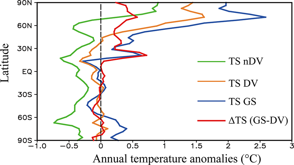
Regional mismatches between models and proxies are a key aspect of the conundrum. Consistent with Bader et al. (Reference Bader, Jungclaus, Krivova, Lorenz, Maycock, Raddatz, Schmidt, Toohey, Wu and Claussen2020), our simulations reveal distinct spatial patterns of temperature evolution. When only Earth orbital forcing is considered (nDV experiment), Mid-Holocene warming is simulated at high latitudes of the Northern Hemisphere, whereas cooling prevails in other regions (Fig. 2, green line). Activating dynamic vegetation (DV experiment) significantly altered this pattern, enhancing warming globally, with the most pronounced effects over the mid- to high latitudes of the Northern Hemisphere (Fig. 2, orange line). The inclusion of Green Sahara forcing in the GS experiment further amplifies warming, particularly across the Northern Hemisphere (Fig. 2, blue line), underscoring the critical role of vegetation feedbacks in shaping regional climate evolution.
Latitudinal profiles of annual temperature anomalies (°C) during the Mid-Holocene (MH) relative to the preindustrial (PI) period from the dynamic vegetation disabled (nDV; green), dynamic vegetation (DV; orange), and Green Sahara (GS; blue) experiments, together with the GS contribution (∆TS) during the MH.

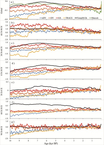
A comparison of simulated and reconstructed Holocene temperature sequences across six 30° latitudinal bands (Fig. 3) reveals that the GS experiment generally aligns most closely with TempM12k, particularly in the Northern Hemisphere. In the high latitudes (60°–90°N), the nDV and TraCE experiments simulate high Mid-Holocene temperatures followed by cooling, whereas the GS experiment yields even higher Mid-Holocene warming (∼2°C above PI levels), exceeding the TempM12k reconstruction by approximately 1°C. The DV experiment shows close agreement with TempM12k in this region.
Reconstructed and simulated annual temperature anomalies (℃) during the Holocene for six 30° latitudinal bands.

Figure 3 Long description
Seven multi-line graphs display reconstructed and simulated annual temperature anomalies in degrees Celsius during the Holocene. The horizontal axis in all panels represents Age in kiloyears Before Present, ranging from 10 to 0. The vertical axis represents temperature anomaly in degrees Celsius, with ranges varying by panel. A shared legend identifies six datasets: nDV, DV, GS, TRACE, TempM12k and Marcott. Panel a, labeled Global, has a vertical axis ranging from negative 0.8 to positive 0.6 degrees Celsius. All six lines cluster closely together, with most datasets showing values near 0 at 0 kiloyears Before Present and slightly negative values around negative 0.2 to negative 0.4 near 10 kiloyears Before Present. TempM12k and Marcott track near 0 throughout, while nDV, DV, GS and TRACE show modest negative departures in the early Holocene. Panel b, labeled 60 degrees to 90 degrees North, has a vertical axis ranging from negative 3.0 to positive 2.0 degrees Celsius. This panel shows the largest spread among datasets. nDV and TRACE reach peaks near positive 1.5 to positive 2.0 degrees Celsius around 9 to 8 kiloyears Before Present, then decline toward 0 or slightly negative by 0 kiloyears Before Present. GS shows an even higher early peak near positive 2.0 degrees Celsius. DV tracks closer to TempM12k, remaining near 0 to positive 1.0 across the record. Marcott stays near 0 throughout. Panel c, labeled 30 degrees to 60 degrees North, has a vertical axis from negative 1.0 to positive 0.6 degrees Celsius. TRACE and GS show positive anomalies near positive 0.5 in the early Holocene, declining toward 0 by present. nDV shows a similar but slightly lower trajectory. DV, TempM12k and Marcott remain near 0 with small fluctuations. Panel d, labeled 0 degrees to 30 degrees North, has a vertical axis from negative 1.0 to positive 0.6 degrees Celsius. Most lines remain close together near 0 to slightly negative. TRACE shows the most negative departure near negative 0.5 to negative 0.8 around 8 to 6 kiloyears Before Present, recovering slightly toward 0 by present. GS and nDV show moderate negative values. DV, TempM12k and Marcott stay closer to 0. Panel e, labeled 30 degrees South to 0 degrees South, has a vertical axis from negative 1.0 to positive 0.5 degrees Celsius. TempM12k shows a prominent positive anomaly near positive 0.5 in the early Holocene, declining steadily to near 0 by present. TRACE, GS and nDV show slightly negative to near-zero values. DV and Marcott remain near 0 throughout. Panel f, labeled 60 degrees South to 30 degrees South, has a vertical axis from negative 1.0 to positive 0.5 degrees Celsius. Most datasets remain near 0 to slightly negative. TRACE shows the most negative values, near negative 0.5 to negative 0.8 in the mid-Holocene. TempM12k and Marcott stay near 0 with minor variation. Panel g, labeled 90 degrees South to 60 degrees South, has a vertical axis from negative 1.0 to positive 0.5 degrees Celsius. Lines show high variability with frequent fluctuations. TRACE and nDV show the largest negative departures near negative 0.5 to negative 1.0 in the early Holocene. GS and DV remain near 0 to slightly negative. TempM12k and Marcott track near 0 throughout.
In the midlatitudes (30°–60°N), the GS experiment corresponds well with the reconstruction, capturing relatively high Early to Mid-Holocene temperatures and a distinct Late Holocene cooling. The DV experiment simulates weak early warming followed by cooling, whereas the nDV experiment shows little trend, and TraCE indicates overall warming throughout the Holocene. In the low latitudes (0°–30°N), only the GS experiment reproduces relatively high Early to Mid-Holocene temperatures and a weak cooling trend, in contrast to the gradual warming simulated in the other experiments. The abrupt temperature decline around 6 ka BP in the GS experiment is associated with the specified termination of the Green Sahara anomaly, consistent with geological evidence (deMenocal et al., Reference deMenocal, Ortiz, Guilderson, Adkins, Sarnthein, Baker and Yarusinsky2000).
In the Southern Hemisphere, model–data discrepancies are more pronounced, especially in the midlatitudes (60°–30°S), likely due to the extensive ocean coverage. However, in both the low latitudes (30°–0°S) and high latitudes (90°–60°S), the inclusion of dynamic vegetation (DV and GS experiments) improves the agreement with TempM12k, with the GS experiment performing most robustly.
Seasonal temperature trends
Seasonal biases in proxies represent another dimension of the conundrum, as certain proxies (e.g., pollen) predominantly record growing season temperatures rather than annual averages. While orbital changes drove a summer cooling and winter warming trend since the Early Holocene, recent evidence from seasonally sensitive proxies (e.g., terrestrial mollusks, dust records) indicates cooling trends in both summer and winter, suggesting seasonal bias alone cannot fully account for the model–data discrepancy (Zhang et al., Reference Zhang, Wu, Cheng, Geng, Li, Sun, Yu, Lu and Guo2022; Jiang et al., Reference Jiang, Zhou, Kok, Lin, Liu, Zhan and Shen2024).
The GS experiment indicates that the Green Sahara contributed to anomalously warm conditions during the Mid-Holocene (Fig. 2). Seasonally, the magnitude of warming in winter exceeded that in summer (Supplementary Fig. S1b). Comparisons of winter (Fig. Supplementary S2) and summer (Fig. Supplementary S3) temperature series show that dynamic vegetation and the Green Sahara increased surface temperatures in both seasons during the Early to Mid-Holocene. The GS experiment produced the highest Early to Mid-Holocene temperatures across the Northern Hemisphere in both seasons compared with other experiments.
In winter, Early to Mid-Holocene warming was most pronounced at high latitudes and weakest in the tropics. The simulated northern high-latitude warming is consistent with the ice-albedo feedback under increased boreal winter insolation. Notably, the relative warmth in the subtropical northern Africa during this period may have been sustained not only by local insolation but also by enhanced Mediterranean winter rainfall, which is hypothesized to be critical for initiating and maintaining Early Holocene greening of the Sahara (Cheddadi et al., Reference Cheddadi, Carré, Nourelbait, François, Rhoujjati, Manay, Ochoa and Schefuß2021; Gaetani et al., Reference Gaetani, Messori, Pausata, Tiwari, Castro and Zhang2024). Our GS experiment, by specifying realistic soil conditions conducive to vegetation, implicitly captures the hydrological preconditioning that such winter rainfall would provide, allowing us to isolate the subsequent warming impact of the vegetated land surface. Following the Mid-Holocene, the Northern Hemisphere experienced cooling, whereas the Southern Hemisphere underwent gradual warming. In summer, enhanced insolation resulted in relatively higher Early to Mid-Holocene temperatures across most regions, except in the mid- to high latitudes of the Southern Hemisphere, where a cooling trend prevailed.
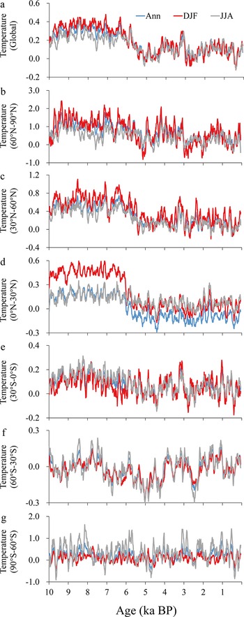
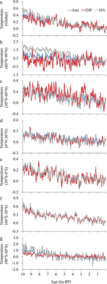
The DV and GS experiments demonstrate that vegetation feedbacks induce surface warming in both winter and summer, thereby modulating the pronounced winter warming trend simulated in TraCE and nDV. The underestimation of land surface feedbacks in previous simulations likely contributes to the seasonally resolved model–data discrepancy. As shown in Figure 4, the difference between GS and DV quantifies the “Green Sahara” contribution, revealing a positive warming effect in both seasons and annually, which is stronger in the Northern Hemisphere and more pronounced in winter than summer. The difference between DV and nDV in Figure 5 further confirms the Early to Mid-Holocene warming effect of dynamic vegetation. This aligns with work done by Liu et al. (Reference Liu, Cheng, Zheng, Zhang, Liu, Wu, Zhu and Xie2025), who emphasized that resolving seasonal temperature biases is critical for reconciling the Holocene temperature conundrum, as seasonal discrepancies in reconstructions are more pronounced over land areas (Mann et al., Reference Mann, Schmidt, Miller and Legrande2009; Osman et al., Reference Osman, Tierney, Zhu, Tardif, Hakim, King and Poulsen2021). The improved performance of the GS and DV experiments in simulating both annual and seasonal temperatures underscores that a realistic representation of vegetation dynamics is critical for resolving the Holocene temperature conundrum.
Temperature anomalies (°C) attributable to the Green Sahara for annual (Ann; blue), winter (DJF; red), and summer (JJA; gray) conditions: (a) global; (b–g) six 30° latitudinal bands.

Figure 4 Long description
Seven multi-line graphs labeled a to g, each representing temperature anomalies in degrees Celsius over time, measured in thousands of years before present (ka BP). The horizontal axis for each graph is labeled Age (ka BP) and ranges from 10 to 0. The vertical axis is labeled Temperature Anomalies (degrees Celsius) and ranges from negative 0.6 to positive 0.6 degrees Celsius. Each graph includes three lines: annual (Ann) in blue, winter (DJF) in red and summer (JJA) in gray. Overall, winter conditions show higher variability and more pronounced peaks compared to summer and annual conditions. Notable peaks in winter occur around 8 ka BP and 3 ka BP, while summer conditions remain relatively stable. Graph a shows winter anomalies peaking at approximately 0.5 degrees Celsius around 8 ka BP. Graph b displays a similar winter peak at 0.4 degrees Celsius around 3 ka BP. Graph c indicates a gradual decline in summer anomalies toward 0 ka BP. Graph d reveals a winter peak at 0.5 degrees Celsius around 5 ka BP. Graph e shows consistent winter fluctuations with peaks at 0.4 degrees Celsius around 7 ka BP. Graph f illustrates a steady pattern with minor winter peaks. Graph g shows minimal variation across all conditions. The graphs collectively demonstrate that winter anomalies tend to be higher and more variable, while summer anomalies are more stable across the latitudinal bands. The data suggests a general trend of decreasing anomalies toward 0 ka BP, particularly in summer conditions.
Temperature anomalies (°C) attributable to terrestrial vegetation (DV minus nDV) for annual (Ann; blue), winter (DJF; red), and summer (JJA; gray) conditions: (a) global; (b–g) six 30° latitudinal bands.

Figure 5 Long description
Seven stacked line graphs labeled a to g, each showing temperature anomalies against age in kiloannum before present. The horizontal axis is labeled ′Age ka BP′ with values from 10 to 1. The vertical axis for each graph represents temperature anomalies in degrees Celsius. The legend identifies three series: Ann (annual), DJF (winter) and JJA (summer). Ann is represented by a blue line, DJF by a red line and JJA by a gray line. Graph a: Temperature anomaly ranges from negative 0.2 to 0.8. Graph b: Ranges from negative 1.0 to 1.5. Graph c: Ranges from negative 0.4 to 0.8. Graph d: Ranges from negative 0.3 to 0.6. Graph e: Ranges from negative 0.2 to 0.4. Graph f: Ranges from negative 0.3 to 0.9. Graph g: Ranges from negative 2.0 to 3.0. Across all graphs, the annual series generally shows less variation compared to winter and summer. Winter series (DJF) often exhibits higher peaks and more pronounced fluctuations, while summer series (JJA) tends to be more stable. Notable peaks and troughs are visible in each graph, indicating periods of significant temperature changes. The graphs illustrate how temperature anomalies have varied over the past 10 thousand years, highlighting differences between seasonal conditions.
Possible mechanisms
Inadequate representation of surface conditions
Multiple paleoclimate reconstructions (Shakun et al., Reference Shakun, Clark, He, Marcott, Mix, Liu, Otto-Bliesner, Schmittner and Bard2012; Marcott et al., Reference Marcott, Shakun, Clark and Mix2013; Kaufman et al., Reference Kaufman, McKay, Routson, Erb, Dätwyler, Sommer, Heiri and Davis2020a, Reference Kaufman, McKay, Routson, Erb, Davis, Heiri and Jaccard2020b) consistently indicate that the global annual mean temperature during the Mid-Holocene (MH, ∼6 ka BP) was approximately 0.5°C warmer than during the PI period. Based on a compilation of over 300 records from Kaufman et al. (Reference Kaufman, McKay, Routson, Erb, Davis, Heiri and Jaccard2020b), we mapped the annual, summer, and winter temperature anomalies for the MH relative to PI (Fig. 6a, Supplementary Fig. S4). Although most proxies suggest a warmer MH, considerable discrepancies are evident among different records, and distinct proxies from the same location can yield conflicting results. Nevertheless, the overall evidence supports a warmer MH. Concurrently, North Africa experienced a humid phase, as indicated by high lake levels and expanded water bodies (Tierney et al., Reference Tierney, Lewis, Cook, Legrande and Schmidt2011; deMenocal et al., Reference deMenocal and Tierney2012; see stars in Fig. 6a and Supplementary Fig. S4d).
The reconstructed surface temperature anomalies (°C) and African lake levels during the Mid-Holocene (MH) relative to the preindustrial (PI) period, and the surface temperatures, vegetation coverage, albedo, and net radiation obtained from numerical simulations. (a) Reconstructed annual surface temperature (circles; Kaufman et al., Reference Kaufman, McKay, Routson, Erb, Dätwyler, Sommer, Heiri and Davis2020a; NOAA template format) and African lake levels (stars; Tierney et al., Reference Tierney, Lewis, Cook, Legrande and Schmidt2011; deMenocal et al., Reference deMenocal and Tierney2012). Brown denotes warmer temperatures or higher lake levels, and blue indicates cooler temperatures or lower lake levels. (b) Results from 13 Paleoclimate Modeling Intercomparison Project (PMIP4) models, EC-Earth (Chen et al., Reference Chen, Zhang, Lu, Duan, Cao, Huang and Chen2024), TraCE (Liu et al., Reference Liu, Zhu, Rosenthal, Zhang, Otto-Bliesner, Timmermann, Smith, Lohmann, Zheng and Timm2014), and the dynamic vegetation disabled (nDV), dynamic vegetation (DV), and Green Sahara (GS) experiments. (c–f) Differences in annual temperature (TS; ℃), total vegetation percentage (TotalVeg; %), surface albedo (Albedo; %), and surface net solar radiation (SNR; W/m2). Gray hatching indicates areas where anomalies are statistically significant at the 99% confidence level (two-tailed t-test, all subsequent panels adopt identical statistical settings).

Figure 6 Long description
The image A titled Ann TS NOAA shows a world map with circular and star markers indicating reconstructed annual surface temperature anomalies and African lake levels. The map uses latitude labels 90N, 45N, EQ, 45S, 90S and longitude labels 90W, 0, 90E, 180E. Warm colors indicate positive anomalies, while cool colors indicate negative anomalies. The image B titled Ann TS PMIP4 presents a bar chart comparing temperature anomalies from various PMIP4 models. The x-axis lists models such as ACCESS ESM1 5, AWI ESM 1 1 LR and others, while the y-axis ranges from 0.3 to negative 0.3. Most models show negative anomalies, with GS showing positive anomalies. The image C titled Ann TS GS displays a global map of temperature anomalies with a scale from negative 2 to 2 degrees Celsius. Warm colors indicate positive changes, concentrated in northern regions, while cool colors indicate negative changes. The image D titled Ann TotalVeg GS shows a global map of vegetation percentage anomalies with a scale from negative 20 to 20 percent. Positive changes are concentrated in tropical regions, while negative changes appear in northern areas. The image E titled Ann Albedo GS presents a global map of albedo anomalies with a scale from negative 5 to 5 percent. Positive changes are seen in polar regions, while negative changes occur in equatorial areas. The image F titled Ann SNR GS shows a global map of net solar radiation anomalies with a scale from negative 20 to 20 W m superscript negative 2. Positive changes are concentrated in northern regions, while negative changes are seen in southern areas. These maps illustrate differences between observations, model ensembles and GS products, highlighting temperature changes alongside vegetation, albedo and radiation shifts.
Analyses of the Paleoclimate Modeling Intercomparison Project (PMIP) simulations, which use specified MH orbital parameters and greenhouse gas concentrations, reveal that nearly all models simulate cooler global annual temperatures compared with PI. Only a few models show slight warming, even at a regional scale (Jiang et al., Reference Jiang, Lang, Tian and Wang2012; Tian et al., Reference Tian and Jiang2015). Within the PMIP4 ensemble (see model details in Supplementary Table S1), MH temperatures are generally lower than PI values (Fig. 6b, Supplementary Fig. S5), with global annual anomalies ranging from −0.52°C (FGOALS-f3-L) to −0.13°C (CESM2). The 13-model ensemble mean indicates the MH was approximately 0.33°C cooler than the PI. Spatially, most models simulate warming at high latitudes in both hemispheres but significant cooling in mid- and low latitudes, highlighting a systematic model–data discrepancy outside the polar zones.
Recent studies have demonstrated that afforestation reduces surface albedo, thereby increasing solar energy absorption and raising surface temperatures (Kristensen et al., Reference Kristensen, Barbero-Palacios, Barrio, Jacobsen, Kerby, López-Blanco and Malhi2024; Li et al., Reference Li, Wang and Chen2024). During the MH, North Africa was characterized by grasslands, shrubs, forests, and lakes, a landscape known as the Green Sahara, supported by precipitation levels nearly 10 times higher than those of PI period (Kutzbach and Liu, Reference Kutzbach and Liu1997; Tierney et al., Reference Tierney, Pausata and deMenocal2017). These changes would have significantly altered land conditions and associated climate feedbacks. However, nearly all PMIP simulations specify PI land surface conditions, thereby failing to account for the Green Sahara (Kuper and Kröpelin, Reference Kuper and Kröpelin2006; Drake et al., Reference Drake, Blench, Armitage, Bristow and White2011). This omission likely contributes to the simulated MH cooling bias in most models.
Terrestrial vegetation feedback
Our idealized simulations demonstrate that incorporating vegetation feedbacks reconciles temperature differences between models and proxy reconstructions (Figs. 6b and 7). The global annual Mid-Holocene to PI (MH-PI) temperature anomalies are −0.15°C (nDV), 0.07°C (DV), and 0.28°C (GS) compared with −0.32°C simulated in the TraCE full-forcing experiment (Liu et al., Reference Liu, Zhu, Rosenthal, Zhang, Otto-Bliesner, Timmermann, Smith, Lohmann, Zheng and Timm2014). Spatially, the inclusion of dynamic vegetation results in widespread warming across mid- to high latitudes of the Northern Hemisphere during the MH (Fig. 7). The GS experiment, which incorporates Green Sahara forcing, yields pronounced warming over North Africa and most other regions (Fig. 6c). These findings align with those of Chen et al. (Reference Chen, Zhang, Lu, Duan, Cao, Huang and Chen2024), who reported MH-PI anomalies of −0.06°C (orbital forcing), 0.15°C (vegetation forcing), and 0.10°C (combined forcing).
Temperature anomalies (℃) and the contribution of surface condition changes during the Mid-Holocene (MH) relative preindustrial (PI) period. (a and c) Temperature anomalies from the EC-Earth (Chen et al., Reference Chen, Zhang, Lu, Duan, Cao, Huang and Chen2024) and dynamic vegetation (DV) experiments; (b and d) Contributions from terrestrial vegetation and the Green Sahara, respectively.

Figure 7 Long description
Four global thematic heat maps illustrate near-surface temperature anomalies in degrees Celsius during the Mid-Holocene compared to the preindustrial period. North is oriented at the top. The maps are divided into panels A-D. Panel A, labeled ′Ann TS EC-Earth_All′, shows anomalies ranging from -2 to 2 degrees Celsius, with cooler regions in blue and warmer regions in orange and red. Panel B, ′Delta Veg′, highlights vegetation effects, showing warming in mid to high latitudes. Panel C, ′Ann TS DV′, presents dynamic vegetation impacts, similar to Panel A. Panel D, ′Delta Green Sahara′, emphasizes warming over North Africa. The legend uses a continuous scale from -2 to +2 degrees Celsius, centered at 0 degrees Celsius, representing anomalies from a baseline. Latitude and longitude lines are marked, aiding orientation. Cooling is prominent in oceanic regions, while warming hotspots appear in continental areas, especially North Africa in Panel D.
Both our DV experiment and the precipitation-enhanced vegetation experiment conducted by Chen et al. (Reference Chen, Zhang, Lu, Duan, Cao, Huang and Chen2024) simulate warmer MH conditions relative to PI, yet neither yields significant greening in the Sahara. The underestimation of vegetation cover, likely attributable to unrealistic soil properties in the model, is a primary cause of the cool bias in simulated MH temperatures. By incorporating vegetation dynamics, GS successfully simulates Early to Mid-Holocene warming and subsequent cooling, consistent with proxy reconstructions. In GS, the adjustment of Saharan soil properties ideally reproduces Green Sahara conditions. During the PI period, the DV experiment indicates that the Saharan region (20°W–30°E, 10°N–20°N) was 72.36% barren, with 25.79% C4 grass and 1.85% needleleaf evergreen trees (TempNET); temperate broadleaf deciduous shrubs (TempBDS) were absent. By the MH, DV simulations show barren cover decreased to 67.72%, C4 grass coverage reduced to 12.47%, and two competitive vegetation types expanded: TempBDS emerged with 11.19% coverage, and TempNET increased to 8.62%. The GS experiment further reduces barren area to 59.17% and C4 grass to 11.07% during the MH, while TempBDS expands to 22.82%, consistent with reconstructions (Jolly et al., Reference Jolly, Prentice, Bonnefille, Ballouche, Bengo, Brenac and Buchet1998; Hoelzmann et al., Reference Hoelzmann, Jolly, Harrison, Laarif, Bonnefille and Pachur1998; Fig. 8). TempNET in GS slightly decreases to 6.94% but remains substantially higher than in the PI period.
The terrestrial vegetation distribution of North Africa during the preindustrial (PI) period and Mid-Holocene (MH) from the dynamic vegetation (DV), and Green Sahara (GS) experiments. The Community Earth System Model (CESM1.2) DV module outputs 13 vegetation types and barren land: temperate needleleaf evergreen tree (TempNET), boreal needleleaf evergreen tree (BorealNET), tropical broadleaf evergreen tree (TropBET), temperate broadleaf evergreen tree (TempBET), tropical broadleaf deciduous treen (TropBDT), temperate broadleaf deciduous tree (TempBDT), boreal broadleaf deciduous tree (BorealBDT), temperate broadleaf deciduous shrub (TempBDS), boreal broadleaf deciduous shrub (BorealBDS), C3 arctic grass (ArcticC3), C3 grass (C3), C4 grass (C4), and barren (Barren). In North Africa, in the PI and MH periods, except for several major vegetation types shown in this figure, the distribution of other vegetation was close to 0 or equal to 0, as represented by others.

Figure 8 Long description
A pie chart labeled, PI. Slice labels read, Barren 72.36 percent, C4 25.79 percent, TempNET 1.85 percent, Others 0.00 percent. The image B showing a pie chart labeled, DV underscore MH. Slice labels read, Barren 67.72 percent, C4 12.47 percent, TempBDS 11.19 percent, TempNET 8.62 percent, Others 0.00 percent. The image C showing a pie chart labeled, GS underscore MH. Slice labels read, Barren 59.17 percent, TempBDS 22.82 percent, C4 11.07 percent, TempNET 6.94 percent, Others 0.00 percent. A legend lists, Barren, BorealNET, TempBET, TempBDT, TempBDS, ArcticC3, C4, TempNET, TropBET, TropBDT, BorealBDT, BorealBDS, C3, Others.
Enhanced vegetation during the MH, particularly associated with the Green Sahara, exerted a significant influence on temperatures. Increased summer insolation amplified vegetation cover across the Northern Hemisphere (Fig. 9a). The GS experiment simulated further vegetation expansion, especially pronounced in the Saharan region (Figs. 6d and 9b), leading to increased terrestrial vegetation and leaf area index (Fig. 9c and d). Relative to DV, GS demonstrates that the Green Sahara not only enhanced local vegetation but also promoted growth across the Northern Hemisphere, thereby reducing surface albedo (Figs. 6e and 9f) and increasing surface net solar radiation (SNR; Figs. 6f and 9h). The GS experiment also captured a substantial increase in annual precipitation over the Sahara, rising from 40.45 mm/yr during the PI to 362.05 mm/yr during the MH, an approximately ninefold increase consistent with proxy evidence (Tierney et al., Reference Tierney, Pausata and deMenocal2017), compared with only 130.51 mm/yr simulated for the MH under the DV experiment (Fig. 10). These results underscore that the omission of the Green Sahara and its associated climate feedback in previous modeling studies likely explains their failure to reproduce MH warming and the subsequent cooling trend evident in proxy records.
The differences in annual total vegetation percentage (Ann TotalVeg; %), total leaf area index (Ann TLAI), surface albedo (Ann Albedo; %), surface net solar radiation (Ann SNR; W/m2). Left panels show the difference between Mid-Holocene (MH) relative preindustrial (PI) periods from dynamic vegetation (DV) experiments; right panels show the Green Sahara (GS) contribution during the MH.

Figure 9 Long description
Thematic world map grid with eight sub-images arranged in four rows and two columns. Each sub-image has latitude labels at 90N, 45N, Eq, 45S, 90S and longitude labels at 180W, 90W, 0, 90E, 180E. North is at the top. The left column maps are labeled with dynamic vegetation and the right column maps are labeled as Green Sahara minus dynamic vegetation. A) Ann TotalVeg DV. Legend labeled percent with tick labels 0, 5, 10, 15, 20. Land areas show mixed positive and negative patches, with many positive patches across northern Africa, parts of the Middle East, parts of South Asia, parts of East Asia and parts of North America. Smaller mixed patches appear in South America and Australia. B) Ann TotalVeg (GS minus DV). Legend labeled percent with tick labels 0, 5, 10, 15, 20. A broad positive area spans northern Africa, with additional scattered positive patches across parts of the Middle East and parts of Asia. Many other land areas show weaker or patchier changes. C) Ann TLAI DV. Legend labeled 0.0, 0.1, 0.2, 0.3, 0.4, 0.5. Land areas show scattered patches of higher and lower values across northern Africa, parts of the Middle East, parts of South Asia, parts of East Asia and parts of North America, with smaller patches in South America and Australia. D) delta TLAI (GS minus DV). Legend labeled 0.0, 0.1, 0.2, 0.3, 0.4, 0.5. A concentrated positive area appears across northern Africa, with additional smaller positive patches in parts of the Middle East and parts of Asia. E) Ann Albedo DV. Legend labeled percent with tick labels minus 4, minus 3, minus 2, minus 1, 0, 1, 2, 3, 4. Large areas of the high northern latitudes show negative values, while many lower latitude land areas show mixed small positive and negative patches. F) Ann Albedo (GS minus DV). Legend labeled percent with tick labels minus 4, minus 3, minus 2, minus 1, 0, 1, 2, 3, 4. Northern Africa shows a prominent negative area, with additional scattered negative patches in parts of the Middle East and parts of Asia. Other regions show smaller mixed patches. G) Ann SNR DV. Legend labeled W m superscript minus 2 with tick labels minus 30, minus 20, minus 10, 0, 10, 20, 30. Broad areas show mixed positive and negative patches across land and ocean, with notable patchiness across the Northern Hemisphere. H) Ann SNR (GS minus DV). Legend labeled W m superscript minus 2 with tick labels minus 30, minus 20, minus 10, 0, 10, 20, 30. Northern Africa shows a prominent positive area, with additional scattered positive patches in parts of the Middle East and parts of Asia, while other regions show weaker mixed patches.
The anomalies and differences in annual precipitation (mm/day); winter (DJF) and summer (JJA) 850 hPa wind fields (m/s); and the contribution of the Green Sahara (GS). Left columns show the difference between Mid-Holocene (MH) relative preindustrial (PI) periods from dynamic vegetation (DV) experiments; right columns show the GS contribution during the MH. For clarity, the 850 hPa winds are displayed only where anomalies are statistically significant at the 99% confidence level (two-tailed t-test).

Figure 10 Long description
Insufficient visual information to describe this element accurately.
The presence of the Green Sahara also perturbed large-scale atmospheric circulation patterns. Results from the DV experiment indicate that both the North African summer monsoon (NASM) and the East Asian summer monsoon (EASM) were significantly intensified (Fig. 10e) during the MH relative to the PI. In the GS experiment, the establishment of the Green Sahara further reinforced the NASM (Fig. 10f), while the EASM also exhibited an enhancement, albeit one that did not pass the 95% significance test. This enhancement was primarily driven by reduced surface albedo associated with the expansion of vegetation over the Sahara (Figs. 6e and 9e and f), which in turn increased SNR (Figs. 6f and 9g and h) and induced substantial surface warming over the Saharan region (Fig. 7). The pronounced surface warming over the Sahara acted as a local heat source, driving atmospheric circulation adjustments that facilitated global energy redistribution and led to elevated temperatures across much of the Northern Hemisphere. While the associated teleconnections to the EASM are not evident in the 850 hPa wind field analysis at the 99% confidence level (Fig. 10f), the Saharan heat source may still modulate EASM activity via upper-tropospheric wave trains or tropical interbasin interactions. Consequently, the Green Sahara played a critical role in modulating MH climate, an effect that remains inadequately represented in current generation PMIP-style simulations.
Discussion
The accurate simulation of Holocene temperature trends in the GS experiment, an idealized sensitivity study designed to isolate the role of a vegetated Sahara, provides critical insights into the “Holocene temperature conundrum” and strengthens the reliability of proxy-based reconstructions that have been subject to debate. Our findings suggest that the Late Holocene cooling trend observed in proxies, which has long eluded model reproduction, may stem from the inability of earlier simulations to reproduce Early to Mid-Holocene warming, particularly during the Green Sahara epoch. This Late Holocene cooling is closely linked to the reestablishment of desert conditions and the rapid decline in vegetation cover. The de-desertification process during the Early to Mid-Holocene, when considered through the lens of soil–vegetation–atmosphere coupling (rather than vegetation alone), may therefore hold a key complementary perspective for resolving the long-standing model–data discrepancy. Consistent with Hopcroft and Valdes (Reference Hopcroft and Valdes2022), our transient framework captures the Sahara’s abrupt desertification as a threshold-dependent response: when vegetation cover drops below a critical level (∼30% in our simulation), weakened moisture recycling and disrupted albedo feedbacks trigger rapid drying. This finding is echoed by the transient Earth system model simulations of the German PALMOD group (Dallmeyer et al., Reference Dallmeyer, Claussen, Lorenz and Shanahan2020), which documented the termination of the African humid period and its climatic impacts over the last 8000 years, thus offering independent support for the link between Saharan desertification and Late Holocene cooling identified in our GS experiment.
Notably, this model–data discrepancy is composite in nature, arising from multiple factors. While our study highlights the pivotal role of insufficient vegetation–land surface interaction, recent studies highlight that many Holocene temperature proxies may carry a persistent seasonal bias, potentially overrepresenting warm-season conditions (Bova et al., Reference Bova, Rosenthal, Liu, Godad and Yan2021; Marshall et al., Reference Marshall, Morrill, Dee, Jiang, Kim and Russell2025). Marshall et al. (Reference Marshall, Morrill, Dee, Jiang, Kim and Russell2025) further note that proxy system biases, such as seasonal preservation biases and geochemical calibration errors, could explain up to 80% of Mid-Holocene temperature mismatches in tropical East Africa. Their work also indicates that Green Sahara–induced dust reduction enhanced surface shortwave radiation, contributing an additional ∼0.3℃ warming in tropical lakes, a secondary pathway complementing our vegetation–albedo–precipitation feedback. Such inherent limitation in proxy data could partly explain the apparent model–data discrepancy and serve as an important caveat to our model-based conclusions. Determining the relative contributions of proxy seasonal bias versus missing feedbacks in models therefore remains a key challenge for future research.
Mechanisms identified in the GS experiment, such as vegetation–albedo feedbacks and Arctic amplification, further explain why vegetation-induced warming is more pronounced in winter than in summer. It should be emphasized that the GS represents an idealized scenario in which soil properties were specified to their non-desert counterparts, allowing us to evaluate the maximum potential climate impact of a Green Sahara. This vegetation expansion represents only one component of the broader Green Sahara phenomenon, which also includes shifts in soil properties and ecosystem structure. If our interpretation holds, this idealized experimental framework offers a valuable reference for implementing realistic Green Sahara boundary conditions in future Holocene climate simulations.
Our findings align with previous research that identified vegetation–climate feedbacks as a key factor in Holocene climate evolution (e.g., Bonan, Reference Bonan2008; Pausata et al., Reference Pausata, Zhang, Muschitiello, Lu, Chafik, Niedermeyer, Stager, Cobb and Liu2017) but extend these insights by explicitly quantifying the role of the Green Sahara’s land surface conditions. Chen et al. (Reference Chen, Zhang, Lu, Duan, Cao, Huang and Chen2024) simulated Mid-Holocene warming via vegetation forcing but did not capture significant Saharan greening due to unrealistic soil parameterizations, leading to a more modest global temperature anomaly (+0.15°C) compared with our GS experiment (+0.28°C). By contrast, our DV experiment uses the fully coupled CESM1.2 with a standard dynamic vegetation module, while our GS experiment builds on DV by specifying realistic Saharan soil property adjustments (e.g., increased soil water-holding capacity, modified texture) to emulate the non-desert land surface conditions of the Green Sahara—an experimental design innovation that isolates the maximum climate impact of Saharan greening, a process not explicitly represented in EC-Earth (Chen et al., Reference Chen, Zhang, Lu, Duan, Cao, Huang and Chen2024). Unlike Swann et al. (Reference Swann, Fung, Liu and Chiang2014), who specified Green Sahara vegetation cover, our approach modifies soil properties to allow spontaneous vegetation expansion, preserving critical vegetation–climate coupling and providing a more realistic representation of the feedback mechanisms driving Holocene temperature trends.
In this study, external forcings were limited to orbital variations and greenhouse gas changes. For the land component, a dynamic vegetation module was activated, and Saharan soil properties were adjusted to emulate Green Sahara conditions in this idealized experiment. Nevertheless, Holocene climate evolution arises from the interplay of multiple forcings and internal feedbacks, many of which are indirectly recorded in proxies but only partially represented in models. This incomplete representation remains a major source of model–data divergence.
For example, Early to Mid-Holocene ice-sheet retreat (Liu et al., Reference Liu, Zhu, Rosenthal, Zhang, Otto-Bliesner, Timmermann, Smith, Lohmann, Zheng and Timm2014) and associated sea-ice changes likely exerted considerable influence on Holocene temperature evolution (Park et al., Reference Park, Kim, Stewart, Son and Seo2019; Bader et al., Reference Bader, Jungclaus, Krivova, Lorenz, Maycock, Raddatz, Schmidt, Toohey, Wu and Claussen2020; Zhou et al., Reference Zhou, Li, Shi, Sha, Lei and An2023). Similarly, dust cycle feedbacks, strongly modulated by vegetation cover, play important direct and indirect roles in climate (Hoelzmann et al., Reference Hoelzmann, Jolly, Harrison, Laarif, Bonnefille and Pachur1998; Liu et al., Reference Liu, Zhang, Liu, Xia, Huang, Peng and Zhu2018; Jiang et al., Reference Jiang, Zhou, Kok, Lin, Liu, Zhan and Shen2024). Marshall et al. (Reference Marshall, Morrill, Dee, Pausata and Russell2024) further clarify that Mid-Holocene African temperatures in PMIP simulations are co-regulated by orbital forcing, dust, and monsoons—all linked to the Green Sahara. They also note PMIP4 models are cooler than PMIP3 models due to greenhouse gas (GHG) differences, partly explaining traditional models’ failure to simulate Mid-Holocene warming, which aligns with our finding that Green Sahara feedbacks compensate for this cool bias. Moreover, land surface changes concurrent with the Green Sahara in other regions may also have left a significant imprint (Hou et al., Reference Hou, Long, Tsukamoto, Lu, Chen, Ibarra and Tamura2024).
It is important to address the paleo calendar effect in transient Holocene simulations (Bartlein and Shafer, Reference Bartlein and Shafer2019). This effect can shift the timing of local temperature maxima/minima by hundreds to thousands of years, with seasonal variability. While we did not perform adjustments (due to substantial effort), it may introduce minor temporal offsets in our GS experiment’s results—particularly for seasonally resolved trends. However, because our core focus is on the magnitude and direction of vegetation–climate feedbacks, this effect does not fundamentally alter our conclusion that the Green Sahara resolves the Holocene temperature conundrum. Future work could use PaleoCalAdjust v1.0 (Bartlein and Shafer, Reference Bartlein and Shafer2019) to refine temporal precision.
Although the GS experiment reproduces the broad temporal pattern of Holocene temperatures in close agreement with reconstructions, it should be noted that this is an idealized simulation. Regional discrepancies persist, particularly between hemispheres and across latitude bands, indicating that the Holocene temperature conundrum cannot be fully resolved without further coordinated modeling and proxy-based studies, especially as Liu et al. (Reference Liu, Cheng, Zheng, Zhang, Liu, Wu, Zhu and Xie2025) underscore that seasonal dynamics are a core, underaddressed dimension of the discrepancy and Dallmeyer et al. (Reference Dallmeyer, Claussen, Lorenz and Shanahan2020) highlight the value of transient simulations for capturing the full complexity of African humid period termination. Future work should therefore integrate global land surface changes alongside the Green Sahara, including dust–climate–vegetation feedbacks, to more comprehensively capture the processes that shaped Holocene climate evolution. Building on Marshall et al. (Reference Marshall, Morrill, Dee, Pausata and Russell2024, Reference Marshall, Morrill, Dee, Jiang, Kim and Russell2025), Liu et al. (Reference Liu, Cheng, Zheng, Zhang, Liu, Wu, Zhu and Xie2025), Dallmeyer et al. (Reference Dallmeyer, Claussen, Lorenz and Shanahan2020), and Bartlein and Shafer (Reference Bartlein and Shafer2019), combining dynamic vegetation/proxy system models, dust–vegetation feedbacks, seasonal resolution, and paleo calendar–adjusted transient frameworks will disentangle multifactor contributions and address key dimensions of the conundrum.
Conclusion
In this study, we conducted a set of transient Holocene simulations, including an idealized sensitivity experiment (GS) that incorporated dynamic vegetation and a realistic representation of the Green Sahara during the Early to Mid-Holocene. Our experiments successfully reproduced the long-term temperature evolution documented in proxy records, demonstrating that vegetation–climate feedbacks are essential for simulating Holocene climate evolution.
The dynamic vegetation experiment (DV) simulated a Mid-Holocene global mean temperature 0.07°C warmer than PI levels, consistent with the 0.10°C warming reported in EC-Earth time-slice experiments (Chen et al., Reference Chen, Zhang, Lu, Duan, Cao, Huang and Chen2024). The idealized Green Sahara experiment (GS) further enhanced this warming, yielding a Mid-Holocene anomaly of 0.28°C, which is closer to the 0.37°C warming indicated by Marcott et al. (Reference Marcott, Shakun, Clark and Mix2013). As an idealized scenario, the GS experiment also captured a nearly ninefold increase in annual precipitation over the Sahara, reaching 362.05 mm/yr during the Mid-Holocene, in agreement with geological evidence (Tierney et al., Reference Tierney, Pausata and deMenocal2017).
Spatially, this idealized GS experiment simulated a gradual temperature rise from the Early to Mid-Holocene across most of the Northern Hemisphere, followed by Late Holocene cooling, a pattern consistent with proxy reconstructions. Seasonally, the vegetation expansion in this idealized scenario led to greater winter warming than summer warming, elevating Early to Mid-Holocene winter temperatures and improving the agreement with proxy records. This result aligns with recent seasonally resolved records (Dong et al., Reference Dong, Wu, Li, Zhang, Zhang, Shen and Lu2022; Jiang et al., Reference Jiang, Zhou, Kok, Lin, Liu, Zhan and Shen2024).
In summary, the implementation of this idealized Green Sahara scenario in our transient Holocene simulations improves the agreement between models and paleoclimate reconstructions at multiple scales and provides new insights into the role of vegetation–climate interactions. The greening and subsequent desertification of the Sahara, as characterized in this idealized experiment, are identified as key processes shaping hemispheric and seasonal climate trends throughout the Holocene. This study highlights the value of using idealized experiments to isolate and quantify the effects of specific boundary conditions in paleoclimate modeling.
Supplementary material
The supplementary material for this article can be found at https://doi.org/10.1017/qua.2026.10116.
Acknowledgments
This work was supported by the National Key R&D Program of China (2023YFF0804804), the National Natural Science Foundation of China (42575053), the Science and Technology Innovation Project of Laoshan Laboratory (LSKJ202203300), and CIRP Open Fund of Radiation Protection Laboratories (ZFYFSHJ-2023001).
Data Availability Statement
All measured proxy indices and simulated data presented in this study are provided in Supplementary Datasets 1 and 2. These datasets will be permanently archived and made publicly available upon publication through the East Asian Paleoenvironmental Science Database (https://doi.org/10.12262/IEECAS.EAPSD2025002). Supplementary Dataset 1 contains Mid-Holocene temperature anomalies relative to the PI period, organized following the NOAA template format of Kaufman et al. (Reference Kaufman, McKay, Routson, Erb, Davis, Heiri and Jaccard2020b). The dataset comprises three tables (Annual, Summer, Winter) with the following fields: (1) Dataset Name; (2) Site Name; (3) Country/Ocean; (4) Latitude (°); (5) Longitude (°); (6) Elevation (m); and (7) Cold/Warm classification for the Mid-Holocene. Supplementary Dataset 2 also includes three corresponding tables (Annual, Summer, Winter) containing the global mean temperature series and six 30° latitudinal band series from the nDV, DV, and GS experiments, along with their corresponding calendar ages (ka BP).
Competing Interests
The authors declare no competing interests.



 Open access

