1. Introduction
Thermocapillary convection flows, driven by thermocapillary forces induced by temperature gradients on liquid–liquid or liquid–gas interfaces, are prevalent in various natural and industrial processes and play a critical role at microgravity condition and in micro- and nano-scale environments such as in 3D printing (Wei et al. Reference Wei, Wang, Shin and Rong2018), space welding (Liu et al. Reference Liu, Dong, Wang and Chen2021), laser surface melting (Seidgazov Reference Seidgazov2009), swimming actuators (Hou et al. Reference Hou, Guan, Li, Sun, Long and Song2021) and micro-robotics (Piñan Basualdo et al. Reference Piñan Basualdo, Bolopion, Gauthier and Lambert2021). Accordingly, the study of thermocapillary convection flows is of practical significance and is of fundamental importance in the field of fluid mechanics.
Over the past decades, thermocapillary convection flows generated by a heated vertical wall or a heated sidewall of a cavity have received considerable attention. It is expected that a thermal boundary layer may form adjacent to a suddenly heated vertical wall (Patterson & Imberger Reference Patterson and Imberger1980; Cowley & Davis Reference Cowley and Davis1983). Further, temperature gradient-induced thermocapillary forces may drive a surface flow (Villers & Platten Reference Villers and Platten1992) and generate a pressure gradient in the vertical direction, which also induces a flow along the vertical wall (Sen & Davis Reference Sen and Davis1982). Different dynamical evolutions of transient thermocapillary convection flows with unique characteristics have been identified for heating conditions such as isothermal heating (Chen & Xu Reference Chen and Xu2021a ), iso-flux heating (Chen & Xu Reference Chen and Xu2021b ) and ramp heating (Chen & Xu Reference Chen and Xu2023) of the vertical wall. The thicknesses and velocity scales of the corresponding boundary layer have been obtained.
Apart from the flat vertical wall, thermocapillary convection flows induced by a heated curved wall are common in nature and industrial applications such as the thermal-probe microscope (Aigouy et al. Reference Aigouy, Lalouat, Mortier, Löw and Bergaud2011), fabrication of crystals (Peng et al. Reference Peng, Li, Shi and Imaishi2007) or laser beams (Wei et al. Reference Wei, Wang, Shin and Rong2018; Xu et al. Reference Xu, Zou, Liu, Wang and Kang2022), which have also received considerable attention due to diverse flow structures. The curvature of the heated curved wall introduces fundamental geometrical modifications to the dynamical evolution and thermal process of transient thermocapillary convection flows substantially different from those induced by the flat vertical wall. For instance, in an annular liquid pool, the curvature may change the stability of thermocapillary convection flows in which various flow modes have been observed for different curvature values (Imaishi, Ermakov & Shi Reference Imaishi, Ermakov and Shi2020; Khan & Bera Reference Khan and Bera2020).
Scaling analysis is an effective method to understand thermocapillary convection flows in the symmetric configuration, such as a pool melted by a laser (Xu et al. Reference Xu, Zou, Liu, Wang and Kang2022). It has been demonstrated that thermocapillary convection flows are composed of four regions in a cylindrical cavity: a free surface boundary layer, a core region, a corner region and a sidewall boundary layer for which the relationships between the flow and the surface tension Reynolds number (
 $ \textit{Re}_{\sigma} $
) and Marangoni number (Ma) are proposed. Kamotani, Chang & Ostrach (Reference Kamotani, Chang and Ostrach1996) also established the critical relationship for steady thermocapillary convection flows in a cylindrical pool. By comparing isothermal and isoflux heating ways, the velocity has been proposed from viscous-dominated to inertia-dominated regimes, and the Nusselt number for the convection-dominated heat transfer (Nu ∼ Ma
 $ ^{1/3} $
,
 $Nu = hL/k$
,
 $Ma = {\alpha_{T}}{\Delta}TL/({\mu}{\kappa})$
, where
 $h$
denotes the convective heat transfer coefficient,
 $L$
refers to the characteristic length,
 $k$
represents the thermal conductivity,
 ${\alpha_{T}}$
denotes the temperature coefficient of surface tension,
 ${\Delta}T$
refers to the characteristic temperature difference,
 $\mu$
and
 $\kappa$
represent the dynamic viscosity and thermal diffusivity of the working fluid) for high Marangoni numbers. Kamotani & Ostrach (Reference Kamotani and Ostrach1998) has further presented the scaling laws of the non-dimensional characteristic hot corner velocity (
 $ U_{0}^{*} $
∼ Ma
 $ ^{-1/7} $
,
 $U_{0}^{*} = {\mu}U_0/({\alpha_{T}}{\Delta}T)$
, where
 $U_0$
denotes the characteristic velocity in the hot corner region) and Nusselt number (Nu ∼ Ma
 $ ^{2/7} $
) during the oscillations for a high Prandtl number (Pr). Additionally, experimental results also show that the surface distortion modifies the thermocapillary force (Kamotani, Ostrach & Masud Reference Kamotani, Ostrach and Masud1999).
The above studies indicate that there are significant differences between thermocapillary convection flows in the cylindrical and rectangular pools. Unfortunately, the impact of the curvature on thermocapillary convection flows is still unclear. However, it has been demonstrated that the curvature of a heated vertical cylinder substantively changes buoyant convection flows, resulting in a significant increase of the Nusselt number in previous studies (Cebeci, Wogulis & Partin Reference Cebeci, Wogulis and Partin1968; Khouaja, Chen & Armaly Reference Khouaja, Chen and Armaly1991). In buoyant convection flows, the correlation between the Nusselt number and curvature has been explored, emphasising the importance of the curvature in heat transfer (Kang, Chung & Kim Reference Kang, Chung and Kim2014; Goodrich & Marcum Reference Goodrich and Marcum2019; Zhao, Lei & Patterson Reference Zhao, Lei and Patterson2021). In the case in which the cylinder is thick and its diameter is much larger than the thickness of the thermal boundary layer (D > > δ
T
), heat transfer is similar to that adjacent to a vertical flat plate, scaled by the classical scaling law of Nu ∼ Ra
 $ ^{1/4} $
, where Ra denotes the Rayleigh number (Touloukian, Hawkins & Jakob Reference Touloukian, Hawkins and Jakob1948; Bottemanne Reference Bottemanne1972; Kang et al. Reference Kang, Chung and Kim2014). In the case in which the cylinder is thin and its diameter is equal to or smaller than the thickness of the thermal boundary layer (D ≈ δ
T
or D < < δ
T
), the curvature effect is pivotal and there exists a positive Nu–curvature correlation (Sparrow & Gregg Reference Sparrow and Gregg1956), which is validated by experimental results for non-dimensional height
 $ H/D $
< 60, where H is the height of cylinder (Popiel, Wojtkowiak & Bober Reference Popiel, Wojtkowiak and Bober2007). Further analysis of the curvature effect on heat transfer (Zhao et al. Reference Zhao, Lei and Patterson2021) and transient buoyant convection flows (Liu & Liu Reference Liu and Liu2022) around the vertical cylinder has been performed. The cross-sectional expansion of the annular thermal boundary layer around a heated wire due to the curvature effect may be a determining factor in heat transfer (Zhang Reference Zhang2025).
Based on the above literature review, a quantitative analysis of the curvature effect on thermocapillary convection flows is to be expected. In particular, the curvature effect could play a critical part in understanding of transient thermocapillary convection flows around a suddenly heated vertical wire, which could further bring about a novel perspective on the surface flow in the cylindrical coordinate system. Accordingly, this study employs scaling analysis and axisymmetric numerical simulation to investigate transient flows around a suddenly heated vertical wire. We find four possible dynamical evolutions of transient thermocapillary convection flows around the suddenly heated vertical wire, which are rarely investigated in previous studies in a rectangular pool (Chen & Xu Reference Chen and Xu2021a ; Chen & Xu Reference Chen and Xu2021b ; Meng, Chen & Xu Reference Meng, Chen and Xu2024a ). New scaling laws have been proposed under different regimes in different dynamic evolutions, which are also validated by numerical results. The insights gained from this study may be applied for the transient behaviour of fluid flows in a thermal-probe microscope and the fabrication of crystals.
The structure of the paper is outlined as follows. Section 2 provides the description of the physical problem. Section 3 performs a scaling analysis for transient flows near a suddenly heated wire. The methodology of numerical simulation is described in § 4. Section 5 presents numerical results and validations against scaling laws. Finally, § 6 presents the conclusions of this study.
2. Problem description
We considered transient thermocapillary convection flows near a suddenly heated vertical wire in a cylindrical liquid domain to evaluate the curvature effect of the dynamics and heat transfer, as illustrated in figure 1. Here, R W and H denote the radius and height of the vertical wire suddenly heated to the temperature of T H at the initial time, which is surrounded by the liquid at the environmental temperature of T 0. Heat is first conducted from the suddenly heated wire into the surrounding liquid for which an annular, vertical thermal boundary layer with a thickness of δ T in the radial direction forms around the wire; such a radial temperature gradient generates a thermocapillary force on the surface of the liquid, dragging the liquid away from the wire; and such a surface flow induces a vertical pressure gradient along the vertical wire, which in turn drives a vertical flow around the wire, as shown in figure 1.
Schematic of thermocapillary convection flows near a suddenly heated vertical wire.

A two-dimensional (2-D) cylindrical coordinate system has been employed to describe transient thermocapillary convection flows near a suddenly heated wire. Transient thermocapillary convection flows are determined by the governing equations, as follows:
 \begin{align} \frac{\partial u}{\partial r}+\frac{\partial v}{\partial z}+\frac{u}{r} &=0, \\[-9pt] \nonumber \end{align}
 \begin{align} \frac{\partial u}{\partial t}+u\frac{\partial u}{\partial r}+v\frac{\partial u}{\partial z} & =-\frac{1}{\rho }\frac{\partial p}{\partial r}+\nu \left(\frac{1}{r}\frac{\partial }{\partial r}\left(r\frac{\partial u}{\partial r}\right)+\frac{\partial ^{2}u}{\partial z^{2}}-\frac{u}{r^{2}}\right)+F_{\alpha }, \\[-9pt] \nonumber \end{align}
 \begin{align} \frac{\partial v}{\partial t}+u\frac{\partial v}{\partial r}+v\frac{\partial v}{\partial z} & =-\frac{1}{\rho }\frac{\partial p}{\partial z}+\nu \left(\frac{\partial ^{2}v}{\partial r^{2}}+\frac{\partial ^{2}v}{\partial z^{2}}+\frac{1}{r}\frac{\partial v}{\partial r}\right)\!, \\[-9pt] \nonumber \end{align}
 \begin{align} \frac{\partial T}{\partial t}+u\frac{\partial T}{\partial r}+v\frac{\partial T}{\partial z} & =\kappa \left(\frac{1}{r}\frac{\partial }{\partial r}\left(r\frac{\partial T}{\partial r}\right)+\frac{\partial ^{2}T}{\partial z^{2}}\right)\!. \\[9pt] \nonumber \end{align}
Here, r and z are coordinates in the radial and vertical directions, t is time, u and
 $ v $
represent the velocity components in the r and z directions, T is temperature, ρ is density, p is pressure, κ is thermal diffusivity and ν is kinematic viscosity. Additionally, F
α
represents a thermocapillary force, which may be written as (Tryggvason, Scardovelli & Zaleski Reference Tryggvason, Scardovelli and Zaleski2011)
 \begin{align} F_{\alpha }=\frac{1}{\rho }\alpha _{T}\frac{\partial T}{\partial r}\delta ,\int _{H-\varepsilon }^{H}\delta {\rm d}z=1, \end{align}
where, the Dirac function δ is zero except at the surface, and α
T
(α
T
= ∂α
 $ / $
∂T) stands for the rate at which surface tension α varies with temperature. The thickness
 $ \varepsilon $
of the surface layer remains of the order of nanometres with tiny fluctuations, and is determined by liquid properties (Tryggvason et al. Reference Tryggvason, Scardovelli and Zaleski2011). Such a model may be applied in either small-scale environments (see Adami Reference Adami2014 for details) or micro-gravity environments (see Vogt & Wargo Reference Vogt and Wargo1995 for details) in which the buoyant effect may be negligible if the Bond number (Bo = ρgL
2
 $ / $
γ, where g is gravitational acceleration, L is characteristic length and γ is surface tension) is smaller than unity (see Zhou et al. Reference Zhou, Duan, Hu and Kang2008 for details).
The fluid used in the process is an incompressible Newtonian liquid, characterised by constant kinematic viscosity and thermal diffusivity. It is worth noting that, in the study of laminar flow, the variations in viscosity, density and thermal diffusivity with temperature are usually not taken into account (Sen & Davis Reference Sen and Davis1982). Here, the fluid is isothermal at the temperature of T
0 and stationary at the initial time. Transient flows are governed mainly by Ma, Pr, C
W
, C
P
and
 $ A_{\varepsilon} $
, given by
 \begin{align} \textit{Ma}=\frac{\left| \alpha _{T}\right| {\unicode[Arial]{x0394}} \textit{TH}}{\rho \nu \kappa }, \quad \textit{Pr}=\frac{\nu }{\kappa }, \quad C_{W}=\frac{H}{R_{W}}, \quad C_{P}=\frac{H}{R_{P}}, \quad A_{\varepsilon }=\frac{\varepsilon }{H}, \end{align}
where
 $ \Delta T $
is the temperature difference between the heated wire and initially environmental fluid, R
P
is the radius of the cylindrical domain, C
W
and C
P
denote the non-dimensional curvatures of the wire and domain and
 $ A_{\varepsilon} $
is the aspect ratio of the surface layer. Scaling analysis will be employed to reveal the dynamical evolution and heat transfer of transient thermocapillary convection flows near the suddenly heated wire in the following section.
3. Scaling analysis
3.1. Initial growth of thermal boundary layer
When sudden heating is imposed on a vertical wire, it is anticipated that heat will be conducted into the surrounding fluid, resulting in the formation of an annular thermal boundary layer. The heat transfer between the wire and the fluid can be characterised by the energy (2.4). It is evident that, for a sufficiently small time, convection is much smaller than conduction, which may be thus neglected. A balance may be established mainly between unsteady and conduction terms, yielding a scaling law for the thickness (δ
T
) of the thermal boundary layer. Thus, the integral of (2.4) in the r-direction in the thermal boundary layer from
 $ H/{C_{W}} $
to
 $ H/{C_{W}} $
+ δ
T
may be expressed as (Nie & Xu Reference Nie and Xu2022)
 \begin{align} \int _{H/C_{W}}^{H/C_{W}+\delta _{T}}\frac{\partial T}{\partial t}r{\rm d}r\sim \int _{H/C_{W}}^{H/C_{W}+\delta _{T}}\kappa \frac{\partial }{\partial r}\left(r\frac{\partial T}{\partial r}\right){\rm d}r. \end{align}
In (3.1), the left side may be approximated by
 $ \Delta T $
((
 $ H / {C_{W}} $
+ δ
T
)2 − H
2
 $ / $
C
W
2)
 $ / $
(2t) but the right side may be estimated by κH
 $ \Delta $
T
 $ / $
(C
W
δ
T
) based on ∂T
 $ / $
∂r = 0 at r =
 $ H / {C_{W}} $
+ δ
T
. Therefore, an implicit relation of δ
T
is expressed as
 \begin{align} \delta _{T}\sim \kappa ^{1/2}t^{1/2}\eta _{T}. \end{align}
Here, the factor of the curvature (η T ) is given by
 \begin{align} \eta _{T}\sim \left(\frac{2H/C_{W}}{\delta _{T}+2H/C_{W}}\right)^{1/2}. \end{align}
3.2. Surface flow
The presence of the thermal boundary layer leads to a temperature gradient in the radial direction and in turn generates the thermocapillary force, as specified in (2.5). The thermocapillary force drives the fluid away from the wire. Further, the motion of the liquid on the surface results in a viscous layer due to viscous diffusion. The combined fluid motion in the viscous and surface layers gives rise to a surface flow.
We may first consider the viscous layer to analyse the dynamical evolution of the surface flow. Based on (2.2), the unsteady, advection and viscous terms of the viscous layer are approximately O(
 $ u / t $
), O(
 $ u ^{2}/ $
(
 $ H / {C_{P}} $
–
 $ H / {C_{W}} $
)) and O(νu
 $ / $
δ
ν
2), respectively. Here, δ
ν
denotes the thickness of the viscous layer in the vertical direction from the free surface. Note that the thermocapillary force is negligible away from the surface layer. Moreover, the ratio of the advection term to the unsteady term is also small in the initial time period. That is, initially, the unsteady term may balance the viscous term. As a result, such a balance yields a thickness of the viscous boundary layer
 \begin{align} \delta _{\nu }\sim \textit{Pr}^{1/2}\kappa ^{1/2}t^{1/2}. \end{align}
As time elapses, the viscous layer thickens until it ultimately spans the entire liquid and reaches the full depth H. Substituting the maximum thickness into (3.4), we may obtain a time scale for which the viscous layer fills the whole liquid layer
 \begin{align} t_{\nu }\sim \frac{H^{2}}{\textit{Pr}\kappa }. \end{align}
We may further analyse such a surface flow within the surface and viscous layers due to thermocapillary and viscous effects. In (2.2), the advective term is significantly smaller compared with the unsteady and viscous terms for Pr > 1 liquids, with the exception of molten metal at the initial time. Thus, the integral of (2.2) in the z-direction from H –
 $ \varepsilon $
to H may be expressed as (Batchelor Reference Batchelor2000)
 \begin{align} \frac{u}{t}\varepsilon +\nu \frac{u}{\delta _{v}}-\nu \left(\frac{1}{r}\frac{\partial u}{\partial r}\varepsilon +\frac{\partial ^{2}u}{\partial r^{2}}\varepsilon -\frac{u}{r^{2}}\varepsilon \right)\sim \frac{1}{\rho }\alpha _{T}\frac{\partial T}{\partial r}. \end{align}
The left-hand second term of (3.6) is the integral of the right-hand third term of (2.2) in which the order of ν∂u
 $ / $
∂z is νu
 $ / $
δ
ν
at z = H –
 $ \varepsilon $
but becomes zero at z = H, representing the viscous term in the z-direction. Here, the density and viscosity of air may be negligible in comparison with those of the liquid, and the stress continuity is taken into account at the surface (see Batchelor Reference Batchelor2000). The third term in the left side of (3.6) is the viscous term in the r-direction. We use x
T
to describe a characteristic length on the surface over which the variable (e.g. velocity) undergoes a significant change, and thus have ∂u
 $ / $
∂r ∼ u
 $ / $
x
T
and ∂2
u
 $ / $
∂r
2 ∼ u
 $ / $
x
T
2. Additionally, we use r ∼ R
W
+ x
T
 $ /2 $
to describe the position of the variable (Deng & Bergen Reference Deng and Bergen1988), and thus have
 $ 1/r $
∼ 1
 $ / $
(R
W
+ x
T
 $ /2 $
) and 1
 $ / $
r
2 ∼ 1
 $ / $
(R
W
+ x
T
 $ / $
2)2. Therefore, (3.6) can be reformulated as
 \begin{align} \frac{u}{t}\varepsilon +v\frac{u}{\delta _{v}}-v\left(\frac{1}{\left(H/C_{W}+x_{T}/2\right)}\frac{u}{x_{T}}\varepsilon +\frac{u}{{x_{T}}^{2}}\varepsilon -\frac{u}{\left(H/C_{W}+x_{T}/2\right)^{2}}\varepsilon \right)\sim \frac{1}{\rho }\alpha _{T}\frac{{\unicode[Arial]{x0394}} T}{x_{T}}. \end{align}
Here, x
T
∼ δ
T
under conduction dominance for a sufficiently small time, x
T
∼ ut under convection dominance when the surface flow becomes strong and x
T
∼
 $ H /{C_{P}} $
–
 $ H / {C_{W}} $
at which the surface flow reaches the side boundary of the domain (which is the geometric length from the wire to the side boundary of the domain).
It may be proven that the viscous terms in (3.7) are negligible for a sufficient small time except for the vertical viscous term O(νu
 $ / $
δ
ν
) and radial viscous term O(νu
 $ \varepsilon $
 $ / $
δ
T
2). The balance between the two terms yields a scaling law of time
 \begin{align} t_{rv}\sim \frac{\textit{Pr}A_{\varepsilon}^{2}H^{2}}{\kappa {\eta _{T}}^{4}}. \end{align}
For t < t
 $ _{rv} $
, the radial viscous term O(νu
 $ \varepsilon $
 $ / $
δ
T
2) is greater than the vertical viscous term O(νu
 $ / $
δ
ν
). Further, the ratio of unsteady to radial viscous terms is given by η
T
2
 $ / $
Pr. Clearly, for Pr
 $ / $
η
T
2 > 1, the viscous term is always greater than the unsteady term. Therefore, the radial viscous term balances the thermocapillary term, yielding a velocity scale in the radial viscous–thermocapillary (x
T
∼ δ
T
) regime
 \begin{align} u_{r\kappa }\sim \frac{\textit{Ma}\kappa ^{3/2}\eta _{T}t^{1/2}}{A_{\varepsilon }H^{2}}. \end{align}
For t > t
 $ _{rv} $
, the vertical viscous term is greater than the radial viscous term. Further, the vertical viscous term may also be larger than the other two radial viscous terms O(νuA
 $ _\varepsilon $
H
 $ / $
(
 $ H/C $
W
+ δ
T
 $ / $
2)2) and O(νuA
 $ _\varepsilon $
H
 $ / $
(δ
T
 $ H / {C_{W}} $
+ δ
T
2
 $ / $
2)).
With increasing time, the fluid is progressively driven from the vertical wire, resulting in a change of the characteristic length scale from δ T to ut for ut > δ T . According to (3.9), the time at which u rκ t ∼ δ T may be specified by
 \begin{align} t_{rc}\sim \frac{A_{\varepsilon }H^{2}}{\textit{Ma}\kappa }. \end{align}
For t > t
 $ _{rv} $
, x
T
may be described by the convective distance ut. Clearly, t
rc
< t
 $ _{rv} $
for MaPr > η
T
4
 $ / $
 $ A_{\varepsilon} $
, but t
rc
> t
 $ _{rv} $
for MaPr < η
T
4
 $ / $
 $ A_{\varepsilon} $
.
In the case of MaPr > η
T
4
 $ / $
 $ A_{\varepsilon} $
, there exists a regime t
rc
< t < t
 $ _{rv} $
in which the characteristic length is described by the convective distance ut. The balance between the vertical viscous term O(νu
 $ / $
δ
ν
) and thermocapillary term O(α
T
ΔT
 $ / $
(ρut)) yields a velocity scale in the vertical viscous–thermocapillary (x
T
∼ ut) regime
 \begin{align} u_{vc}\sim \frac{\textit{Ma}^{1/2}\textit{Pr}^{1/4}\kappa ^{3/4}}{H^{1/2}t^{1/4}}. \end{align}
In the case of MaPr < η
T
4
 $ / $
 $ A_{\varepsilon} $
, there exists a regime t
 $ _{rv} $
< t < t
rc
in which the vertical viscous term is dominant in comparison with the radial one, and conduction dominates with the length scale x
T
∼ δ
T
. The balance between the vertical viscous term O(νu
 $ / $
δ
ν
) and thermocapillary term O(α
T
ΔT
 $ / $
(ρδ
T
)) yields the other velocity scale in the vertical viscous–thermocapillary (x
T
∼ δ
T
) regime
 \begin{align} u_{v\kappa }\sim \frac{\textit{Ma}\textit{Pr}^{1/2}\kappa }{\eta _{T}H}. \end{align}
Consequently, the time scale characterising the shift of x T to ut is given by
 \begin{align} t_{vc}\sim \frac{{\eta _{T}}^{4}H^{2}}{\textit{Ma}^{2}\textit{Pr}\kappa }. \end{align}
Additionally, when t > t
 $ _{vc} $
, the thermocapillary force reaches O(α
T
ΔT
 $ / $
(ρut)), resulting in a velocity scale, which is identical to that given in (3.11). It should be noted that t
ν
is larger than t
rc
and t
 $ _{vc} $
within the parameter range under consideration, suggesting that the viscous layer has not reached the bottom of the liquid layer in the aforementioned regimes.
The surface flow may penetrate through the whole cylindrical domain
 $ H /{C_{P}} $
–
 $ H / {C_{W}} $
. Using (3.11), we may obtain a time scale by equating the convective distance ut to the geometric length
 $ H /{C_{P}} $
–
 $ H / {C_{W}} $
 \begin{align} t_{vs}\sim \frac{H^{2}\left(1/C_{P}-1/C_{W}\right)^{4/3}}{\textit{Ma}^{2/3}\textit{Pr}^{1/3}\kappa }. \end{align}
Comparing t
ν
in (3.5) with t
 $ _{vs} $
in (3.14), the dynamic evolution may be further described in the following section.
For Ma
 $ / $
Pr < (1
 $ / $
C
P
– 1
 $ / $
C
W
)2, t
 $ _{vs} $
is larger than t
ν
. This implies that δ
ν
has reached H before the surface flow penetrates the entire domain for which u
 $ _{vc} $
t ∼
 $ H /{C_{P}} $
–
 $ H / {C_{W}} $
. Therefore, when t > t
ν
, the viscous term O(νu
 $ / $
H) balances the thermocapillary force O(α
T
ΔT
 $ / $
(ρut)) in (3.7), yielding a velocity scale in the steady vertical viscous–thermocapillary (x
T
∼ ut) regime
 \begin{align} u_{sc}\sim \frac{\textit{Ma}^{1/2}\kappa ^{1/2}}{t^{1/2}}. \end{align}
Consequently, the time at which x
T
changes to
 $ H /{C_{P}} $
–
 $ H / {C_{W}} $
may be given by
 \begin{align} t_{ss}\sim \frac{\left(H/C_{P}-H/C_{W}\right)^{2}}{\textit{Ma}\kappa }. \end{align}
When t > t
ss
, the thermocapillary force in (3.7) is O(α
T
 $ \Delta T $
 $ / $
(ρH
 $ / $
C
P
– ρH
 $ / $
C
W
)) because of x
T
∼
 $ H /{C_{P}} $
–
 $ H / {C_{W}} $
. Thus, the velocity scale is obtained by balancing the thermocapillary force and the vertical viscous force O(νu
 $ / $
H)
 \begin{align} u_{ss}\sim \frac{\textit{Ma}\kappa }{H/C_{P}-H/C_{W}}. \end{align}
For Ma
 $ / $
Pr > (1
 $ / $
C
P
– 1
 $ / $
C
W
)2, t
 $ _{vs} $
is smaller than t
ν
, implying that x
T
has become O(
 $ H /{C_{P}} $
–
 $ H / {C_{W}} $
) before δ
ν
increases to H. The velocity scale for t
 $ _{vs} $
< t < t
ν
is again obtained by balancing the thermocapillary force O(α
T
 $ \Delta T $
 $ / $
(ρH
 $ / $
C
P
– ρH
 $ / $
C
W
)) and the vertical viscous term O(νu
 $ / $
δ
ν
), giving
 \begin{align} u_{vs}\sim \frac{\textit{MaPr}^{1/2}\kappa ^{3/2}t^{1/2}}{H^{2}/C_{P}-H^{2}/C_{W}}. \end{align}
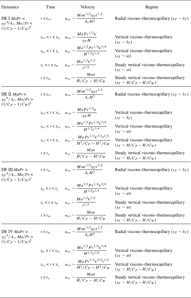
Based on the comparison between different time scales, it may be demonstrated that there exist four possible dynamical evolutions. Further, the scaling law has been summarised in table 1 under different regimes in four possible dynamical evolutions.
Scaling laws of the surface flow.

For further understanding, figure 2 shows the distribution of four possible dynamical evolutions in the C W –Pr–Ma parameter space.
Figure 3 shows regimes of the surface flow in various dynamical evolution regimes. The distinct stages may be dominated under the radial viscous–thermocapillary (x
T
∼ δ
T
) (RK), vertical viscous–thermocapillary (x
T
∼ δ
T
) (VK), vertical viscous–thermocapillary (x
T
∼ ut) (VC), steady vertical viscous–thermocapillary (x
T
∼ ut) (SVC) and steady vertical viscous–thermocapillary (x
T
∼
 $ H /{C_{P}} $
–
 $ H / {C_{W}} $
) (SVCS) regimes in the dynamical evolution DE I, under the RK, VK, VC, vertical viscous–thermocapillary (VCS) and SVCS regimes in the dynamical evolution DE II, under the RK, VC, SVC and SVCS regimes in the dynamical evolution DE III and under the RK, VC, VCS and SVCS regimes in the dynamical evolution DE IV, respectively.
Figure 4 shows different velocity scaling laws in different stages of the surface flow in two typical scenarios of the dynamical evolution. In the dynamical evolution DE I, the surface velocity may be scaled by (3.9) in the first stage, remain a constant value and be scaled by (3.12) in the second stage, decrease and be scaled by (3.11) in the third stage, decrease further and be scaled by (3.15) in the fourth stage and finally remain a constant value again and be scaled by (3.17) in the fifth stage, as shown in figure 4(a). Additionally, in the dynamical evolution DE IV, the surface velocity may be scaled by (3.9) in the first stage, decrease and be scaled by (3.11) in the second stage, increase again and be scaled by (3.18) in the third stage and remain a constant value again and be scaled by (3.17) in the fourth stage, as shown in figure 4(b).
Distribution of four possible dynamical evolution s in the C
W
–Pr–Ma space. Here, the surface S1 is MaPr = η
T
4
 $ / $
 $ A_{\varepsilon} $
, and the surface S2 is Ma
 $ / $
Pr = (
 $ 1/{C_{P}} $
–
 $ 1/{C_{W}} $
)2.

Regimes of surface flow in different dynamical evolutions.

Velocities of surface flow in two typical dynamical evolutions for C
W
= 20. Here, in DE I for Ma = 150, t
s
= t
ss
in (a), given by (3.16) for MaPr < η
T
4
 $ / $
 $ A_{\varepsilon} $
and
 $ \textit{Ma}/\textit{Pr} $
< (
 $ 1/{C_{P}} $
–
 $ 1/{C_{W}} $
)2, but in DE IV for Ma = 50 000, t
s
= t
ν
in (b), given by (3.5) for MaPr > η
T
4
 $ / $
 $ A_{\varepsilon} $
and
 $ \textit{Ma}/\textit{Pr} $
> (
 $ 1/{C_{P}} $
–
 $ 1/{C_{W}} $
)2.

3.3. Steady vertical flow
The surface flow drives the fluid away from the heated wire, causing a drop of radial pressure near the wire. Consequently, a balance between the pressure gradient and the thermocapillary force can be established in (2.2). Integrating (2.2) vertically yields
 \begin{align} \frac{{\unicode[Arial]{x0394}} p}{\rho \delta _{p}}\delta _{\nu }\sim \frac{\textit{MaPr}\kappa ^{2}}{Hx_{T}}, \end{align}
where, δ
p
represents a thickness in the radial direction for a vertical flow near the wire, across which the greatest pressure change occurs. This pressure drop (
 $ \Delta $
p ∼ MaPrκ
2
δ
p
 $ / $
(Hx
T
δ
ν
)) can generate a pressure gradient in the vertical direction, which subsequently drives the vertical flow near the wire to maintain continuity. Furthermore, the penetration distance of the vertical flow may be estimated by vt when t <
 $ H/v $
but by H when t ≥
 $ H/v $
. As the vertical flow is sourced from the surface flow, their volumetric flow rates are identical
 \begin{align} Q\sim u\delta _{\nu }2\pi x_{T}\sim v\left(\left(\delta _{p}+H/C_{W}\right)^{2}-H^{2}/{C_{W}}^{2}\right)\pi . \end{align}
As described in § 3.2, the velocity varies for the surface flow across different regimes under different dynamical evolutions. Since the vertical flow is driven by the vertical pressure gradient induced by the surface flow, the dynamical evolution in the vertical flow is dependent on those in the surface flow, as described in table 1, and appears extremely complex. Accordingly, we performed a simple scaling analysis only for the steady vertical flow for simplification and validation.
Clearly, the maximum penetration depth is H and x
T
becomes the constant length
 $ H /{C_{P}} $
–
 $ H / {C_{W}} $
for the vertical flow in the vt ≥ H and δ
ν
∼ H steady stage. Substituting the pressure drop (3.19) into (2.3), the balance between vertical pressure gradient and viscous terms may be expressed as
 \begin{align} \frac{1}{\rho }\frac{\partial p}{\partial z}\sim \frac{{\unicode[Arial]{x0394}} p}{\rho H}\sim \frac{\textit{MaPr}\kappa ^{2}\delta _{p}}{H^{4}/C_{P}-H^{4}/C_{W}}\sim \textit{Pr}\kappa \frac{v}{\delta _{p}^{2}}. \end{align}
The volumetric flow rate of the surface flow may be given by
 \begin{align} Q_{s}\sim u_{ss}H\sim \frac{Ma\kappa }{1/C_{P}-1/C_{W}}. \end{align}
Further, based on (3.20), (3.21) and (3.22), the velocity of the steady vertical flow is scaled by
 \begin{align} v_{s}\sim \frac{8^{1/5}Ma\kappa }{\left(1/C_{P}-1/C_{W}\right)^{2/5}H}. \end{align}
Additionally, the analysis can be extended to re-examine the vertical thermal boundary layer around the vertical wire in the steady state. The unsteady and convection terms in (2.4) may be characterised by O(
 $ T/t $
) and O(
 $ vT/H $
). Thus, the time scale at which these two terms become equivalent is formulated as
 \begin{align} t_{\kappa }\sim \frac{H^{2}/C_{P}-H^{2}/C_{W}}{\textit{Ma}\kappa }. \end{align}
This means that t
κ
 $ T/ $
t
ss
∼ 1
 $ T/ $
(
 $ 1/{C_{P}} $
–
 $ 1/{C_{W}} $
) < 1. In other words, in the steady state, heat transfer is governed by a balance between convection and conduction in the thermal boundary layer.
The thermal boundary layer ceases to thicken and the thickness becomes a constant value δ
Ts
in the steady state for which convection balances conduction. Integrating (2.4) in the r-direction from
 $ H / {C_{W}} $
to
 $ H / {C_{W}} $
+ δ
Ts
yields a relationship
 \begin{align} \int _{H/C_{W}}^{H/C_{W}+\delta _{Ts}}v\frac{\partial T}{\partial z}r{\rm d}r\sim \int _{H/C_{W}}^{H/C_{W}+\delta _{Ts}}\kappa \frac{\partial }{\partial r}\left(r\frac{\partial T}{\partial r}\right){\rm d}r. \end{align}
Consequently, such an implicit relationship between δ
Ts
and
 $ v $
s
may be given by
 \begin{align} v_{s}\sim \frac{2\kappa }{H\eta _{Ts}}. \end{align}
Here, the factor of the curvature in the steady stage (η Ts ) is defined as
 \begin{align} \eta _{Ts}\sim C_{W}\frac{{\delta _{Ts}}^{3}}{H^{3}}+2\frac{{\delta _{Ts}}^{2}}{H^{2}}. \end{align}
Incorporating (3.23) and (3.26), a balance between the thermocapillary and viscous terms in (3.7) yields such a scale
 \begin{align} \eta _{Ts}\sim \frac{\left(2/C_{P}-2/C_{W}\right)^{2/5}}{\textit{Ma}}. \end{align}
We may combine (3.27) and (3.28), and the derivative of δ Ts with respect to C W can be expressed as
 \begin{align} \frac{\partial \delta _{Ts}}{\partial C_{W}}\sim \frac{4/\left(5\textit{Ma}{C_{W}}^{2}\left(2/C_{P}- 2/C_{W}\right)^{3/5}\right)-{\delta _{Ts}}^{3}/H^{3}}{3C_{W}{\delta _{Ts}}^{2}/H^{3}+ 4\delta _{Ts}/H^{2}}. \end{align}
Note that the thermal boundary layer becomes thin as the wire’s curvature C
W
increases for ∂δ
Ts
 $ T/ $
∂C
W
< 0, which is negative in the current range of parameters in this study.
Heat transfer from the wire may be estimated as O(λ
 $ \Delta $
T
 $ / $
δ
T
), with λ denoting the thermal conductivity. Accordingly, the heat flux can be non-dimensionalised by
 $ \lambda\Delta T $
 $ /H $
and the Nusselt number in the steady stage (Nu
s
) can be derived based on (3.28)
 \begin{align} \textit{Nu}_{s}\sim \frac{Ma^{1/2}{\delta _{\textit{Ts}}}^{1/2}{C_{W}}^{1/2}}{H^{1/2}}. \end{align}
4. Numerical method
Two-dimensional axisymmetric numerical simulations are employed to characterise transient thermocapillary convection flows (Villers & Platten Reference Villers and Platten1992). For simplicity, the governing equations, (2.1)–(2.4), may be non-dimensionalised using the following reference scales: the length by H, velocity by Maκ
 $ / $
H, time by H
2
 $ / $
(Maκ), pressure by ρMa
2
κ
2
 $ / $
H
2and temperature difference by
 $ \Delta T $
. The dimensionless variables (denoted with an asterisk) are thus defined as: r
* = r
 $ / $
H, z
* = z
 $ / $
H,
 $ \varepsilon $
* =
 $ \varepsilon $
 $ / $
H and δ
* = δ
 $ / $
H (radial and axial coordinates normalised by H), t
* = t
 $ / $
(H
2
 $ / $
(Maκ)), u
* = u
 $ / $
(Maκ
 $ / $
H),
 $ v $
* =
 $ v $
 $ / $
(Maκ
 $ / $
H), p
* = p
 $ / $
(ρMa
2
κ
2
 $ / $
H
2) and T
* = (T − T
0)
 $ / $
 $ \Delta T $
(also see Kamotani, Ostrach & Masud Reference Kamotani, Ostrach and Masud2000).
Schematic of boundary conditions and computational domain.

Figure 5 shows the numerical computation model, where the dashed-line box involves the 2-D axisymmetric computational domain. The fluid within the domain is initially isothermal at a temperature of zero and motionless. Boundary conditions are assumed as
 \begin{align} u^{*} & = v^{*} = 0\ \text{at}\ r^{*}=1/C_{W}, 1/C_{P}\ \text{and}\ z^{*}=0; \nonumber\\ v^{*} &= 0\ {\textrm{at}}\ z^{*}=1; \nonumber\\ T^{*} &= 1\ {\textrm{at}}\ r^{*}={\textrm{1}}/C_{W}; \nonumber\\ T^{*} &= 0\ {\textrm{at}}\ r^{*}={\textrm{1}}/C_{P}; \nonumber\\ \dfrac{\partial T^{*}}{\partial z^{*}} & = 0\text{ at }z^{*}=0,1. \end{align}
The surface boundary is imposed by a Marangoni stress, which is expressed as
 \begin{align} \frac{\partial u^{*}}{\partial z^{*}}=\frac{\partial T^{*}}{\partial r^{*}}\text{at }\,z^{*}=1. \end{align}
The analysis that follows is based on the assumption that the surface is flat, as indicated by Popinet (Reference Popinet2018). Here, the computational domain is considered as a cylindrical pool in which the side boundary is a sidewall. The previous studies (Li, Zhang & Zhang Reference Li, Zhang and Zhang2019; Meng et al. Reference Meng, Chen and Xu2024b ) have also demonstrated that thermocapillary convection flows can be effectively characterised through numerical simulations incorporating Marangoni stress on a flat surface.
In this study, the governing equations, (2.1)–(2.4), were numerically solved using ANSYS Fluent 16.0 for which a finite volume method was employed with a pressure-based solver. Further, the Semi-Implicit Method for Pressure Linked Equations was adopted for pressure–velocity coupling where the gradient term was discretised with the Green–Gauss node-based scheme, the pressure term with the second-order scheme, the advection term in the momentum equations with the Quadratic Upstream Interpolation for Convective Kinematics but in the energy equation with the second-order upwind scheme and the time term with the second-order backward Euler implicit scheme (see Zeng et al. Reference Zeng, Mizuseki, Simamura, Fukuda, Higashino and Kawazoe2001; Mo et al. Reference Mo, Zhang, Ruan and Li2021).
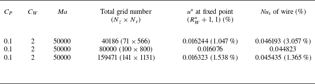
A mesh sensitivity analysis was conducted using three non-uniform (geometrically stretched) mesh configurations, with finer cells in the regions adjacent to the surface and thermal boundaries. The horizontal expansion of the computational cells follows a constant growth rate from the sizes of 0.006, 0.0025 and 0.002 (adjacent to wire) to the sizes of 0.012, 0.01 and 0.006, respectively. Similarly, the cells grow vertically from the sizes of 0.01, 0.008 and 0.005 (surface) to the sizes of 0.018, 0.012 and 0.01 (bottom), respectively. We performed the mesh sensitivity test for the smallest non-dimensional curvature of C
W
= 2 and the Marangoni number of Ma = 50 000. The velocity at the monitor point (
 $ R_{W}^{*} $
+ 1, 1) and Nusselt number are presented in table 2, where N
r
and N
z
are the numbers of cells in the radial and vertical directions. We employed the mesh of 100 × 800 under consideration of computing cost and numerical accuracy in this study.
Mesh dependency test.

Notes: Percentage (%) denotes the relative difference in comparison with the other case, and the total grid number is the production of vertical number (N z ) and radial number (N r ).
The results from the current computational procedures were additionally validated against experimental results in Kang et al. (Reference Kang, Wu, Duan, He, Hu, Duan and Hu2019). Figure 6 shows the profile of the temperature on the surface of the liquid in the annular pool. Numerical results are consistent with experimental results in Kang et al. (Reference Kang, Wu, Duan, He, Hu, Duan and Hu2019) with an acceptable mean error of 3.88 %. The discrepancy between numerical and experimental results is because the conditions of the background and boundary of the annular pool in the experiment are not perfectly isothermal like those in numerical simulation. That is, the current numerical procedures may be applied for thermocapillary convection flows in the annular pool.
Temperature profiles at z * = 1 for Ma = 1.15 × 10⁵, C W = 0.25 and Pr = 20 where experimental results are obtained from Kang et al. (Reference Kang, Wu, Duan, He, Hu, Duan and Hu2019).

5. Numerical results and validations
To characterise transient flows across various regimes and to validate the scaling laws proposed in § 3, a 2-D axisymmetric numerical simulation was performed for a fixed pool curvature of C P = 0.1 and Prandtl number of Pr = 100 (representative of silicone oils of order 10 cSt) but C W from 2 to 1000 and Ma from 150 to 50 000, which may encompass all regimes.
5.1. Characteristics of thermocapillary convection flows
Figure 7 presents a couple of typical flows in two different scenarios. Thermocapillary convection flows at t
∗
 $ / t_{\textit{ss}}^{*} $
= 10−7 for MaPr < η
T
4
 $ / $
 $ A_{\varepsilon} $
and
 $ \textit{Ma}/\textit{Pr} $
< (
 $ 1/{C_{P}} $
–
 $ 1/{C_{W}} $
)2 under the RK regime in the dynamical evolution DE I (see table 1) are shown in figure 7(a). Clearly, the isotherms are substantially parallel with the spacing between neighbouring isotherms increasing away from the heated wire due the curvature effect. This implies that thermocapillary convection flows are weak and conduction is dominant. Figure 7(b) shows isotherms at t
∗
 $ /t_{\textit{ss}}^{*} $
= 10−5 for MaPr > η
T
4
 $ / $
 $ A_{\varepsilon} $
and
 $ \textit{Ma}/\textit{Pr} $
< (
 $ 1/{C_{P}} $
–
 $ 1/{C_{W}} $
)2 under the VC regime in the dynamical evolution DE III. Clearly, the thermal boundary layer becomes thinner and the isotherms are contorted. This is because strong convective flows occur for which the strong surface flow travels away from the heated wire.
Isotherms from 0.05 to 0.95 with an interval between two neighbouring isotherms being 0.05 for Pr = 100. Panels show (a) Ma = 150 and C W = 2 under RK regime in DE I and (b) Ma = 5000 and C W = 2 under VC regime in DE III.

Figure 8 shows isotherms and streamlines in a steady state. For a smaller Ma in DE I, the surface tension is small, and heat transfer in the liquid pool is dominated by conduction. As shown in figure 8(a,c,e), the thermal diffusion in the radial direction near the heated wire is significant, resulting in denser isotherms, and the variance of the wire curvature may change the temperature distribution. In particular, as the distance from the wire increases, the thermal diffusion becomes smaller with sparser isotherms due to the curvature effect. Further, as the curvature radius increases, the thermal diffusion becomes stronger, for which the same isotherm is further from the wire, as shown in figure 8(a,c,e). This trend is consistent with the monotonicity analysis of (3.29), which indicates that a larger curvature leads to a thinner thermal boundary layer. Figure 8(g) also shows streamlines and isotherms in the rectangular pool for comparison. Additionally, since conduction is dominant, convection is weak and there exists only one circulation in the pool, which moves away from the wire as the wire radius increases.
Streamlines and isotherms from 0.05 to 0.95 with an interval between two neighbouring isotherms being 0.05 at steady state under SVCS regime for Pr = 100. Panels show (a) Ma = 150 and C W = 1000 in DE I; (b) Ma = 5000 and C W = 1000 in DE III; (c) Ma = 150 and C W = 20 in DE I; (d) Ma = 5000 and C W = 20 in DE III; (e) Ma = 150 and C W = 2 in DE I; (f) Ma = 5000 and C W = 2 in DE III; (g) Ma = 150 in rectangular pool; (h) Ma = 5000 in rectangular pool.

Thermal boundary layer thickness under RK regime in dynamical evolutions DE I–DE IV for Ma = 150, 500 and 5000. The fitting line (t
* <
 $ t_{\kappa}^{*} $
) has a slope of a = 1.82090 and an intercept of b = 0.04193. The 95 % confidence interval for this fitting line is [1.76542, 1.87639] (for the slope) and [0.00465, 0.07931] (for the intercept).

For a larger Ma in DE III, the thermal boundary layer is distinct and the surface flow becomes much stronger with more circulations, as shown in figure 8(b,d,f). The examination of numerical results shows that convection becomes stronger as the wire radius increases. Here, streamlines and isotherms in the rectangular cavity are also plotted in figure 8(h) for comparison.
5.2. Validation of selected scaling laws
Scaling analysis shows that, once a vertical wire is suddenly heated, heat transfer occurs, resulting in an appearance and development of a thermal boundary layer around the vertical wire, which may be scaled by (3.2). The thermal boundary layer thickness was measured from numerical results, defined as the length from the wire’s surface to the isotherm of T
* = 0.1 at z
* = 0.2. Figure 9 shows the dependence with time of the thermal boundary layer thickness under conduction dominance for different curvatures and Marangoni numbers. The fitting line is obtained using the least-squares linear regression and the 95 % confidence intervals are determined by the standard error of the estimate. Using this linear regression approach, we derived the proportionality coefficient (i.e. slope, a) and offset (i.e. intercept, b). The method is consistently applied to each subsequent figure. A linear relation between
 $ \delta_{T}^{*} $
Ma
 $ ^{1/2} $
and κ
 $ ^{1/2} $
t
 $ ^{1/2} $
η
T
, where the scaling laws (3.2) and (3.3) are presented in a non-dimensional format, is good, implying that the prediction by the scaling laws (3.2) and (3.3) is consistent with numerical results. The scaling laws (3.2) and (3.3) may be used to quantify the development of the thermal boundary layer around the vertical wire with time after sudden heating.
According to the analysis in § 3, the thermocapillary force, which arises from the non-uniform temperature distribution following sudden heating, is capable of driving a surface flow. The surface flow velocity may be described by (3.17). For validation, the velocity was extracted for the isotherm of T
∗ = 0.3 at z
* = 1. Figure 10 shows the relationship between
 $ u_{\textit{ss}}^{*} $
Maκ
 $ / $
H and Maκ
 $ / $
(
 $ H /{C_{P}} $
–
 $ H / {C_{W}} $
) in the steady stage under the SVCS regime in dynamical evolutions DE I–DE IV. Note that the dimensional velocity
 $ u_{\textit{ss}}^{*} $
Maκ
 $ / $
H is here adopted for easy observation. The dimensional velocity has an approximately linear relation with Maκ
 $ / $
(
 $ H /{C_{P}} $
–
 $ H / {C_{W}} $
), thereby confirming the validity of the scaling law presented in (3.17).
Surface flow velocity in steady stage under SVCS regime in dynamical evolutions DE I–DE IV. The fitting line has a slope of a = 0.43693 and an intercept of b = −3.40611 × 10⁻⁴. The 95 % confidence interval for this fitting line is [0.39637, 0.47646] (for the slope) and [−0.00815, 0.00747] (for the intercept).

As described above, a vertical flow is driven by a vertical pressure gradient induced by a surface flow. In numerical results, the vertical flow velocity is defined as the maximum velocity at z
∗ = 0.5. Figure 11 presents the velocity in the steady stage under the SVCS regime in dynamical evolutions DE I–DE IV extracted from numerical results. Clearly, the dimensional velocity
 $ v_{s}^{*} $
Maκ
 $ / $
H in (3.23) has a linear relation with 8
 $ ^{1/5} $
Maκ
 $ / $
H(
 $ 1/{C_{P}} $
–
 $ 1/{C_{W}} $
)
 $ ^{2/5} $
, which confirms that the prediction by (3.23) may describe the vertical flow in the steady state under the SVCS regime.
Vertical flow velocity in steady stage under SVCS regime in dynamical evolutions DE I–DE IV. The fitting line has a slope of a = 0.01175 and an intercept of b = 0.00117. The 95 % confidence interval for this fitting line is [0.01026, 0.01323] (for the slope) and [−7.43458 × 10⁻⁴, 0.00309] (for the intercept).

In the fully developed stage, the thermal boundary layer ceases to thicken further. Heat transfer is governed by a balance between conduction and convection, which leads to a relationship between
 $ v $
s
and η
Ts
given by (3.26). The corresponding numerical results are shown in figure 12 under the SVCS regime in dynamical evolutions DE I–DE IV. It is seen from this figure that
 $ v_{s}^{*} $
Ma has an approximately linear relation with η
Ts
, which confirms the scaling law (3.26).
Surface flow velocity in steady stage under SVCS regime in dynamical evolutions DE I–DE IV. The fitting line has a slope of a = 0.70561 and an intercept of b = 6.45031. The 95 % confidence interval for this fitting line is [0.59668, 0.81461] (for the slope) and [3.00185, 9.89878] (for the intercept).

Scaling analysis indicates that the thermal boundary layer thickness δ
Ts
has an implicit relation with the curvature factor in the steady state η
Ts
, as described in (3.28). Further, the curvature factor in the steady state may also be expressed by the curvature of the wire and cylinder pool in (3.28). Figure 13 shows the dependence of η
Ts
on (
 $ 1/{C_{P}} $
–
 $ 1/{C_{W}} $
)
 $ ^{2/5} $
 $ / $
Ma from numerical results. There is a good linear correlation between η
Ts
and (
 $ 1/{C_{P}} $
–
 $ 1/{C_{W}} $
)
 $ ^{2/5} $
 $ / $
Ma, suggesting that (3.28) is able to predict the thermal boundary layer thickness in the steady state.
Curvature factor in steady stage under SVCS regime in dynamical evolutions DE I–DE IV. The fitting line has a slope of a = 0.00548 and an intercept of b = 0.11369. The 95 % confidence interval for this fitting line is [0.00320, 0.00776] (for the slope) and [−0.10735, 0.33472] (for the intercept).

The flow around the wire may be quantified by the flow rate Q
s
, which is scaled by (3.22). To verify (3.22), the volumetric flow rates in the steady stage were calculated from numerical results in dynamical regimes DE I–DE IV. Figure 14 shows the flow rate for different curvatures. Similar to figure 10, the dimensional volumetric flow rate
 $ Q_{s}^{*} $
Maκ is here adopted for easy observation. Clearly, the dimensional volumetric flow rate
 $ Q_{s}^{*} $
Maκ has a linear relation with Maκ
 $ / $
(
 $ 1/{C_{P}} $
–
 $ 1/{C_{W}} $
), which also validates the scaling law (3.22).
Volumetric flow rate in steady stage under SVCS regime in dynamical evolutions DE I–DE IV. The fitting line has a slope of a = 0.18515 and an intercept of b = 4.31787 × 10⁻⁷. The 95 % confidence interval for this fitting line is [0.11738, 0.21292] (for the slope) and [−1.11067 × 10⁻⁶, 1.97428 × 10⁻⁶] (for the intercept).

The Nusselt number Nu
s
, which characterises heat transfer in the steady stage, is scaled by (3.30). For the validity of (3.30), the Nusselt number was calculated in dynamical evolutions DE I–DE IV using numerical results. As illustrated in figure 15, a good linear relationship may be observed between Nu
s
and Ma
 $ ^{1/2} $
 $ \delta_{\textit{Ts}}^{*} $
 $ ^{1/2} $
C
W
 $ ^{1/2} $
in the steady stage. This means that the scaling prediction of (3.30) is consistent with numerical results. The further error analysis also indicates that the linear regression coefficient achieves R
2 = 0.9210, exceeding the empirical threshold of R
2 > 0.9 (Xue et al. Reference Xue, Zhao, Zhang and Cheng2023), suggesting that the scaling law (3.30) is validated.
Nusselt number in steady stage under SVCS regime in dynamical evolutions DE I–DE IV. The fitting line has a slope of a = 0.52686 and an intercept of b = 7.74745. The 95 % confidence interval for this fitting line is [0.43625, 0.61506] (for the slope) and [−2.66026, 18.15516] (for the intercept).

6. Conclusions
Transient thermocapillary convection flows near a suddenly heated wire are investigated through scaling analysis and axisymmetric numerical simulation. These flows exhibit unique dynamical and thermal behaviours that distinguish them from those adjacent to a flat wall. For sudden heating, heat is conducted from the wire into the surrounding liquid and forms an annular, vertical thermal boundary layer of thickness δ T . The resulting radial temperature gradient may generate a thermocapillary force on the surface of the liquid that drives liquid radially away from the wire. In different regimes, the thermocapillary force may be balanced either by radial or by vertical viscous diffusion. Further, such a surface flow induces a vertical pressure gradient along the wire, which drives a vertical flow around the wire. Finally, a steady state is reached when the heat conducted from the wire is equal to that convected away. In this study, the thermal boundary layer, surface flow and vertical flow around the vertical wire are described by different scaling laws dependent on the wire curvature C W , Marangoni number Ma and Prandtl number Pr.
The curvature effects can be described by the curvature factors η
T
and η
Ts
for transient and steady thermal boundary layers, respectively. The transient thermal boundary layer is under an unsteady–conduction balance, with the thickness being κ
 $ ^{1/2} $
t
 $ ^{1/2} $
η
T
, and the steady thermal boundary layer is under convection–conduction balance, with a relationship of η
Ts
∼ (2
 $ / $
C
P
– 2
 $ / $
C
W
)
 $ ^{2/5} $
 $ / $
Ma. The surface flow has four dynamical evolutions within the parameter space, encompassing six regimes. For instance, in a typical dynamical evolution DE I, a surface flow may be dominated under the radial viscous–thermocapillary (x
T
∼ δ
T
), vertical viscous–thermocapillary (x
T
∼ δ
T
), vertical viscous–thermocapillary (x
T
∼ ut), steady vertical viscous–thermocapillary (x
T
∼ ut) and steady vertical viscous–thermocapillary (x
T
∼
 $ H /{C_{P}} $
–
 $ H / {C_{W}} $
) regimes. Additionally, the vertical flow velocity and heat transfer in the steady state have been scaled.
Further, the 2-D axisymmetric numerical simulations were conducted to analyse transient flows and to verify the representative scaling laws. The velocity and thickness of the surface and vertical flows as well as the Nusselt number have been calculated, and show good agreement with the scaling predictions. This means that the scaling laws obtained in this study can be employed to characterise transient thermocapillary convection flows around the suddenly heated wire, which further deliver actionable guidance for controlling transient fluid flows in thermal-probe microscopes and establish a foundation for advancing crystal-manufacturing techniques.
Funding
We thank the National Natural Science Foundation of China (12302349) for financial support. We also appreciate the technical support provided by Space Application System of China Manned Space Program.
Declaration of interests
The authors report no conflict of interest.