Introduction
In the present day warfield, most radars such as reconnaissance, surveillance, and target tracking radars, have to deal with very capable and advanced threats that are designed to contribute to the deterioration of radar operations. Electronic attack (EA) systems, electronic warfare support (ES), anti-radiation missiles (ARMs) and radar warning receivers are examples of such a threat. Therefore, radars are required to be invisible and hence are called low probability of intercept (LPI) radars. To make the necessary detection, tracking and at the same time hide from enemy attacks, radar systems should be LPI [Reference Alrubeaan, Albagami, Ragheb, Aldosari, Altamimi and Alshebeili1, Reference Kishore and DeerghaRao2]. LPI radars have many advantages such as wide bandwidth, low transmit power, high resolution, and low cost. LPI radars use special design features that make it difficult to be detected by the passive receivers such as Electronic Intelligence (ELINT) receivers [Reference Vanhoy, Schucker and Bose3]. In addition to the difficulty of finding it, LPI radar offers other benefits that include finding higher resolution solutions for short-term applications, lower costs, and low power compared to solid-state structures. Since LPI radars use low transmit power, the probability of being damaged by precise guided munitions and ARMs is also very less. LPI radars can detect the targets at long distances compared to intercept receivers. For ELINT systems, it is important to distinguish intrapulse waveforms after signal acquisition [Reference Phillip4, Reference Taboada, Lima, Gau, Jarp and Pace5]. Linear frequency modulation (LFM), nonlinear frequency modulation, Barker, polytime codes, and polyphase codes including Frank codes are some of the LPI waveforms which are difficult to intercept and analyze. These signals are used in a variety of sensitive EW devices like EAs, electronic support, and radar emitter detection.
The success of an LPI radar depends on the type and length of the waveform used [Reference Chilukuri, Kakarla and Subbarao6]. The modern intercept receivers should perform the functions of detecting, estimating, and classifying LPI signals even when the received signal is contaminated with noise [Reference Shyam sunder7]. Since the signals are LPI signals, it is difficult for the electronic receivers to intercept the target. In recent years, the significance of intrapulse modulation of LPI radars is increased heavily in the area of multi-input multi-output (MIMO) radars and EW systems. Precise measurement of intrapulse parameters and the knowledge of the type of the waveform will provide the information about the threat to the radar so that the EA or ES system could take instantaneous counter action against the enemy. The knowledge of the parameters will also help to develop smart receivers which can intercept, detect, and analyze the waveforms [Reference Stephens8]. Identification of parameters also facilitates to reguide and to re-transmit without impact on the electronic system. The parameters also help in the development of systems such as MIMO radar, ES, and EA systems [Reference Singh and Subba Rao9, Reference Ma, Huang, Lin and Huang10]. In addition, the parameters also help to distinguish duo radars operating at very close frequencies. It also provides information regarding the type of waveform used which is essential to develop intercept receivers. Normally, the received signal is corrupted with various types of noises and the detection or measurement efficiency decreases very badly [Reference Alrubeaan, Albagami, Ragheb, Aldosari, Altamimi and Alshebeili1, Reference Kishore and DeerghaRao2, Reference Ma, Huang, Lin and Huang10]. Two main sources of noise are
(i) Thermal noise introduced by the electronic devices.
(ii) Generally, the receivers are placed at a long distance from the control and command center. The channel or the medium through which the radar signals transmit increases the noise further.
To improve the detection and measurement accuracy, the noisy signal should be preprocessed first using denoising algorithms. In [Reference Shyam sunder7], modified S-transform (MST) algorithm is used to estimate the parameters of polyphase codes which are corrupted with noise. Since the MST algorithm provides good time-frequency (TF) isolation property, it is found to be effective even in a noisy environment [Reference Biswal, Dash and Biswal11]. To analyze noisy signals, the MST coefficients are computed first. Later post-processing technique based on power threshold method is used to estimate the parameters. A threshold value for power was setup. If the MST coefficient is less than the threshold value, it is considered as noise and the coefficient is made zero. With a threshold value of 0.7, the parameters are estimated with an accuracy of >95% up to −6 dB signal-to-noise ratio (SNR).
In [Reference Chilukuri, Kakarla and Subbarao6], polytime coded waveforms using cyclostationary (CS) algorithm are analyzed with the assumption that the received signal is free from noise. The parameters extracted are bandwidth, carrier frequency, and code rate. All the parameters are estimated with an error of <5% when the sampling frequency is ≥5 times the carrier frequency. In [Reference Alrubeaan, Albagami, Ragheb, Aldosari, Altamimi and Alshebeili1], the authors have extracted the features and classified the LPI signals using Wigner distribution and radon transform. The percentage of classification is better than 87 for all polyphase codes except P 3 when the SNR is −2 dB or high. In [Reference Kishore and DeerghaRao2], the authors have classified various types of LPI radar waveforms using feature extraction based on radon ambiguity transform and radon-Wigner-Ville distribution. The classification is better than 95% for LFM and polyphase modulations up to −10 dB SNR. In [Reference Ma, Huang, Lin and Huang10], the authors have classified 11 types of LPI radar waveforms under various noise conditions and achieved an overall recognition rate of 87.7% when the SNR is −6 dB or high. Singh and coworkers estimated the intrapulse modulation parameters using all phase FFT algorithm and the same is implemented on a high-speed FPGA-based digital receiver.
Although, several research papers are available on the classification of modulation waveforms, very little work is done on the estimation of modulation parameters. In this paper, polyphase and polytime coded waveforms of LPI radar in the presence of noise are analyzed using CS techniques and estimated the modulation parameters. To improve the signal quality, two types of denoising filters are used. In section “CS algorithm”, CS techniques are discussed. Basic equations for the generation of polyphase and polytime codes are given in section “Polyphase and polytime codes”. Denoising techniques to improve the signal quality are briefly discussed in section “Denoising techniques”. The analysis of LPI radar waveforms and the simulation results are discussed in section “Analysis of intrapulse modulated waveforms”. Generation and complete analysis of the waveforms are carried out in MATLAB.
CS algorithm
Nonstationary signals are efficiently analyzed using TF algorithms which can analyze the signals in both the domains simultaneously. Many TF methods are available in the literature [Reference Chilukuri, Kakarla and Subbarao6, Reference Biswal, Dash and Biswal11–Reference Bouillaut and Sidahmed14]. CS algorithm is used here to estimate the modulation parameters. This algorithm is more suitable for the analysis of periodic signals like LPI waveforms. In CS method, the signal is converted into cycle frequency – frequency plane or bi-frequency plane [Reference Prithivi Raj, Saran Kumar, Kalaiyarasan, Praveen Chandru and Nandakumar Singh15]. CS method offers some properties which cannot be obtained from other TF methods. Cyclic autocorrelation function (CACF) and spectral correlation density (SCD) are the key parameters in CS analysis. In frequency domain, the statistical behavior of the signal is completely described by the SCD function. CS techniques are widely used in many areas such as estimation of parameters, array processing, detection of signals, estimation of direction, and time of arrival and parameter extraction. Many characteristics of LPI radar are estimated using CS algorithm by calculating CACF and the SCD coefficients [Reference Chilukuri, Kakarla and Subbarao6, Reference Gardner16, Reference Lima17].
Let x(t) be the signal to be analyzed. The auto correlation function of x(t) is computed using equation (1) and its CACF is calculated using equation (2)


where α represents cycle frequency. The power spectrum of the signal is computed using equation (3)

and the SCD coefficients are computed using equation (4)


Equation (5) is the Fourier transform of x(v). $\;\;S_x^\alpha ( f ) \;$ represents the bi-frequency plane or (f, α) plane. Since the signals being analyzed are defined over a finite time interval T, the SCD coefficients of a finite length signal are estimated using equation (6). The SCD is a function of two parameters – time and frequency.


and $T_W^{}$ is the short-time FFT window length.
Equations (9) and (10) represent the discrete equivalent of equations (6) and (8) respectively and the SCD coefficients of the waveforms are computed as given in equation (9)


Equation (10) is the N-point FFT of x(n), N is the number of points and W(n) is the window. The discrete equivalent of α is represented by γ. Assuming that the sampling frequency is represented by f s,


and M is selected such that f s/M >>1. Figure 1 shows the block diagram to compute the SCD coefficients using direct frequency smoothing (DFS) method.
Computation of SCD values using DFS method.

Polyphase and polytime codes
Polyphase codes
Polyphase codes (Frank and P 1, P 2, P 3, P 4) are obtained from LFM waveform or stepped frequency waveform [Reference Alrubeaan, Albagami, Ragheb, Aldosari, Altamimi and Alshebeili1, Reference Shyam Sunder and Subbarao12, Reference Vellanki and Satish Babu18, Reference Skolnik19]. The polyphase codes are generated using equations (13–17).
Frank code
Frank code is generated from a step or LFM waveform using M frequency steps and M samples per frequency using equation (13). The number of subcodes or phases is given by N C = M 2.

P 1 code
The number of subcodes or phases for P 1 code is same as for Frank code ( i.e. N C = M 2). P 1 code is generated using equation (14).

P 2 code
In P 2 code, M should be even, and code length is N C = M 2. P 2 code is generated using equation (15).

P 3 code
The phase for the k th sample is shown in equation (16) where k = 1, 2, …, N c.

P 4 code
The phase for the k th sample is shown by equation (17) where k = 1, 2, …, N c.

Polytime codes
Four types of polytime codes are used. They are denoted as T 1(n), T 2(n), T 3(n), and T 4(n). The wrapped phases of the polytime codes are generated using equations (18–21). Here the number of phase states are assumed to be n = 2 (0° and 180°).
T 1(n) code
T 1(n) code is generated from the stepped frequency waveform using equation (18).

k is the number of segments and T is the duration of the code [Reference Chilukuri, Kakarla and Subbarao6, Reference Fielding20].
T 2(n) code
The T 2(n) code is generated using equation (19).

T 3(n) code
T 3(n) code is generated using equation (20).

where ΔF represents the modulation bandwidth.
T 4(n) code
T 4(n) code is generated using equation (21).

where INT[..] is the integer part, MOD[..] is the reminder function and all the other variables are defined as above.
Denoising techniques
In any measurement, noise is inevitable and the signal is corrupted with noise and device intrinsic. By pre-processing the signal using denoising algorithms, the measurement accuracy could be improved greatly. The filters generally used to denoise the signals are Golay filter, Savitzky-Golay (SG) filter, moving average filter, mean filter, median filter, wavelet filters, and MST. To assess the performance of the denoising algorithm, SNR is used as a figure of merit. In this work, SG filter and median filter are used to improve the SNR [Reference Ma, Huang, Lin and Huang10, Reference Biswal, Dash and Biswal11, Reference Dombi and Dineva21–Reference Siva Sankara Reddy and Thirumala Rao24].
SG filter
SG filter is a data smoothing filter based on local least squares polynomial approximation. This method reduces the noise while maintaining the shape and height of the waveform peaks. SG filters find applications in many fields such as communication, biomedical engineering, and spectrum estimation [Reference Orfanidis25]. They are represented by two key parameters: (i) order of the polynomial and (ii) length of the window. The polynomial order allows the smoothed data to best follow the raw data, without disturbing the edges. Unfortunately, it follows the noise fluctuations also. The second parameter is selected optimally. If wide, the high-frequency noise fluctuations are smoothed [Reference Taboada, Lima, Gau, Jarp and Pace5]. But if the filter order is high and the peaks are very narrow, the filter will tend to smooth the peaks too much broadening them and reducing their height [Reference Angrisani, Capriglione, Cerro, Ferrigno and Miele26]. The window should be symmetric, and its length must be odd. The filter coefficients are selected optimally in the least mean square sense. Since the window is symmetric, the filter has zero phase response and hence the important features are not shifted. The main disadvantage of this filter is that high-frequency noise is not eliminated completely.
Basic principles of SG filter

be the signal of length N-points to be denoised. By performing linear transformation of the independent variable, t, one can get

where Δt is the sampling period.
Let a symmetric window of length 2m + 1 points be selected, and m is any integer. The measured value at the center of the window is replaced with the weighted average of all the measured values in the interval.

the coefficients of weights, c j, j = −m, − m + 1, …, m − 1, m are obtained by fitting the polynomial

of degree n < 2m + 1 using least squares method. The filter coefficients are obtained by solving equation (26).

Median filter
The median filter is a non-linear data smoothing filter based on statistics. It is used as a pre-processing filter to smooth the data and it improves post-processing results. The filters are widely used in image processing, biomedical, and many signal processing applications. When compared to mean filter, the median filter retains the useful details. It sorts the data values in the window around each sample point and returns the middle value. It reduces the impulsive spikes from signals such as ECG recordings. The main drawback is that analytical treatment is difficult [Reference Kishore and DeerghaRao2].
Analysis of intrapulse modulated waveforms
Accurate measurement of modulation parameters even in the presence of noise is very essential in the design of ES/ELINT systems and intercepts receivers. The important parameters measured are carrier frequency (f c), bandwidth (BW), and number of subcodes (N c). Correct estimation of carrier frequency is essential for providing jamming and other counter actions against the enemy [Reference Singh and Subba Rao9]. The analysis of noise-free waveforms of polyphase codes and polytime codes was carried out in [Reference Chilukuri, Kakarla and Subbarao6, Reference Shyam sunder7]. In this work, the analysis of noisy polyphase and polytime waveforms is carried out. It is assumed that the received signals are corrupted with additive white Gaussian noise (AWGN). The noisy signal is denoised using SG filter first and then median filter as shown in Fig. 2. The values in the brackets indicate the optimal values of the filters. The procedure for obtaining these values is discussed in section “Selection of denoising filter parameters”. The SCD coefficients are computed for the denoised signal, x(n).
Flow diagram for the estimation of modulation parameters.

Let y(n) be the noisy signal received by the intercept receiver, such that

where x T(n) is the noise-free transmitted signal and w(n) is the white noise. Let x(n) be the output of the median filter which is the denoised signal.
x T(n) is deterministic signal and it can be written as

where A is the magnitude of the signal which is constant and f i(n) is the instantaneous frequency of the signal. If f i(n) is changed keeping φ(n) constant, then it is a frequency modulated signal. If φ(n) is changed and f i(n) is constant, it is a phase modulated signal [Reference Kishore and DeerghaRao2]. The noisy signal, y(n) is denoised using SG filter first and then median filter. The SNR of the noisy signal is calculated using equation (29).

SNR is the figure of merit of the denoising algorithm. After denoising, the noise level is very less and hence one can say that the denoised signal is approximately equal to the noise-free signal.

Selection of denoising filter parameters
The noisy signal y(n) is passed through SG filter. Let x SG(n) be the output of the SG filter. The power spectral densities (PSDs) of the noise-free signal and x SG(n) are computed for various values of filter parameters. The filter parameters are varied such that the error in the PSDs is minimized in the least mean square sense. The process is repeated for various SNRs. Amongst all the sets, the set with the minimum error is selected as the best set. For this filter, the best set of parameters are 15 and 21 which are the order of the filter and the window length, respectively.
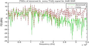
In the second stage, median filter is used. When the noise level is high, the noise is not suppressed completely by the SG filter. To reduce the noise further and to reduce the impulsive spikes, the signal x SG(n) is filtered using median filter. The output of median filter is the denoised signal, x (n). The parameters of the filter are selected in the same way as for SG filter. The threshold values selected are 0.7 and 0.75. With the filters in cascade, the noise is eliminated to a larger extent. The PSDs of the noisy signal, y (n) and the denoised signal x (n) are computed and plotted in Fig. 3. It may be observed that all the high-frequency components of the noise are attenuated, and the low-frequency components are smoothed. The same procedure is repeated with wavelet filter followed by median filter and it is found that the combination of SG filter with median filter is good.
PSDs of denoised and noisy waveforms of T 1 (n) code for −6 dB SNR.

Polyphase and polytime codes are analyzed and the parameters are estimated for various SNRs. The flow diagram for estimating the modulation parameters is shown in Fig. 2. The output of the median filter x(n) is analyzed using CS algorithm and the SCD coefficients $S_{x_N}^r$ (n, k) are computed.
Analysis of noise-free polyphase codes
Frank code is generated using equation (13). The sampling frequency f s is taken as 7 GHz for all the codes. Recall equation (27),

where x T(n) is the generated Frank code which is a noise-free signal. Since the analysis is for noise-free signals, w(n) = 0.
Therefore, y(n) = x T(n) = x(n) where x(n) is the denoised signal.
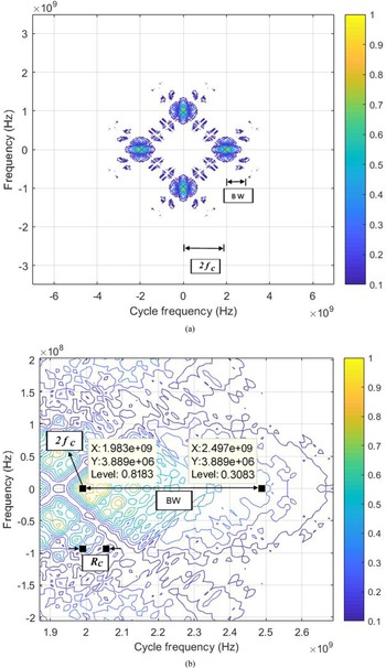
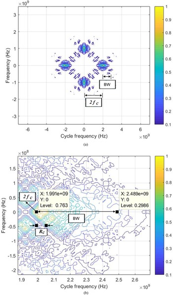
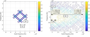
The SCD coefficients, $\;S_{x_N}^r ( {n, \;k} ) , \;$ of the noise-free Frank code, x(n) are calculated using equation (9). Figure 4 shows the bifrequency or the contour plot of $\;S_{x_N}^r ( {n, \;k} )$
 . Cycle frequency is represented on x-axis, frequency is represented on y-axis, and the color of the figure varies depending on $\;S_{x_N}^r ( {n, \;k} )$
 values. On careful observation, it is found that the plot is symmetric and spread in four patterns as shown in Fig. 4(a). The width from the center of the figure to the center of the right most pattern or the left most pattern along the x-axis gives 2f c. In other words, the x-coordinate of the center of the right most pattern is equal to 2f c and the color of the point is yellow. Figure 4(b) shows the close-up of the right most pattern of Fig. 4(a). From the figure, it can be written as, 2f c =1.983 GHz and hence f c = 0.9915 GHz. The difference between the center point and the end point of the selected pattern along the x-axis gives BW which is measured as 514 MHz (2.497e + 9−1.983e + 9 = 0.514e + 9). The code rate, R c is the difference between any two adjacent points along the x-axis which is measured as 8. Hence N c is calculated using the equation N c = BW/R c = 64.3. It may be mentioned that N c should satisfy the relation, N c = 2k, where k is any +ve integer. The nearest value of N c is 64. In the present case, N c = 64 is used. All the values are measured manually from Fig. 4(b) and the measured values are listed in the first row of Table 1. The error in estimation for all the parameters is calculated using equation (31).

Contour plot of noise-free Frank code for f c = 1 GHz. (a) Complete bi frequency plane, (b) close up of the selected segment for the measurement of BW and Rc.

Results obtained by the proposed and literature methods for Frank code

NA, not available.
Table 1 shows the comparison between the proposed method and values reported in the literature along with the percentage of estimation error. The second column shows the noise level of the modulated signal, the third column gives the measured parameter, and the fourth column gives the true values of the parameters. Columns 5 through 8 show the measured values, error in estimation using the proposed and the literature methods, respectively. The literature method [Reference Shyam sunder7] is discussed briefly in section “Denoising using MST (literature method)”.
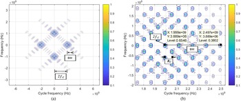
In the same way, P 1 code waveform is generated using equation (14) and the $S_{x_N}^r ( {n, \;k} )$ values are calculated using equation (9). The contour plot of $S_{x_N}^r ( {n, \;k} )$
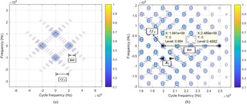
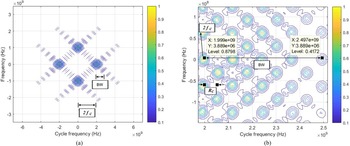
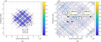
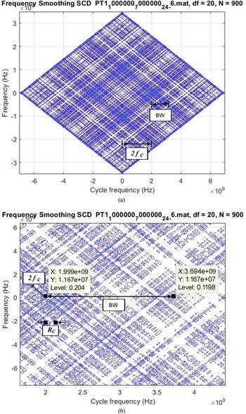
 is shown in Fig. 5. As explained for Frank code, the parameters f c, BW, and N c are measured as 999.5, 505, and 63.125, respectively, and the simulation results are shown in the first row of Table 2. The same procedure is repeated for P 2, P 3, and P 4 codes and the corresponding SCD coefficients are computed. The contour plots of P 2 through P 4 of noise-free waveforms are shown in Figs 6–8 and the measured values are noted in the first row of Tables 3–5, respectively.
Contour plot of noise-free P 1 code for f c = 1 GHz. (a) Complete bi frequency plane, (b) close up of the selected segment for the measurement of BW and Rc.

Contour plot of noise-free P 2 code for f c = 1 GHz. (a) Complete bi frequency plane, (b) close up of the selected segment for the measurement of BW and Rc.

Contour plot of noise-free P 3 code for f c = 1 GHz. (a) Complete bi frequency plane, (b) close up of the selected segment for the measurement of BW and Rc.

Contour plot of noise-free P 4 code for f c = 1 GHz. (a) Complete bi frequency plane, (b) close up of the selected segment for the measurement of BW and Rc.

Results obtained by the proposed and literature methods for P1 code

Results obtained by the proposed and literature methods for P2 code

Results obtained by the proposed and literature methods for P3 code

Results obtained by the proposed and literature methods for P4 code

Denoising using MST (literature method)
The MST coefficients of the noisy signal are computed first. The power content depends on the coefficient value. If the coefficient is high, then the power content is high and hence the coefficient belongs to the signal component. Since the power in the noise is less, the MST coefficient is also less. Select a suitable threshold value η p. All the MST coefficients greater than η p are called S-approximation coefficients and the remaining coefficients are called S-detailed coefficients. Similarly, a threshold value for noise η n is selected. The MST coefficients of the denoised signal are obtained by adding the S-approximation coefficients with the thresholded S-detailed coefficients. The denoised signal is obtained by computing the inverse MST.
Simulation results of polyphase codes under various noise conditions
Frank code is generated using equation (13). Here it is assumed that the signal received by the intercept receiver is corrupted with AWGN. Hence, white noise, w (n), is added to the generated Frank code as given in equation (27). The noisy signal, y(n) is denoised using SG filter and median filter as shown in Fig. 2. The SCD coefficients $, \;\;\;S_{x_N}^r ( {n, \;k} ) , \;\;$ are computed for the denoised signal, x (n). Figure 9 shows the contour plot of Frank code for −6 dB SNR. The parameters are measured from the figure as explained in section “Analysis of noise-free polyphase codes” and the values are noted in the second row of Table 1. In fact, the experiment is repeated for all noise levels up to −13 dB. But the results are tabulated for five sets of readings only. The third row shows the results for −7 dB SNR. The last two rows show the results for −12 and −13 dB.
Contour plot of noisy Frank code for f c = 1 GHz (−6 dB SNR). (a) Complete bi frequency plane for −6 dB, (b) close up of the selected segment for the measurement of BW and Rc for −6 dB.

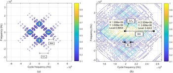
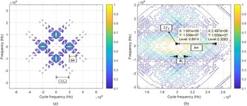
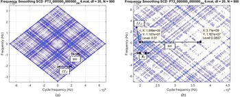
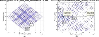
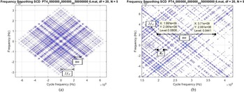
For the other polyphase codes also, the SCD coefficients, $\;S_{x_N}^r ( {n, \;k} )$ are calculated under various noise conditions. Figures 10–13 show the contour plots of P 1, P 2, P 3, and P 4 codes, respectively, for −6 dB SNR. The parameters are estimated as explained in section “Analysis of noise-free polyphase codes” and the corresponding values are shown in the second row of Tables 2–5 respectively. With the proposed method, it is clear from the tables that the accuracy of measurement is >95% for all codes up to −12 dB SNR. But when the noise is high (SNR < −12 dB), the error in estimation is more than 5% and the process is stopped at −13 dB SNR. The values reported in the literature for the polyphase codes are available up to −7 dB SNR only as the error in estimation is more than 5% for low SNRs [Reference Shyam sunder7]. From the tables and Figs 4–14, it is clear that the proposed method is better compared to the literature method. The same procedure is extended to the analysis of noisy polytime codes.
Contour plot of noisy P 1 code for f c = 1 GHz (−6 dB SNR). (a) Complete bi frequency plane for-6dB, (b) close up of the selected segment for the measurement of BW and Rc for −6 dB.

Contour plot of noisy P 2 code for f c = 1 GHz (−6 dB SNR). (a) Complete bi frequency plane for −6 dB, (b) close up of the selected segment for the measurement of BW and Rc for −6 dB.

Contour plot of noisy P 3 code for f c = 1 GHz (−6 dB SNR). (a) Complete bi frequency plane for −6 dB, (b) close up of the selected segment for the measurement of BW and Rc for −6 dB.

Contour plot of noisy P 4 code for f c = 1 GHz (−6 dB SNR). (a) Complete bi frequency plane for −6 dB, (b) close up of the selected segment for the measurement of BW and Rc for −6 dB.

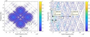
Contour plot of T 1 code for f c = 1 GHz for −6 dB SNR. (a) Complete bi frequency plane, (b) closer approximation of the selected segment for the measurement of BW and Rc.

Analysis of polytime codes (T 1−T 4) under various noise conditions
Analysis of noise-free polytime codes (T 1−T 4) using CS method is reported in [Reference Chilukuri, Kakarla and Subbarao6, Reference Shyam Sunder and Subbarao12]. It was assumed that the received signals were free from noise. All the parameters were estimated with an accuracy of better than 95%. Since the signals are generally corrupted with noise, the analysis of noisy signals is considered here. In this case also, the noisy signals are denoised using SG and median filters and then CS techniques are used for the estimation of the parameters.
T 1(n) code is generated using equation (18) and white noise is added to the signal as given in equation (27). The noisy signal is denoised as explained in section “Denoising techniques” and the SCD coefficients $\;S_{x_N}^r ( {n, \;k} )$ are calculated. Figure 14 shows the contour plot of T 1(n) code for SNR = −6 dB. The parameters f c, BW, and R c are estimated as shown in the figure. The first row of Table 6 shows the measured values and the error in estimation for SNR = −6 dB. The error in the measured values is <5% for all the parameters. It may be mentioned here that estimated values are not available in the literature for denoised polytime codes. The analysis is carried out for all noise levels up to −13 dB SNR. But the results are shown in the table for −6, −12, and −13 dB only. The other polytime codes are also analyzed using the same procedure. Figures 15–17 show the SCD patterns for T 2(n), T 3(n), and T 4(n), respectively, and the measured values are shown in Tables 7–9 for various SNRs. For polytime codes also, the error in estimation is <5% for SNRs up to −12 dB. With the proposed method, we are able to extract the parameters of both polyphase and polytime codes with an accuracy of better than 95% up to −12 dB SNR which is a significant improvement compared to the literature values.
Contour plot of T 2 code for f c = 1 GHz for −6 dB SNR. (a) Complete bi frequency plane, (b) closer approximation of the selected segment for the measurement of BW and Rc.

Contour plot of T 3 code for f c = 1 GHz for −6 dB SNR. (a) Complete bi frequency plane, (b) closer approximation of the selected segment for the measurement of BW and Rc.

Contour plot of T 4 code for f c = 1 GHz for −6 dB SNR. (a) Complete bi frequency plane, (b) closer approximation of the selected segment for the measurement of BW and Rc.

Results obtained for T1 code for various SNRs

Results obtained for T 2 code for various SNRs

Results obtained for T3 code for various SNRs

Results obtained for T4 code for various SNRs

Conclusions
LPI radar waveforms are analyzed using CS algorithm to estimate the modulation parameters such as carrier frequency, band width, and number of subcodes. Precise measurement of intrapulse parameters and the knowledge of the type of the waveform will give the information about the threat to the radar so that the EA or ES system could take instantaneous counter action against the enemy. Generally, the signals received by the intercept receiver are corrupted with noise. To improve the signal quality and the measurement accuracy, the noisy signal is pre-processed using two types of denoising filters namely SG filter and median filter. The denoised signal is analyzed using CS techniques. The CS algorithm is the most suitable algorithm for the analysis of periodic signals such as LPI radar waveforms. With the proposed method, we are able to extract the parameters of both polyphase and polytime codes with an accuracy of better than 95% up to the noise level of −12 dB SNR. The estimation error is more than 10% when the noise level is very high (<−12 dB). The parameters extracted are bandwidth, carrier frequency, and code rate. On comparison with the literature values, it is found that the present method is superior. The main advantage of the present work is that the same algorithm gives good results for both polyphase and polytime codes upto −12 dB SNR.
Acknowledgements
The authors express their sincere thanks to the management and principal, VNRVJIET, Hyderabad for providing necessary facilities to carry out this work.
 Chilukuri Raja Kumari was born in Krishna District, Andhra Pradesh, India. She received the B.E. degree (ECE) from Anna University, the M.Tech. degree from Dr. M.G.R University, Tamil Nadu, India. She is pursuing her Ph.D. degree in the field of VLSI signal processing from Koneru Lakshmaiah University (KLEF), Vijayawada, Andhra Pradesh, India. She received university first rank in PG Study. She is also a recipient of gold medal. Presently she is working as an Assistant Professor in the Department of Electronics and Communication Engineering, VNRVJIET. She has published five international journals and three conferences. She is a Reviewer for few national journals. Her research interests include VLSI and radar signal processing. She is a life member of ISTE, IEI, and IAENG. She is also a member of IEEE.
 Dr. Hari Kishore Kakarla was born in Vijayawada, Andhra Pradesh, India. He received the B.Tech. degree (ECE) from JNTUH, the M.Tech. degree from SK University, AP, India. He received his Ph.D. degree in the field of VLSI from Koneru Lakshmaiah University (KLEF). He received his Postdoctoral Fellowship (PDF) in Malaysia. He is working as a Professor in Electronics and Communication Engineering. He has published three IEEE Transactions and more than 124 research articles in international journals/conferences with H-index of 32. He has filled seven patents and published three textbooks. He is an Editorial Board Member/Reviewer for several international journals/conferences. His research interests include VLSI, fault tolerance and digital testing, IOT, communications and signal processing. He is a life member of ISTE, IE, IACSIT, and IAENG.
 Prof. K. Subba Rao worked in Osmania University (OU) for 31 years in various capacities. He was superannuated from OU in October 2011. He has published 150 research papers in international and national journals/conferences. Under his supervision, nine candidates were awarded Ph.D. degrees. He visited countries such as Saudi Arabia, USA, and Japan and participated in conferences. Under SONET program, he has delivered more than 25 lectures on the subject “Digital Signal Processing” as per the JNTU syllabus. He has conducted several short-term courses in OU and various organizations such as DRDO and ECIL. He has successfully completed four major research projects sponsored by AICTE, DRDO, and Analog Devices, Bangalore in the areas of radar and multimedia signal processing. He has successfully completed two CARS projects sponsored by RCI, DRDO, Hyderabad. His areas of research interests include signal processing, signal design and modelling of biological systems.