2 Analysis: shallow water theory

2.1 Vertical averaging across the liquid height

In the present study, shallow water equations with vertical averaging of the flow field are used to predict the free surface profiles upstream and downstream of a steady hydraulic jump for slight inclinations from the horizontal orientation. In addition, a force balance across the jump is used to locate the jump position (Kasimov Reference Kasimov2008; Bonn et al. Reference Bonn, Andersen and Bohr2009). Surface tension is neglected as it does not govern the flow structure (Bohr et al. Reference Bohr, Putkaradze and Watanabe1997) although it decides flow stability (not discussed in this paper). Based on the common assumptions of shallow water theory, the local continuity equation for an incompressible fluid in the planar geometry is

(2.1)$$\begin{eqnarray}\frac{\unicode[STIX]{x2202}u}{\unicode[STIX]{x2202}x}+\frac{\unicode[STIX]{x2202}w}{\unicode[STIX]{x2202}z}=0,\end{eqnarray}$$

and the pertinent momentum equation (similar to the boundary-layer flow equation) is

(2.2)$$\begin{eqnarray}u\frac{\unicode[STIX]{x2202}u}{\unicode[STIX]{x2202}x}+w\frac{\unicode[STIX]{x2202}u}{\unicode[STIX]{x2202}z}=-g\cos \unicode[STIX]{x1D703}\frac{\text{d}h}{\text{d}x}+\unicode[STIX]{x1D708}_{l}\frac{\unicode[STIX]{x2202}^{2}u}{\unicode[STIX]{x2202}z^{2}}\pm g\sin \unicode[STIX]{x1D703}.\end{eqnarray}$$

The nomenclatures used in (2.1) and (2.2) are explained in figure 1; $+$ve sign precedes $g\sin \unicode[STIX]{x1D703}$ for downslope flows and a $-$ve sign denotes adverse slope, where $\unicode[STIX]{x1D703}$ gives the absolute value of angle of inclination.

Further, the condition for constant volume flux gives

(2.3)$$\begin{eqnarray}q=\frac{Q}{W}=\int _{0}^{h}u(x,z)\,\text{d}z,\end{eqnarray}$$

where $q$ is the volumetric flow rate per unit channel width. The boundary conditions are no slip and no penetration on the bottom wall and zero shear stress at the free surface (for stagnant air above the free surface)

(2.4a,b)$$\begin{eqnarray}u(x,0)=w(x,0)=0,\quad \left.\frac{\unicode[STIX]{x2202}u}{\unicode[STIX]{x2202}z}\right|_{z=h(x)}=0.\end{eqnarray}$$

The scaling parameters obtained from the order of magnitude analysis of (2.1)–(2.3), viz. $u^{C}=q^{1/3}g^{1/3}\cos \unicode[STIX]{x1D703}^{1/3}$, $w^{C}=q^{-2/3}\unicode[STIX]{x1D708}_{l}g^{1/3}\cos \unicode[STIX]{x1D703}^{1/3}$, $x^{C}=q^{5/3}{\unicode[STIX]{x1D708}_{l}}^{-1}g^{-1/3}\cos \unicode[STIX]{x1D703}^{-1/3}$ and $z^{C}={q_{l}}^{2/3}g^{-1/3}\cos \unicode[STIX]{x1D703}^{-1/3}$, yield the rescaled equations

(2.5)$$\begin{eqnarray}\displaystyle & \displaystyle \frac{\unicode[STIX]{x2202}u}{\unicode[STIX]{x2202}x}+\frac{\unicode[STIX]{x2202}w}{\unicode[STIX]{x2202}z}=0, & \displaystyle\end{eqnarray}$$

(2.6)$$\begin{eqnarray}\displaystyle & \displaystyle u\frac{\unicode[STIX]{x2202}u}{\unicode[STIX]{x2202}x}+w\frac{\unicode[STIX]{x2202}u}{\unicode[STIX]{x2202}z}=-\frac{\text{d}h}{\text{d}x}+\frac{\unicode[STIX]{x2202}^{2}u}{\unicode[STIX]{x2202}z^{2}}\pm A, & \displaystyle\end{eqnarray}$$

(2.7)$$\begin{eqnarray}\displaystyle & \displaystyle \int _{0}^{h(x)}u(x,z)\,\text{d}z=1, & \displaystyle\end{eqnarray}$$

where $A=q{\unicode[STIX]{x1D708}_{l}}^{-1}\tan \unicode[STIX]{x1D703}$. The corresponding boundary conditions are

(2.8a-c)$$\begin{eqnarray}u(x,0)=0,\quad w(x,0)=0,\quad \left.\frac{\unicode[STIX]{x2202}u}{\unicode[STIX]{x2202}z}\right|_{z=h(x)}=0.\end{eqnarray}$$

Integrating (2.5) and (2.6) from $z=0$ to $z=h(x)$ and incorporating boundary conditions, the following averaged momentum equation is obtained

(2.9)$$\begin{eqnarray}V_{av}\frac{\text{d}}{\text{d}x}(FV_{av})=-\frac{\text{d}h}{\text{d}x}-\frac{1}{h}\left.\frac{\unicode[STIX]{x2202}u}{\unicode[STIX]{x2202}z}\right|_{z=0}\pm A,\end{eqnarray}$$

where the average velocity $V_{av}$ is defined as $V_{av}=(1/h)\int _{0}^{h}u(x,z)\,\text{d}z$ and $F=(\int _{0}^{h}u^{2}\,\text{d}z)/(hV_{av}^{2})$. The mass conservation condition (2.7) yields $V_{av}h=1$.

Based on the numerical results (§ 4) which display self-similar parabolic velocity profiles upstream and downstream of the jump, we consider

(2.10)$$\begin{eqnarray}u(x,z)=V_{av}(x)f(\unicode[STIX]{x1D702}),\end{eqnarray}$$

where $\unicode[STIX]{x1D702}=z/h(x)$ and $0\leqslant \unicode[STIX]{x1D702}\leqslant 1$. Equation (2.10) must satisfy the mass flux and boundary conditions, which implies $f(0)=0$, $f^{\prime }(1)=0$ and $\int _{0}^{1}f(\unicode[STIX]{x1D702})\,\text{d}\unicode[STIX]{x1D702}=1$. Based on this, a simple and physically reasonable parabolic profile has been considered for laminar flow in a thin film

(2.11)$$\begin{eqnarray}f(\unicode[STIX]{x1D702})=3\unicode[STIX]{x1D702}-{\textstyle \frac{3}{2}}\unicode[STIX]{x1D702}^{2}.\end{eqnarray}$$

This gives $F={\textstyle \frac{6}{5}}=K_{1}$ and $\unicode[STIX]{x2202}u/\unicode[STIX]{x2202}z|_{z=0}=3V_{av}/h=K_{2}V_{av}/h$. Constants $K_{1}$ and $K_{2}$ depend on the velocity profile only.

Equation (2.9) is now reduced to

(2.12)$$\begin{eqnarray}K_{1}V_{av}\frac{\text{d}V_{av}}{\text{d}x}=-\frac{\text{d}h}{\text{d}x}-\frac{K_{2}V_{av}}{h^{2}}\pm A.\end{eqnarray}$$

The scales obtained from the order of magnitude analysis of (2.12), $V_{av}^{R}=K_{1}^{-1/3}$,$h^{R}=K_{1}^{1/3}$ and $x^{R}=K_{1}^{4/3}K_{2}^{-1}$ transform (2.12) to a general form as

(2.13)$$\begin{eqnarray}V_{av}\frac{\text{d}V_{av}}{\text{d}x}=-\frac{\text{d}h}{\text{d}x}-\frac{V_{av}}{h^{2}}\pm B,\end{eqnarray}$$

where $B=K_{1}K_{2}^{-1}A$. It may be noted that, although the values of $K_{1}$ and $K_{2}$ may change depending upon the velocity distribution across the liquid height, the general form of the above equation remains the same.

Incorporation of the mass conservation condition in (2.13) leads to

(2.14)$$\begin{eqnarray}\frac{\text{d}h}{\text{d}x}=\frac{1\mp Bh^{3}}{1-h^{3}},\end{eqnarray}$$

where the $-$ve sign before $B$ is applicable to downward inclinations, the $+$ve sign is used for upslope flows and $B=0$ for horizontal flow.

2.2 Connecting upstream and downstream solutions

The solutions upstream and downstream of the jump can be linked by means of a Rayleigh’s shock (Rayleigh Reference Rayleigh1914) across which mass and momentum flux are conserved. Assuming friction within the jump region to be negligible, the momentum equation for jumps in inclined channels can be written as

(2.15)$$\begin{eqnarray}\frac{1}{2}\unicode[STIX]{x1D70C}_{l}gh_{1}^{2}\cos \unicode[STIX]{x1D703}-\frac{1}{2}\unicode[STIX]{x1D70C}_{l}gh_{2}^{2}\cos \unicode[STIX]{x1D703}\pm \frac{1}{2}S\unicode[STIX]{x1D70C}_{l}gL(h_{1}+h_{2})\sin \unicode[STIX]{x1D703}=\unicode[STIX]{x1D70C}_{l}\int _{0}^{h_{2}}u_{2}^{2}(z)\,\text{d}z-\unicode[STIX]{x1D70C}_{l}\int _{0}^{h_{1}}u_{1}^{2}(z)\,\text{d}z,\end{eqnarray}$$

where subscripts 1 and 2 correspond to positions immediately upstream and downstream of the jump, $L$ is the distance between 1 and 2 and $S$ is a shape factor which takes care of the actual surface profile in the jump region. The third term on left-hand side of (2.15) accounts for the weight component of the fluid contained in the jump region and is thus $+$ve for downslope, $-$ve for adverse slopes and zero for horizontal flow.

Using the depth averaged velocity and mass conservation condition, equation (2.15) can be rewritten as

(2.16)$$\begin{eqnarray}\frac{1}{2}g(h_{1}^{2}-h_{2}^{2})\cos \unicode[STIX]{x1D703}\pm \frac{1}{2}SgL(h_{1}+h_{2})\sin \unicode[STIX]{x1D703}=F\frac{q^{2}}{h_{2}}-F\frac{q^{2}}{h_{1}},\end{eqnarray}$$

based on similar velocity profiles upstream and downstream of the jump, for which $F_{1}=F_{2}=F$. The non-trivial solution obtained from the above cubic equation is as follows:

(2.17)$$\begin{eqnarray}h_{2}=\frac{h_{1}}{2}\left(\sqrt{1+\frac{8FFr_{1}^{2}}{\cos \unicode[STIX]{x1D703}\mp {\displaystyle \frac{SL}{h_{2}-h_{1}}}\sin \unicode[STIX]{x1D703}}}-1\right),\end{eqnarray}$$

where $Fr_{1}(=V_{1}/\sqrt{gh_{1}})$ is the Froude number immediately upstream of the jump.

Most of the previous studies on downslope flows have assumed $S=(h_{2}-h_{1})/L$. Although the assumption has no strong fundamental basis, we obtain model predictions close to experimental results (as shall be seen in § 6). So the same has been adopted in the present analysis to obtain the jump strength from (2.17)

(2.18)$$\begin{eqnarray}\frac{h_{2}}{h_{1}}=\frac{\sqrt{1+8FFr_{m,1}^{2}}-1}{2},\end{eqnarray}$$

where the Froude number (the natural dimensionless number for this phenomenon) has been obtained from mass and momentum balance across the jump.

(2.19)$$\begin{eqnarray}Fr_{m}=\frac{Fr}{\sqrt{\cos \unicode[STIX]{x1D703}\mp \sin \unicode[STIX]{x1D703}}}.\end{eqnarray}$$

We note that (2.18) reduces to the Bélanger equation (classical jump equation based on inviscid theory) for $F=1$ and $Fr_{m,1}=Fr_{1}$. It is important to note that, in (2.19), the Froude number incorporates the effect of inclination through the term $\cos \unicode[STIX]{x1D703}\mp \sin \unicode[STIX]{x1D703}$ ($-$ve and $+$ve signs pertaining to downslope and upslope flows respectively and for horizontal flow $Fr_{m}$ reduces to $Fr$). This is different from the straightforward inclusion of a gravity component to describe buoyancy forces in single phase flow and suggests that a laminar hydraulic jump cannot be regarded as a simple problem of single phase flow over sloped channels.

Figure 2.

Typical solution of shallow water theory. The blue solid curves represent the upstream and the downstream solutions from (2.14), and the dashed magenta curve shows the height to which upstream flow is expected to rise based on the jump condition (2.18). The intersection of downstream heights obtained from (2.14) and (2.18) represents the jump location (blue dotted line).

2.3 Solution methodology

We solve (2.14) numerically by using the standard Runge–Kutta method of fourth order and obtain the supercritical flow solution upstream of the jump (curve AB in figure 2) from the inlet boundary condition ($h=h_{in}$ at $x=0$). The subcritical flow solution downstream of the jump (curve CD in figure 2) is obtained by using an outlet boundary condition. This is a critical parameter in the analysis and it is difficult to precisely define this condition since, at the outlet, liquid runs off the channel with an appreciable curvature of the streamline. A survey of the past literature suggests that several researchers (Higuera Reference Higuera1994; Singha et al. Reference Singha, Bhattacharjee and Ray2005; Bonn et al. Reference Bonn, Andersen and Bohr2009) have assumed the exit liquid height to be critical. The same can be shown by energy balance and has also been obtained from our numerical results, discussed later. Accordingly, we consider the liquid height to be critical ($h=1$) at the end of the channel. Since the solution is singular at $h=1$, we start the solution slightly before the channel end, where the liquid height is slightly above the critical value. Figure 2 presents the typical solutions upstream and downstream of the jump for all channel inclinations. The solution predicts $h$ to increase with $x$ in the upstream section and decrease downstream as one moves away from the jump. At $h=1$ the upstream solution diverges, which is a characteristic of shallow water theory well documented in the literature (Bohr et al. Reference Bohr, Dimon and Putkaradze1993; Singha et al. Reference Singha, Bhattacharjee and Ray2005). To overcome this limitation, we use the jump condition (2.18) to pinpoint the jump location ($x_{j}$) as the point of intersection of downstream heights obtained from (2.14) and (2.18).

Figure 3.

Evolution of the free surface profile in normalized time $t/(h_{in}/u_{in})$ for $Re=87.5$ and $L_{c}/h_{in}=360$. The free surface profiles are depicted for different time instants ($t$) scaled with the time required for the liquid layer to travel its inlet height ($h_{in}$) at inlet velocity ($u_{in}$).

3 Numerical simulation

Although the shallow water theory has successfully predicted jump parameters in inclined channels, it exhibits a discontinuity at the jump. Therefore, to understand the physics in the vicinity of the jump, extensive numerical simulations have been performed using the open source code, Gerris, following the methodology of Dasgupta et al. (Reference Dasgupta, Tomar and Govindarajan2015). They have simulated jumps for horizontal channels and we have used the same for numerical simulation in inclined channels (figure 1) for both upslope and downslope flows. The phenomenon is modelled as a two phase flow problem with stagnant air above the liquid region. Usual no-slip and no-penetration boundary conditions are imposed for the solid wall and the classical outflow boundary condition (i.e. Dirichlet in pressure and Neumann in velocity) is employed at the outlet boundary $O$ (figure 1). As shown in figure 1, the end of the channel is attached to a straight wall projected downward to ensure smooth liquid drainage from the computational domain.

Gerris solves the transient incompressible Navier–Stokes equation, following a finite volume approach and uses a second-order accurate staggered-in-time discretization over the entire domain for volume fraction, density, velocity and pressure fields. For spatial discretization in the entire domain, Gerris uses a quad/oct tree mesh refinement technique (Popinet Reference Popinet2003). In the present case, efficient mesh refinement and adaptation are based on predefined criteria for vorticity and the gradient of the liquid fraction. The predefined maximum refinement takes place only at the required locations and time depending on the defined criteria. Examining the simulations with higher and lower refinement levels, the grid independent refinement level has been adopted. The details for the understanding and implementation of Gerris are provided in Popinet (Reference Popinet2003, Reference Popinet2009) and Dasgupta et al. (Reference Dasgupta, Tomar and Govindarajan2015).

4 Simulation results

For a comprehensive understanding of the hydrodynamics of flow, the results have been presented for different Reynolds numbers in figures 3–7. Initially, the transient evolution of the free surface profile is discussed for a representative flow situation in figure 3 and then the steady state results are presented at four different channel positions, namely before and after the jump, at the jump and near the channel exit in figure 4 to illustrate the axial development of the flow. The corresponding development of the pressure profile is presented in figure 5. The results for two higher Reynolds numbers are presented in figures 6 and 7. Streamline patterns have been included in figures 4, 6 and 7 to identify the jump type and vorticity (indicated by a closed streamline). In order to extend the results to similar flows occurring at different scales, the parameters are depicted in dimensionless terms ($u$ scaled with maximum axial velocity, $U_{max}$, at that location, $z$ with local height $h$ of the free surface and $x$ with the inlet liquid height $h_{in}$).

Figure 4.

Planar hydraulic jump for $Re=87.5$ and $L_{c}/h_{in}=360$. (a) Streamline patterns and the free surface profile. Axial velocity distribution, scaled with maximum axial velocity at that particular location for (b) upstream of the jump, (c) jump region, (d) downstream of the jump and (e) exit from the channel.

Figure 5.

Pressure distribution on the channel floor for $Re=87.5$ and $L_{c}/h_{in}=360$. Red dashed-dot curve and blue continuous curve represent the fluid pressure and the hydrostatic component of the fluid pressure respectively. The hydrostatic pressure is evaluated from the weight of the liquid column ($\unicode[STIX]{x1D70C}_{l}gh$) above the bottom wall.

Figure 6.

Planar hydraulic jump for $Re=137.5$ and $L_{c}/h_{in}=360$. (a) Streamline patterns and the free surface profile. Axial velocity distribution, scaled with maximum axial velocity at the same location for (b) upstream of the jump, (c) jump region and (d) downstream of the jump.

Figure 7.

No jump is formed for $Re=175$ and $L_{c}/h_{in}=360$. Streamline patterns and the free surface profile.

The transient evolution of the free surface profile is presented in figure 3 for the Reynolds number $Re=q/\unicode[STIX]{x1D708}_{l}=87.5$ and $L_{c}/h_{in}=360$. The figure shows that the simulation results attain steady state after a reasonable period of time. During this period, the liquid layer of local height $h$ proceeds towards the channel exit and a jump-like structure forms due to viscous dissipation. Once the liquid layer reaches the channel exit, the liquid falls freely from the channel floor and the boundary condition at the exit changes. The height of the liquid film at the exit end gradually increases and the information of the increased height propagates upstream (blue curves in figure 3). As expected, this upstream propagation of information is confined within the subcritical region of the flow (i.e. the region downstream of the jump). Consequently, the overall height of the post-jump liquid layer increases while the free surface upstream of the jump remains unchanged. The flow structure eventually stabilizes and the jump becomes stationary at a certain location.

Figure 4 depicts the streamline patterns and free surface profile, along with the axial evolution of the velocity profile after the flow attains the steady state. We observe that the flow upstream of the jump decelerates and, as a consequence, the height of the free surface increases while in the downstream region the slope of the free surface is negative, the trends being similar to the shallow water results. Just after the inlet section, the axial velocity distribution across the liquid height follows a parabolic profile and evolves along the axial direction for a short distance. Beyond the flow development zone (close to the inlet), the shape of the velocity profile does not evolve any further up to the jump region, retaining its parabolic shape with the maximum streamwise velocity on the free surface. The profiles exhibit self-similarity both upstream and downstream of the jump, thus justifying (2.10) in shallow water theory. Nevertheless, in the jump region (figure 4c), the self-similarity is completely destroyed. This is because the liquid height abruptly increases and the free surface profile becomes very steep. In addition, undulations appear at the free surface depending on the flow conditions and the maximum axial velocity may not always occur at the free surface. The velocity profiles (in figure 4c) further display flow separation near the floor, indicating local flow reversal. This phenomenon is similar to boundary-layer separation for flow over a solid surface and suggests the predominance of form friction during the transition from super- to subcritical flow. Nevertheless, the physics of the flow is different in the two cases. While boundary-layer separation is caused by the adverse pressure gradient imposed by inviscid flow external to the boundary layer, the thin film in the present case flows with a free surface where external inviscid flow is absent but the hydrostatic pressure gradient is dominant due to the abrupt elevation of the free surface. This is evident from the pressure distribution along the channel floor. Figure 5 shows that the fluid pressure is almost close to the hydrostatic pressure everywhere, except near the jump. This adverse pressure gradient along the floor causes flow separation and vortex formation at the jump, as displayed by the closed streamline patterns near the floor in figure 4(a).

Near the channel exit, the velocity profile again changes (figure 4e) as the flow is accelerated by gravity while it takes an almost $90^{\circ }$ turn and the maximum streamwise velocity occurs close to the channel floor, far below the free surface.

The results for higher $Re$ presented in figures 6 and 7 show that an increase in Reynolds number results in a weaker jump (lower elevation of the free surface) shifted towards the exit. At still higher $Re$ (figure 7) there is no jump and the flow remains supercritical throughout the channel length. This is an expected outcome since the increased inertial force overcomes the viscous forces necessary for the required flow deceleration to a subcritical condition. Figure 6 also shows that, for a higher $Re$, the hydrostatically generated adverse pressure gradient is not strong enough to cause flow separation and vortex formation. From a close comparison of figures 4 and 6, we further note that $Re$ primarily influences the jump structure and location, while the other features, such as the nature of velocity distribution and free surface profile upstream and downstream of the jump, remain the same. In all cases, the velocity profiles are self-similar both before and after the jump (except close to the inlet and exit) and at the exit, profiles similar to that depicted in figure 4(e) (not shown for conciseness) are obtained. Interestingly, the upstream free surface profiles follow the expression $\text{d}h/\text{d}x=1.81/Re$ proposed by Watson (Reference Watson1964). This is contrary to the results reported by Bonn et al. (Reference Bonn, Andersen and Bohr2009) for narrow channels with a width of the order of the liquid height. Their observation that the upstream free surface profile is independent of $Re$ can be attributed to the enhancement of the viscous effect from the closely spaced side walls. In our case, since the channel width is sufficiently large compared to the maximum liquid height (occurring downstream of the jump), the associated side wall effects are negligible and, due to the interplay of inertial and viscous forces, the slope of the free surface upstream of the jump is not independent of $Re$.

Figure 8.

Schematic of the experimental facility. The electrical conductivity principle is used to measure the free surface depth. The measurement system consists of a point electrode connected to the digital depth micrometer (DD). To examine the continuity, a digital multimeter (MM) is used. The external circuit is made using electrical connecting wires W1 and W2. W1 connects the depth micrometer with one terminal of the multimeter, while W2 makes the connection between the other terminal and water.

5 Experimental investigation

In order to validate the results of the numerical simulations and the predictions from shallow water theory, experiments have been designed to generate thin film flow in a rectangular channel 10 cm wide with side walls of 2 cm height. The selected channel width minimizes side wall effects to approach the approximation of two-dimensional flow. Three different channel lengths of 3, 6 and 9 cm have been selected to investigate the effect of channel length on jump type (as shall be seen in figure 18). The channel dimensions are selected to ensure that the hydraulic jump is contained within the channel over the entire range of experimental parameters and the height of the liquid layer can be regarded as ‘thin’ (laminar flow condition) both before and after the jump. The channel is mounted on levelling screws in order to tilt it and align it perfectly at the desired inclination. The angle of inclination with horizontal is measured by a digital protractor with a resolution of $0.05^{\circ }$.

As depicted in figure 8, the set-up comprises of a closed-loop flow system where water from the main reservoir is circulated by a centrifugal pump to a constant-head tank via a Coriolis mass flow meter and after flowing through the channel, water discharges into the collecting tank (CT). To obtain the volumetric flow rate at the entry, the volumetric flow of liquid to the collecting tank is measured and a calibration curve is generated to estimate the liquid flow rate as a function of liquid height in the constant-head tank (CH). The constant water level at the tank is varied with the help of a bypass valve (BV) to obtain the desired flow velocity.

Since boundary conditions are key parameters in thin film experiments through small dimension channels, special care has been taken to design the entry and exit sections. At the entry, the depth of the liquid film is controlled by a sluice gate (G) which forms the right wall of a constant-head tank and a flow distributor (FD) ensures a uniform velocity through the gate opening. The gate opening is kept constant at 0.25 mm in order to maintain a constant value of $h_{in}$ in all the experiments. The small uniform gap between the gate and the floor of the tank forces water to flow as a thin film of uniform thickness across the width. The edge of the gate is straight and sharp to ensure an opening normal to the channel axis and to minimize the resistance at the liquid inlet. Special care has been taken to secure a leak proof operation.

The importance of the exit condition on fluid draining and the jump parameters has been widely acknowledged for both circular and planar jumps. The sensitivity of the jump parameters to the exit conditions has been discussed at length by Duchesne, Lebon & Limat (Reference Duchesne, Lebon and Limat2014) for circular hydraulic jumps. Researchers determining the solution of the shallow water equations for circular jumps have also specified exit conditions and numerical studies (Dasgupta et al. Reference Dasgupta, Tomar and Govindarajan2015; Dasgupta & Tomar Reference Dasgupta and Tomar2015) have included the liquid exit in their computational domain. In the present study, experiments are performed to validate the results of theory and simulation, and thus the exit is designed to mimic the exit region of the computational domain (figure 1). Accordingly, a downward projected face is attached to the channel end perfectly at $90^{\circ }$ to guide the free fall of water. The corners at the exit are provided with a chamfering of 0.5 mm radius to ensure a smooth streamline curvature during vertical acceleration of the fluid.

Figure 9.

Photographic view of a typical hydraulic jump in thin film flow through a wide channel.

Since the downstream drainage effect (the small chamfering) is decisive for channels of relatively smaller dimensions, especially with regard to location, strength, stability and also the type of jump, we have performed a few experiments with different extents (radii) of the corner chamfering. Our observations reveal that liquid can drain with greater ease along smoothened corners. As the chamfering radius increases, the jump position shifts downstream and the strength decreases, thus favouring the transition from wavy to smooth and then to no jump condition. This suggests the need for a detailed study on the effect of downstream drainage on planar jump characteristics. However, in the present paper, the primary focus is on understanding the influence of the flow velocity and channel inclination on the jump characteristics. So we have performed all the reported experiments with the same exit conditions, i.e. with a chamfering radius of 0.5 mm. A similar chamfered exit was adopted by Kate et al. (Reference Kate, Das and Chakraborty2007a), Kate, Das & Chakraborty (Reference Kate, Das and Chakraborty2007b, Reference Kate, Das and Chakraborty2008) in their experiments on circular hydraulic jumps.

Figure 10.

Free surface profiles for $q=7.5\times 10^{-5}~\text{m}^{2}~\text{s}^{-1}$, $L_{c}=90~\text{mm}$ and $\unicode[STIX]{x1D703}=$ (a) $0^{\circ }$, (b) $0.3^{\circ }$ and (c) $0.6^{\circ }$. Points (diamond symbols) represent experimental data; red solid curve A represents the numerical solution and blue solid curve B represents the analytical solution. The magenta dashed curve shows the height to which upstream flow is expected to jump based on the jump condition. Analytically obtained jump location is shown by the blue dotted line.

Figure 11.

Free surface profiles for $q=12.5\times 10^{-5}~\text{m}^{2}~\text{s}^{-1}$, $L_{c}=90~\text{mm}$ and $\unicode[STIX]{x1D703}=$ (a) $0^{\circ }$, (b) $-0.3^{\circ }$ and (c) $-0.6^{\circ }$. Points (diamond symbols) represent experimental data; red solid curve A represents numerical solution and blue solid curve B represents analytical solution. The magenta dashed curve shows the height to which upstream flow is expected to jump based on the jump condition. Analytically obtained jump location is shown by the blue dotted line.

The free surface profile along the channel length is estimated by measuring the depth of the water layer at different axial locations by a digital depth micrometer (DD; lowest count of 0.01 mm and accuracy of $\pm 0.02~\text{mm}$). It employs a conductivity (electrical) principle to identify the gas–liquid interface. The same has been adopted by a number of researchers (Arakeri & Rao Reference Arakeri and Rao1996; Kate et al. Reference Kate, Das and Chakraborty2008; Vishwanath et al. Reference Vishwanath, Dasgupta, Govindarajan and Sreenivas2016) to measure film thickness in viscous hydraulic jumps. Each experiment is repeated at least three times to verify the reproducibility of the results. The error bars in the experimental data depict the spread obtained by repeating the experiments for the same flow conditions.

The experimental data are reported for $-0.6^{\circ }\leqslant \unicode[STIX]{x1D703}\leqslant 1.5^{\circ }$ and $5\times 10^{-5}\leqslant q\leqslant 19\times 10^{-5}~\text{m}^{2}~\text{s}^{-1}$. Figure 9 displays a snapshot of thin film planar jump observed in the present experiments. From experimental measurements, it is observed that the height of the free surface upstream of the jump increases linearly (as is evident from figures 10 and 11) while after the jump, the profile exhibits a decreasing trend and finally displays a sharp drooping nature at the channel exit where liquid falls off freely. The large standard deviation (error bars in figures 10 and 11) of the data points in the jump region also denotes a large fluctuation of the free surface across the jump. From flow visualization and measurements of the free surface height, we distinguish a variety of jumps namely – (i) submerged jump (Chow Reference Chow1959) where the flow occurs with an elevated free surface right from the entry and exhibits a descending profile all along the channel length, (ii) wavy jump with significant undulations of the free surface in the jump region, (iii) smooth jump, where the increase in free surface height occurs smoothly without undulations and (iv) no jump, where the free surface exhibits a positive gradient without any undulation. A schematic of the jump configurations is presented in figure 18 and the dependence of the hydrodynamic states on different flow and geometric parameters is described in later sections.

6 Validation of numerical and analytical results

The free surface profiles as obtained from shallow water theory, Gerris and experiments are superimposed in figures 10 and 11 to validate the numerical and analytical predictions with the experimental results. In the figures, experimentally measured liquid heights at discrete axial locations are marked by filled diamonds and the continuous free surface profiles obtained from Gerris and shallow water theory are depicted by the red and blue curves, respectively. The magenta dashed curves depict the post-jump height to which the upstream flow is expected to rise according to the theoretically predicted jump condition (2.18) and the blue dotted lines represent the jump location, connecting the upstream and downstream solutions obtained from shallow water theory.

In all the experiments the height of the gate opening ($h_{in}$ in figure 1) is kept constant at 0.25 mm and the same has been provided as an input for the theoretical predictions. This ensures thin film flow in the pre- and post-jump regions – a requirement for laminar hydraulic jumps. The flow rate controlled by the liquid level in the constant-head tank is an input parameter for the experiments and is specified in theory and simulations by the liquid height and velocity at the inlet.

We observe an excellent trend matching between theoretical, numerical and experimental results in the pre-jump, jump and post-jump regions for the entire range of input parameters. Both shallow water theory and numerical predictions capture the experimental trend of an increasing upstream and gradually decreasing downstream profile. The quantitative match improves as one moves away from the jump on either side. However, the experimental data commonly indicate a larger liquid height over the entire length of the channel. This can be attributed to unavoidable side wall friction, although the width of the channel is sufficiently high compared to the maximum liquid height. Capillary waves generated by the side walls, inherent flow fluctuations and other experimental uncertainties also contribute to this mismatch. It is noteworthy that the drooping nature of free surface profile at the channel exit as observed during the experiments is captured accurately by both methods of prediction.

The jump location can be predicted from a noticeable change in the slope of the free surface profile and a transition of $Fr_{m}$ from supercritical (${>}1$) to subcritical (${<}1$) conditions. It is interesting to note that the agreement between jump locations predicted by shallow water theory and observed in experiments is close. The numerical solutions always depict a higher value of jump location, except close to the inlet.

It is a well-known fact that during hydraulic jumps the transition from supercritical to subcritical flow is marked by a gradual, albeit fast, increase of liquid height over a finite length. It is difficult to estimate this length. Both experiments and numerical solutions exhibit gradual change of free surface height near the jump, thus suggesting a finite length of the jump region. On the other hand, shallow water theory, due to its inherent simplicity, fails to capture this gradual increase and predicts an abrupt change in height at the jump. This indicates that, although the theory can predict jump location unambiguously, it provides a poor prediction of the free surface profile near the jump.

By introducing a variable velocity profile in the shallow water theory, it has been possible to improve the jump profile, although such profiles are not very successful in reproducing the experimental results (Bonn et al. Reference Bonn, Andersen and Bohr2009). The results of the present exercise of modelling a thin film hydraulic jump in a planar channel through shallow water theory also suffer from the same limitation. The numerical predictions, on the other hand, are better equipped to capture the jump profile, including the undulations at the free surface, common for large upstream Froude numbers. The present simulations indicate increased undulations in the free surface profile with a decrease in both flow rate and inclination angle (downward inclination taken as $+$ve). The corresponding experimental measurements also reveal a larger fluctuation, as evident from the large standard deviation (see error bars in the figures) of the data in the jump region.

Figure 12.

Influence of channel upslope for $L_{c}/h_{in}=360$. Panels (a) and (b) denote respectively the free surface profiles obtained from shallow water theory and numerical simulation and (c) displays the numerical results of local $Fr_{m}$. Panel (d) shows streamline patterns for flow conditions I, II and III denoted in (b). In (a–c), the black, red and blue curves correspond to $\unicode[STIX]{x1D703}=0^{\circ }$, $-0.6^{\circ }$ and $-1.2^{\circ }$ respectively for (a) $Re=125$ and (b,c) $Re=175$. W, S and N marked in (b) denote wavy, smooth and no jump respectively.

7 Additional insights into the jump phenomenon and its type

We further extend the results from shallow water theory to understand the effect of channel inclination, which has not received much attention in the past. The influence of Reynolds number and channel length are also discussed. Additionally, Gerris results are used to ratify the theoretical findings and identify jump types for $50\leqslant Re\leqslant 190$, $-0.6^{\circ }\leqslant \unicode[STIX]{x1D703}\leqslant 1.5^{\circ }$ and $60\leqslant L_{c}/h_{in}\leqslant 420$. The free surface profiles obtained from theory and simulations are depicted in figures 12, 13, 15 and 16. In figures 12 and 13, the respective flow behaviour for negative and positive slopes is presented. The consolidated effect of flow and geometric parameters on jump type is displayed in figure 18.

Figure 13.

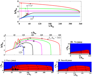
Influence of channel downslope for $L_{c}/h_{in}=360$. Panels (a) and (b) denote respectively the free surface profiles obtained from shallow water theory and numerical simulation while (c) displays simulated values of local $Fr_{m}$. In (a), the red, green, magenta, black, cyan and blue curves correspond to $\unicode[STIX]{x1D703}=0^{\circ }$, $0.6^{\circ }$, $1.5^{\circ }$, $2.1^{\circ }$, $5^{\circ }$ and $10^{\circ }$ respectively for $Re=75$. In (b,c), the red, green, magenta, black and blue curves correspond to $\unicode[STIX]{x1D703}=0^{\circ }$, $0.3^{\circ }$, $0.6^{\circ }$, $0.9^{\circ }$ and $1.2^{\circ }$ respectively for $Re=100$. W, S and N marked in (b) denote wavy, smooth and no jump conditions respectively.

7.1 Influence on downstream free surface profile

An increase in upslope tilt ($-\unicode[STIX]{x1D703}$) shifts the jump upstream and increases the jump strength and free surface undulations. This is because upflow against gravity leads to rapid loss of energy and induces an early jump. Laminar dissipation also leads to repeated undulations of high amplitude and increased vorticities underneath the undulations, as is evident from the streamline patterns in figure 12. Interestingly, beyond a critical channel tilt, the jump condition (2.18) is not satisfied by upstream and downstream conditions. This indicates that, even at high Reynolds numbers, although the incoming flow is supercritical the flow throughout the channel is subcritical, a situation akin to a submerged jump condition.

As expected, the reverse phenomenon occurs for downslope flow. With an increase in inclination, the jump shifts downstream and gradually disappears. Shallow water theory further predicts that, for sufficiently high downward inclination when the jump disappears, the free surface height, obtained from the upstream solution, initially increases along the axial distance and eventually becomes constant without exhibiting a discontinuity (black, cyan and blue curves in figure 13a). The constant height ($h_{0}$) decreases monotonically with increasing channel inclination. Figure 14 further shows that the constant height during supercritical flow throughout the channel can be obtained from the exact analytical solution (Ruschak et al. Reference Ruschak, Weinstein and Ng2001) of the Navier–Stokes equation for fully developed free falling films

(7.1)$$\begin{eqnarray}h_{0}=\left(\frac{3\unicode[STIX]{x1D708}_{l}q}{g\sin \unicode[STIX]{x1D703}}\right)^{1/3}.\end{eqnarray}$$

The observations thus demonstrate that shallow water theory can capture the effect of channel inclination over the entire zone of laminar jump formation and can also predict the range of inclinations where jump occurs.

An increase in channel length displays an effect similar to a decrease in channel inclination. The jump shifts upstream and increases its strength and undulations for longer channels, thus changing the flow from wavy to smooth and no jump conditions with a decrease in $L_{c}/h_{in}$ (figure 15). This is an expected outcome as an increased channel length increases viscous flow dissipation and hinders the liquid in continuing its rapid motion. A similar effect has also been reported by Dasgupta et al. (Reference Dasgupta, Tomar and Govindarajan2015) for an increasing height of the obstacle placed after the jump. However, the authors had noted that an increase of obstacle height beyond a critical value removes the possibility of attaining steady state since the undulations develop steeper fronts and eventually break. On the other hand, in our simulations, such an unsteady process is not encountered for either increasing channel length or increasing upward inclination.

The variation of the downstream free surface profile with $Re$ (figure 16) is as expected. In a horizontal channel, for very low Reynolds number (red curves in figure 16a), a submerged jump occurs and, on increasing the Reynolds number, the jump shifts downstream from the inlet.

Figure 14.

Constant liquid heights for $Re=75$ under no jump condition as obtained from shallow water theory (red circles) and exact solution (7.1) of the Navier–Stokes equations for fully developed free falling film.

7.2 Influence on upstream free surface profile

Unlike the downstream profile, the upstream free surface profile is independent of both channel inclination and channel length and is influenced by $Re$ only. The effect of varying the channel length can be regarded as equivalent to a variation of the downstream boundary condition and so this is an expected outcome as the information of changes in the downstream boundary condition cannot propagate across the jump to the upstream supercritical flow. On the contrary, the influence of channel tilt appears to be counterintuitive since the flow encounters the change in slope right from the entry. To ascertain this observation, we have extended our investigations to $\unicode[STIX]{x1D703}=30^{\circ }$. Figure 13(a) reveals that even for higher $\unicode[STIX]{x1D703}$, the increasing height profile, no jump condition coincides with the upstream free surface profile when a jump occurs. However, further investigations are required when turbulent flow or a wavy free surface comes into the picture.

To summarize, the observations demonstrate that, while flow variables influence the hydrodynamics both before and after the jump, the geometric variables appear to influence the flow downstream of the jump only.

Figure 15.

Influence of channel length on free surface profiles as obtained from (a) shallow water theory and (b) numerical simulations. Numerical results of (c) local $Fr_{m}$ and (d) streamline patterns for flow conditions I, II and III denoted in (b). In (a), the red, black and blue curves correspond to $L_{c}/h_{in}=360$, 240 and 120 respectively for $Re=75$. In (b,c), the red, green, magenta, black and blue curves correspond to $L_{c}/h_{in}=360$, 300, 240, 180 and 120 respectively for $Re=100$. W, S and N marked in (b) denote wavy, smooth and no jump conditions respectively.

A comparison of Froude number for circular and planar hydraulic jumps reveals a fascinating trend. We note that in the case of a circular hydraulic jump on a horizontal plane, different researchers have reported conflicting trends of Froude number measured just after the jump. Duchesne et al. (Reference Duchesne, Lebon and Limat2014) have noted the Froude number to be locked on to a constant value independent of the flow rate, kinematic viscosity and surface tension while Mohajer & Li (Reference Mohajer and Li2015) obtained constant values of the Froude number independent of the flow rate and plate size but dependent on surface tension. The origin of the constant values is to date not fully understood. In the present case of planar laminar jumps, we observe the variation of Froude number with axial distance as a function of Reynolds number (figure 16c), channel length (figure 15c) and channel inclination for both upslope (figure 12c) and downslope (figure 13c) flows. No locking of Froude number is noted. This may be attributed to the definition of the Froude number, which for circular jumps $(Fr_{cir}=Q/(2\unicode[STIX]{x03C0}r\sqrt{gh^{3}}))$ involves two variables – the liquid height $h$ and the radial location $r$ for a given flow rate $Q$ and for planar jumps $(Fr_{m}=q/(\sqrt{gh^{3}(\cos \unicode[STIX]{x1D703}\mp \sin \unicode[STIX]{x1D703})}))$ involves only one variable – the liquid film thickness $h$ – at a given $q$ for all channel orientations (horizontal, downslope and upslope cases).

7.3 Influence on jump location

In an earlier work, Singha et al. (Reference Singha, Bhattacharjee and Ray2005) had proposed a scaling dependence of $x_{j}$ on $q^{5/3}$ for horizontal flow. In the present paper, we observe that the linearity (of $x_{j}$ as a function of $q^{5/3}$) holds for inclined channels as well (figure 17) in the present range of investigation ($-0.6^{\circ }\leqslant \unicode[STIX]{x1D703}\leqslant 0.6^{\circ }$), provided the jump is not near the exit ($x_{j}/L_{c}<\sim 0.5$). The slope of the linear fit increases with $\unicode[STIX]{x1D703}$, thus suggesting a faster downstream shift of jump position for higher $\unicode[STIX]{x1D703}$. This is probably because the increased gravitational force in the flow direction aids in countering the viscous resistance. Further, the linear fit for a particular $\unicode[STIX]{x1D703}$, when extrapolated to $x_{j}=0$, gives the condition for a submerged jump, denoted by $q=q_{0}$ in the inset of figure 17. The value of $q_{0}$ decreases as $\unicode[STIX]{x1D703}$ increases and for $q<q_{0}$, the flow is subcritical throughout the channel.

Figure 16.

Influence of Reynolds number for a constant channel length $L_{c}/h_{in}=360$. Panels (a) and (b) display the respective free surface profiles obtained from shallow water theory and numerical simulations with (c) displaying the numerical results of local $Fr_{m}$. The inset in (b) gives the magnified view of upstream free surface profiles. The horizontal dashed line in (c) represents $Fr_{m}=1$ and the vertical dashed lines indicate the location in the jump region where local $Fr_{m}$ is unity. In (a), the red, green, magenta and black curves correspond to $Re=50$, 75, 100 and 125 respectively. Red curve in (a) corresponds to submerged jump. In (b,c), the red, green, magenta and black curves correspond to $Re=100$, 125, 150 and 175 respectively. W, S and N marked in in (b) denote wavy, smooth and no jump conditions respectively.

Figure 17.

Scaling relationship of jump location with $q^{5/3}$ for different channel inclinations. Black and blue colours correspond to experimental and analytical results respectively.

It is interesting to note that, despite exhibiting a singularity at the jump region, the shallow water results (blue legends) are in close agreement with experimental data (black legends) and the consistent linearity predicted from theory is also demonstrated from experiments.

7.4 Jump types

The simulated results consolidated as a pair of phase diagrams in figure 18 display the presence of submerged, wavy, smooth and no jump conditions. As discussed above, each transition is characterized by a decrease in (i) jump strength, (ii) free surface undulations and (iii) steepness in the jump front. The transition from a wavy to a smooth jump is observed to occur at $h_{2}/h_{1}\approx 2$ and the no jump condition is characterized by $Fr_{m}>1$ throughout the flow length. In the figure, the experimental data obtained from channels of three different lengths and six different inclinations are also superimposed. A reasonable agreement between experiments and simulations is evident in both figures, barring some mismatches close to the transition boundaries. This can be attributed to experimental factors and the subjectivity in distinguishing a wavy jump and a smooth jump based on undulations of the free surface.

We observe that jumps are favoured at low $Re$, for longer channels and adverse slopes and change to smooth and no jump conditions with a gradual decrease in $L_{c}/h_{in}$ and gradual increase in $\unicode[STIX]{x1D703}$. Both simulations and experiments also indicate that, for any channel length, a jump does not form beyond a critical $Re$ whose value is less for shorter channels and no jump will occur if the channel length is smaller than a critical value. The critical channel length and critical $Re$ are thus interdependent: a higher critical $Re$ for longer channels and a lower critical length for lower flow rates (smaller $Re$ values).

Similarly, for downslope flows aided by gravity, an increase in $\unicode[STIX]{x1D703}$ causes the transformation from wavy to smooth and subsequently no jump conditions at lower $Re$. With an increase in $\unicode[STIX]{x1D703}$, the critical $Re$ for jump formation decreases and for a particular $Re$, there is a critical $\unicode[STIX]{x1D703}$ beyond which no jump is formed under the balance of gravity, inertia and viscous forces. Thus, we conclude that jump formation and its nature depend on the coupled effects of channel length, channel inclination and Reynolds number and a stronger jump can result even at higher $Re$ for a long enough channel and a large enough ($-\unicode[STIX]{x1D703}$).

Figure 18.

Phase diagram for jump type (shown schematically in c) as a function of Reynolds number and channel geometry – (a) scaled channel length and (b) channel inclination. In (a,b), curves demarcate zones of numerically simulated jump types. Hatched region shows zone of numerically simulated submerged jump.