2.1 Micromodel design and microfabrication

Figure 1 shows the full micromodel pattern: 661 cylinders of diameter  $d_{c}$ are arranged along 28 spirals and sandwiched between two plates, separated by a height  $h$ . In figure 1, the cylinders along a given spiral are marked out by an integer number between 1 and 24, with the number 1 for the most external cylinder. The centre-to-centre distances between two neighbouring cylinders along a given spiral, $w_{/\!/}$ , and between a cylinder and its closest neighbour in the adjacent spiral (in the anticlockwise direction), $w_{\bot }$ , are shown in figure 2. In this paper, we present results obtained on micromodels designed with $h=d_{c}=50~\unicode[STIX]{x03BC}\text{m}$ . Note that in order to validate the image processing algorithm used to measure the amount of liquid within a micromodel against data obtained using a balance (see § 2.3), we also had to use a larger micromodel, with $d_{c}=500~\unicode[STIX]{x03BC}\text{m}$ and $h=525~\unicode[STIX]{x03BC}\text{m}$ .

The microfabrication protocol combines the classical photolithography exposure, bake and development steps with the commonly used epoxy-based SU8 photoresist as a material. It is detailed in Chen (Reference Chen2016) and we only highlight here some of its key features. First, it is important to note that, for the large micromodel, the glass bottom plate is covered by a $10~\unicode[STIX]{x03BC}\text{m}$ thick SU8 layer, prior to the realization of the cylinders. The glass top plate is also covered by a $10~\unicode[STIX]{x03BC}\text{m}$ thick SU8 layer before bonding. Thus, all the surfaces in contact with the liquid are made of SU8; see figure 1. Second, the protocol for the small system differs from that used for the large system in one major point: the top plate consists of only a $20~\unicode[STIX]{x03BC}\text{m}$ dry epoxy film (DF1020 negative photoresist), which is laminated on top of the bottom part of the micromodel (after the pattern of cylinders has been completed). The circular shape of the top plate is obtained following a photolithography exposure, bake and development procedure, during which good alignment of the top plate is ensured (whereas it is done manually in the large micromodel). Characterization of the bottom plates of the micromodels after microfabrication by optical profilometry and scanning electron microscopy (SEM) ensured that the designed dimensions were well reproduced, typically within a few micrometres.

Figure 1.

Micromodel pattern. Top right: Along a given spiral, the centre-to-centre distance between two cylinders is denoted $w_{/\!/}$ whereas the distance between a cylinder and its closest neighbour in the adjacent spiral (in the anticlockwise direction) is denoted $w_{\bot }$ . Bottom-right: Side view of the micromodel edge, for the large micromodel with $d_{c}=500~\unicode[STIX]{x03BC}\text{m}$ and $h=525~\unicode[STIX]{x03BC}\text{m}$ . The distance between the circular top plate and the rim of the cylinder pattern is $2d_{c}$ . The SU8 photoresist appears in grey. Note that there is no glass top plate for the small micromodel ( $d_{c}=h=50~\unicode[STIX]{x03BC}\text{m}$ ): the DF1020 top film is directly laminated on the pattern of cylinders.

Figure 2.

Distance between neighbouring cylinders, $w_{/\!/}$ and $w_{\bot }$ (see figure 1), made dimensionless by dividing by twice the cylinder diameter $d_{c}$ , plotted as a function of the cylinder number along a given spiral.

2.2 Protocol for a drying experiment

The micromodel is positioned horizontally on top of a plane light-emitting diode (LED) light source (Phlox LedW-BL) and is imaged from the top by a sCMOS Lavision camera with a 2048 pixel $\times$ 2048 pixel sensor. The micromodel and LED back-light are therefore perpendicular to the optical axis. The spatial resolution is typically around 1.8 pixel per micrometre (for micromodels with $h=d_{c}=50~\unicode[STIX]{x03BC}\text{m}$ ). The images are acquired at a fixed acquisition rate, from 0.01 Hz to 100 Hz depending on the experiment. The LED light source is triggered by an external source and synchronized with image acquisition. A small droplet of the working liquid is gently deposited at the edge of the device and then fully fills the micromodel by capillary suction. Image acquisition is then immediately launched to follow the liquid evaporation. The experiments are performed in a temperature-controlled environment, with $T=22\pm 1\,^{\circ }\text{C}$ . Evaporation takes place in a stagnant and ‘dry’ air atmosphere: there is no imposed external air flow and the vapour concentration in the room is assumed to be zero.

Several liquids were used and their relevant thermophysical properties are listed in table 1. Data for dynamic viscosity $\unicode[STIX]{x1D707}_{f}$ and vapour pressure at the working temperature were obtained using tabulated values and estimating methods proposed by Reid, Prausnitz & Sherwood (Reference Reid, Prausnitz and Sherwood1987). Data for surface tension are from Jasper & Kring (Reference Jasper and Kring1955). The error bars given come from the uncertainty on the working temperature, $\pm 1\,^{\circ }\text{C}$ . Data for the vapour–air diffusion coefficient $D$ were obtained from various references (Cummings & Ubbelohde Reference Cummings and Ubbelohde1953; Altshuller & Cohen Reference Altshuller and Cohen1960; Lugg Reference Lugg1968; Elliott & Watts Reference Elliott and Watts1972; Beverley, Clint & Fletcher Reference Beverley, Clint and Fletcher1999) and extrapolated to $22\pm 1\,^{\circ }\text{C}$ using expressions for temperature corrections found in Vargaftik (Reference Vargaftik1975). The uncertainties on $D$ indicated in table 1 were estimated from the scatter in the available data. All these liquids perfectly wet SU8 and DF1020: when a drop is deposited on a flat SU8 or DF1020 substrate, the liquid fully spreads, rendering any measurement of the contact angle unfeasible. In the following, the contact angle will therefore be assumed to be zero.

Figure 3.

Typical image of a micromodel. (a) Raw image, for a micromodel filled with heptane, with a resolution of 1.8 pixel per micrometre. (b) Zoom on the region of interest delimited by a dotted rectangle in panel (a). (c) Binarized image. (d) Binarized image after filling of the central liquid cluster.

Table 1.

Working liquid properties at $22\,^{\circ }\text{C}$ : $\unicode[STIX]{x1D70C}_{f}$ , $\unicode[STIX]{x1D707}_{f}$ , $\unicode[STIX]{x1D6FE}$ and $D$ correspond to liquid mass density, dynamic viscosity, surface tension and vapour diffusion coefficient in air, respectively.

2.3 Image processing

In the present study, all the relevant experimental data (i.e. evaporation rates, phase distribution and liquid film extent) were obtained by image processing. A typical image obtained with the CCD camera is shown in figure 3(a). The meniscus surrounding the central liquid cluster deviates the almost parallel light coming from the back-light and appears as the darkest region on such an image. This is better seen in the close-up on the region of interest delimited by the dotted rectangle in figure 3(a), see figure 3(b), where the cylinders embedded in the liquid cluster can also be seen. The very good spatial resolution and the wide dynamic range of such images allow us to perform quantitative measurements at the scale of the cylinders, e.g. regarding the width of the liquid bridges connecting two neighbouring cylinders, along a spiral.

The volume of liquid contained within the micromodel can be measured by image processing, at any time of the drying experiment, as explained in the following. The contrast between the dark meniscus region and the bulk fluid regions (liquid or air) is large enough so that applying a binarization operation is straightforward, leading to the image shown in figure 3(c), which is then filled, figure 3(d). On such an image, the total area of the white region, $A$ , can be readily obtained by image processing (using the Matlab regionprops built-in function). Similarly, one can detect any cylinder that is no longer wetted by the liquid and thus appears as an isolated disk. Knowing the total number of cylinders, one can have a first estimate of the liquid volume  $V$ in the micromodel, $V=Ah-N_{w}V_{p}$ , where $N_{w}$ is the measured number of cylinders embedded in the liquid cluster and $V_{p}=\unicode[STIX]{x03C0}hd_{c}^{2}/4$ is the volume of a cylinder. Then, one has to note that the white region of area  $A$ seen in figure 3(c) takes into account the projected area of the meniscus. This latter area, $A_{m}$ , can be obtained from the image shown in figure 3(b), before the filling operation is applied. In the meniscus region, the liquid is not present over the full height $h$ of the micromodel and this has to be taken into account. In fact, the formula above giving $V$ overestimates the liquid volume, whereas the alternative expression $V=(A-A_{m})h-N_{w}V_{p}$ underestimates it.

To estimate the amount of liquid in the meniscus region, we used the Surface Evolver software (Brakke Reference Brakke1992) to simulate the capillary shape of a static liquid bridge located in between two cylinders, confined between two horizontal plates. Starting from an initial ‘guess’ shape for the static liquid bridge, Surface Evolver progressively converges towards the meniscus shape by minimizing the surface energy, given a set of constraints (e.g. contact angle on solid surface and liquid volume). During the evolution procedure, the surface can be progressively refined by the user, by increasing the number of facets that shape it. In the present study, shape convergence was typically considered to be reached when the surface energy varied by less than 0.2 % between two successive surface evolution steps, its value being at the same time ‘robust’ to operations like surface refinement, vertices averaging, etc. Let us consider a typical liquid bridge shape, as shown in figure 4. We introduce $\unicode[STIX]{x1D706}$ such that the liquid content in the meniscus region is $\unicode[STIX]{x1D706}\times A_{p}h$ , where $A_{p}$ is the projected meniscus area in the $z=0$ plane. The coefficient $\unicode[STIX]{x1D706}$ can be computed from liquid bridge shapes obtained by Surface Evolver simulations. It depends on the spacing $w_{/\!/}$ between the cylinders, on the liquid volume trapped in the liquid bridge and on the contact angle. The values obtained for $\unicode[STIX]{x1D706}$ typically range between 0.13 and 0.2. In the following, we assume that the volume of liquid $V$ in the micromodel can be obtained as $Ah-(1-\unicode[STIX]{x1D706})A_{m}h-N_{w}V_{p}$ , where $A$ , $A_{m}$ and $N_{w}$ are obtained by image processing as explained above, and taking $\unicode[STIX]{x1D706}$ equal to a single typical value of 0.16. This comes down to assuming that the liquid content in the meniscus region can be estimated by determining $\unicode[STIX]{x1D706}$ on the similar, but simpler, liquid bridge geometry shown in figure 4.

Figure 4.

Typical liquid bridge capillary shape obtained from Surface Evolver. The liquid bridge is trapped between two cylinders and confined between two flat surfaces located in the $z=0$ and $z=h$ planes (not displayed). The two cylinders, of diameter $d_{c}$ , appear in light grey and are separated by $w_{/\!/}$ (here, $w_{/\!/}=d_{c}$ ). The contact angle between the liquid and the solid surfaces is $0^{\circ }$ .

This image processing-based technique for measuring the liquid content in the micromodel was validated against mass measurements performed with a Mettler-Toledo MS603S balance with a $\pm 0.001~\text{g}$ accuracy. Such a validation test was performed with the large micromodel only ( $h=525~\unicode[STIX]{x03BC}\text{m}$ ) for which the mass of liquid is around 0.3 g at the beginning of an experiment whereas it is three orders of magnitude smaller, well below the scale minimum weight limit, in the micromodels with $h=50~\unicode[STIX]{x03BC}\text{m}$ used in the drying experiments. Figure 5 compares the mass data from the balance (squares) to those obtained by image processing (after multiplying the measured liquid volume by the liquid mass density). Crosses show the data obtained when the amount of liquid in the meniscus region is neglected ( $\unicode[STIX]{x1D706}=1$ ), whereas dots show the data corrected taking $\unicode[STIX]{x1D706}=0.16$ . The latter match nicely the data obtained from the balance. Note that taking $\unicode[STIX]{x1D706}=0.13$ or 0.19 results, at most, in a negligible 2.5 % variation of the mass obtained by image processing.

Figure 5.

Mass loss during evaporation of heptane in a large micromodel ( $h=525~\unicode[STIX]{x03BC}\text{m}$ ). Squares, data from a precision balance. Crosses, respectively dots: data from liquid volume measurements by image processing with $\unicode[STIX]{x1D706}=1$ (no liquid in the meniscus region), respectively $\unicode[STIX]{x1D706}=0.16$ .

3.1 Phase distribution and evaporation rate as a function of time

Figure 6 shows the liquid–gas distribution at four successive times, $t=0$ (beginning of the experiment), $t=18~\text{s}$ , $t=62~\text{s}$ and $t=125~\text{s}$ , for evaporation of heptane. The experiment starting time, $t=0$ , is taken when the meniscus is fully positioned around the external end of the pattern, see figure 6(a). From $t=0$ to $t=18~\text{s}$ approximately, one can observe a progressive invasion of air between the spirals. Concomitantly with the gas-phase ingress, some elongated liquid films remain trapped along each spiral. In fact, the distances $w_{/\!/}$ between two cylinders along a spiral are typically small enough to allow for coalescence between the liquid clusters left around each cylinder following air invasion, liquid clusters that would otherwise remain isolated (Chen et al. Reference Chen, Duru, Joseph, Geoffroy and Prat2017). A liquid film can be described as a chain of liquid bridges between neighbouring cylinders, which first extends up to the spiral’s most external cylinder (see figure 6 b). At longer times ( $t>18~\text{s}$ ), the elongated films start to recede in the system. This is caused by successive break-ups of the most external liquid bridge of each elongated film. Thus, an elongated liquid film ‘depins’ progressively from each cylinder of the spiral, while the gas-phase ingress continues. This invasion process is described in more detail in the next subsection.

The evaporation rate, $E=-\text{d}V/\text{d}t$ , where $V$ is the liquid volume measured by image processing as described earlier, is shown in figure 7. A quasi-constant-evaporation-rate period (CRP) is observed with $E_{CRP}\approx 4.5\times 10^{-3}~\unicode[STIX]{x03BC}\text{l}~\text{s}^{-1}$ , from $t=0$ to $t=18~\text{s}$ . Once the elongated liquid films start to depin from the outermost cylinders, around $t=18~\text{s}$ , a sharp decrease of the evaporation rate is observed. The phenomenology discussed above is observed for all the liquids used. It is similar to that obtained during the drying of capillary porous media and of square cross-section capillary tubes initially filled with a volatile liquid, as discussed in the introduction (§ 1).

Figure 6.

Evaporation of heptane in a $50~\unicode[STIX]{x03BC}\text{m}$ thick micromodel: phase distribution at $t=0~\text{s}$ (a), $t=18~\text{s}$ (b), $t=62~\text{s}$ (c) and $t=125~\text{s}$ (d).

Figure 7.

Evaporation of heptane in a $50~\unicode[STIX]{x03BC}\text{m}$ thick micromodel: evaporation rate $E$ (in  $\unicode[STIX]{x03BC}\text{l}~\text{s}^{-1}$ ) as a function of time.

3.2 Phase distribution evolution at pore scale: an invasion process

To describe the phase distribution at pore scale, we will describe a given liquid film as a chain of connected liquid bridges, positioned between each pair of neighbouring pillars along a spiral. Then, the space between two spirals will be described as a succession of pores, each pore throat being located in between pairs of neighbouring pillars in adjacent spirals. Each liquid film will be marked out using the number of the most external cylinder wetted by the liquid and connected to the main, central liquid cluster, i.e. using a number between 1 and 23. Similarly, each main meniscus location within the micromodel will be marked out by the number of the pore it occupies. A sketch detailing these conventions is shown in figure 8(a). Note that such a representation allows us to compare readily experiments performed with different liquids, even if the experiment duration changes a lot from one liquid to another, depending on the liquid volatility.

In figure 8(b), the location of the film end (i.e. the location the external tip of the chain of liquid bridges forming the film) is plotted as a function of the main meniscus location for a given ‘pair’ of liquid film and main meniscus, in an experiment performed using heptane as evaporating liquid. For each recorded image, these two locations are determined by image processing. Film and main meniscus locations only take integer values between 1 and 23, see open circles in figure 8(b). The data points corresponding to the beginning of the experiments are in the lower left corner of the graph. As both film end and main meniscus recede towards the micromodel centre with time, they are both marked out by larger and larger numbers.

Figure 8.

(a) Sketch showing the way the locations of the main menisci and the liquid films are marked out. As an example, for the three spiral ends seen in this close-up of the micromodel, the liquid film location is at cylinder #2. Two main menisci at location #7 are also highlighted by an arrow. (b) Liquid film end location as a function of the main meniscus location, for a drying experiment performed with heptane. Open circles and dotted line: data for a given liquid film–main meniscus pair. The filled black circle highlighted by an arrow marks out the data point corresponding to the particular situation depicted in (a). Solid line: data averaged over the 28 liquid film–main meniscus pairs of the micromodel. The error bars show the standard deviations of the mean values of liquid film ends and main menisci locations.

It is important to note that both locations evolve in a discontinuous manner. First, the main meniscus ‘jumps’ from one pore entrance to the next. This motion is a simplified version of the so-called Haines jumps observed in more realistic porous media (see e.g. Berg et al. Reference Berg, Ott, Klapp, Schwing, Neiteler, Brussee, Makurat, Leu, Enzmann and Schwarz2013; Singh et al. Reference Singh, Scholl, Brinkmann, Di Michiel, Scheel, Herminghaus and Seemann2017b ). As an example, the displacement of a given main meniscus was extracted from a stack of images taken at a high acquisition rate (100 Hz). Figure 9 shows the meniscus curvilinear coordinate along the dotted white line seen on the two insets, as a function of time. It is clearly seen that the invasion proceeds by successive jumps: the main meniscus, positioned at the entrance of a given pore, first slowly penetrates into the pore before a sudden jump occurs and drives the main meniscus to its next position, at the entrance of the next pore. In figure 9, the two insets display the images taken just after a jump (at $t=1.23~\text{s}$ ) and just before the next one (at $t=2.1~\text{s}$ ). Second, the location of the film end is controlled by successive break-ups of the most external liquid bridge of the chain of liquid bridges forming the film. As an example, the width of the most external liquid bridge along a film is plotted as a function of time in figure 10: it decreases continuously with time until the break-up suddenly occurs, between $t=25$ and $t=26~\text{s}$ . Studying in detail the dynamics of the non-local fluid redistribution within the liquid cluster following a pore invasion or of the liquid bridge break-up is not within the scope of the present study. Such topics have been considered in recent studies, using micromodels (Armstrong & Berg Reference Armstrong and Berg2013) or packing of beads (Singh et al. Reference Singh, Menke, Andrew, Lin, Rau, Blunt and Bijeljic2017a ).

Figure 9.

Displacement of a given main meniscus as a function of time. The length $D$ is the interface curvilinear coordinate along the white dotted line shown on the insets (the origin $D=0$ being taken at the cross-marked, left end of the dotted line). The left inset shows the meniscus location just after its jump at the pore entrance at which it is located. The right inset shows the main meniscus location just before its next jump. On the two insets, the circle in white is the circle inscribed between the two pillars that mark the entrance of the pore about to be invaded.

On figure 8(b), the solid line shows the evolution of the liquid film ends as a function of the main menisci locations, averaged over the 28 spirals of the micromodel (so 28 liquid film–main meniscus pairs). A data point is obtained for each recorded image and, due to averaging, non-integer values are obtained, the error bars being taken as the standard deviations of the means. The constant-evaporation-rate period seen in figure 7 corresponds to the period during which the liquid films are connected to the spiral end, i.e. to cylinder #1. As can be seen in figure 6(b), there are some slight differences from one spiral to another, as far as the main meniscus locations are concerned and also regarding the most external cylinders wetted by the liquid. Such slight discrepancies, at a given time, from one liquid film–main meniscus pair to another, can be appreciated owing to the error bars shown in figure 8(b), for a limited set of data points (for the sake of clarity). Note that, while the amplitude of the error bars is roughly constant during a first stage for which the main menisci locations are in the range [6–12], it decreases noticeably as the liquid cluster becomes more confined in the micromodel centre (note the smaller error bars for main menisci location beyond 13). Also, it is important to state that such error bars do not come from the fact that the invasion pattern is slightly out of phase from one spiral to another but really from small differences in the invasion pattern itself, i.e. on the exact succession of main menisci and film tip locations.

3.3 Experimental results for the different liquids used

In figure 11, results using averaged values are shown for the various liquids used in the present study. All the curves display the same typical shape. First, the main menisci recede while the tips of the elongated films remain pinned to the most external cylinder (liquid film location value is then 1). Depinning from the most external cylinder occurs earlier (in terms of main meniscus location) for the most volatile fluids or, equivalently, for the highest capillary numbers (see below). The differences between one liquid and another become less pronounced when the liquid cluster is confined in the centre of the micromodel (typically for main meniscus locations larger than #17 and film locations larger than #7). Note that drying experiments were repeated several times (3–5 times) for each liquid with a very good reproducibility: one can hardly discern any differences from one experiment to another when their results are plotted on the same graph. Therefore, the slight difference seen in figure 11 between heptane and hexane is significant: on average, the first liquid bridge break-up occurs earlier with hexane (dots) than with heptane (crosses) and the liquid films observed with hexane are typically one liquid bridge shorter than with heptane, during most of the experiment duration.

Figure 10.

Break-up of a liquid bridge (fluid: heptane). The liquid bridge width $w$ , measured along the dotted line shown in the top-left inset, made dimensionless by its initial value $w_{i}$ , is shown as a function of time. The insets display the liquid bridge as seen on the images. The break-up occurs between $t=25$ and $t=26~\text{s}$ and $w/w_{i}$ falls to 0. After the break-up, the presence of isolated liquid rings around the external cylinder base and top is demonstrated by the sharp black ring around the cylinder. Such an optical signature of the liquid rings disappears as the liquid contained in the rings evaporates (see image at $t=27~\text{s}$ ).

Figure 11.

Drying experiments: averaged location of the liquid film ends as a function of the averaged location of the main menisci, for the various liquids used (see legend for details). The three insets display the phase distribution just before depinning, and thus at maximal film extent, for hexane, octane and decane.

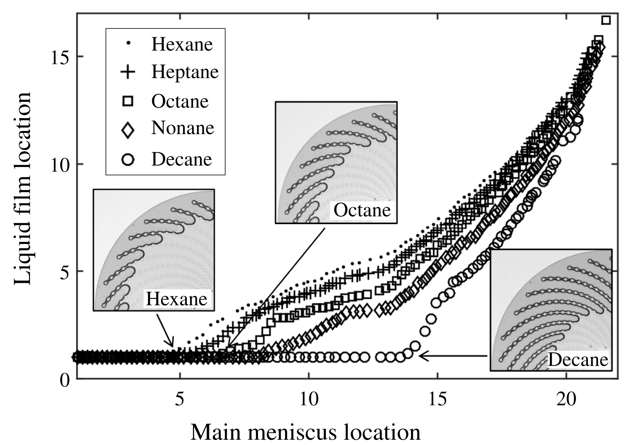
Table 2 recapitulates the results obtained for the several liquids used, regarding the evaporation rate measured during the CRP, $E_{CRP}$ , the capillary number $Ca$ (introduced and discussed in § 4.2), and the liquid film length evolution during drying. Table 2 gives the averaged main meniscus locations when depinning occurs from cylinder #1 and #4, denoted $L_{1}$ and $L_{4}$ respectively. In the next section, the emphasis will be on the understanding of the liquid film dynamics, i.e. on the prediction of the typical curve shape displayed in figure 11, including $L_{1}$ and $L_{4}$ values. The values of $E_{CRP}$ are discussed in Chen et al. (Reference Chen, Duru, Joseph, Geoffroy and Prat2017).

Table 2.

Experimental results: evaporation rate during the CRP ( $E_{CRP}$ ), capillary number $Ca$ as defined by (4.5) in § 4.2, mean main meniscus locations at depinning from the most external cylinder (#1), $L_{1}$ , and mean main meniscus locations when the films depin from cylinder #4, $L_{4}$ . The uncertainty is taken as the standard deviation to the mean obtained when averaging data from several experiments, performed with a given liquid.

4.1 Critical capillary pressure of a liquid bridge and pore invasion pressure

A key point of the above scenario is that there is a critical capillary pressure (or equivalently critical curvature) above which a liquid bridge cannot be sustained in between two neighbouring cylinders. This point was studied using the software Surface Evolver (SE), by simulating the shape of single liquid bridges trapped between two cylinders, confined between two horizontal plates. Such liquid bridges can be considered as the building block of the elongated liquid films that are observed along each spiral in the experiment. Typically, for a given spacing between the two cylinders, a converged liquid bridge shape was computed as a function of the liquid volume. The equilibrium capillary pressure and relevant geometrical parameters describing the liquid bridge were obtained for each volume step. We assume that the liquid bridge break-up occurs when its thickness $t$ at the location $(x=0,y=w_{/\!/}/2,z=h/2)$ , see figure 4, tends to zero (simulations are typically stopped when $t/2d_{c}=0.01$ ). The critical pressure for a liquid bridge is then that obtained in SE ‘just before’ the two liquid–gas interfaces collapse. Figure 12 shows the evolution of the dimensionless critical pressure, $2d_{c}\times P_{crit}/\unicode[STIX]{x1D6FE}$ , obtained in SE for a zero contact angle, as a function of the dimensionless spacing between the two cylinders, $w_{/\!/}/2d_{c}$ . As expected, the critical pressure increases when $w_{/\!/}$ decreases. Results for different contact angles and details in the use of SE are given in Chen (Reference Chen2016).

Figure 12.

Critical capillary pressure for liquid bridge break-up. The capillary pressure $P_{gas}-P_{liquid}$ is made dimensionless by dividing by $\unicode[STIX]{x1D6FE}/2d_{c}$ and is plotted as a function of the dimensionless centre-to-centre distance between the two cylinders, $w_{/\!/}/2d_{c}$ . The contact angle of the liquid on the cylinders and on the top and bottom plates is zero.

In the experiment, the elongated liquid films observed consist of chains of connected liquid bridges and break-up occurs systematically for the most external liquid bridge. To check if the critical capillary pressure obtained for an isolated liquid bridge is a fair approximation of the critical pressure at play in the experiment, some SE simulations were also ran along a chain of cylinders with varying distances between the cylinders, corresponding to those imposed by the microfabrication design. Capillary shapes of elongated films were obtained for successive, decreasing liquid volumes until the liquid bridge break-up occurs in between the two most distant cylinders. The critical pressure found when considering a chain of $N$ cylinders (i.e. $N-1$ liquid bridges), made dimensionless by its value for $N=2$ , was found to vary by less than 1 %, whatever $N$ is, compared to the reference case ( $N=2$ ).

Another key element of the basic invasion mechanism outlined above is the knowledge of the capillary pressure to be reached to invade a given pore, $P_{inv,i}$ . As seen in figure 10, the liquid–gas interface just before invasion of pore # $i$ closely matches the circle inscribed in between the two pillars highlighted in red, i.e. the opening of the pore about to be invaded. Such an observation was repeated over several invasion events. Consequently, the invasion capillary pressure for a given pore # $i$ is estimated as

(4.1) $$\begin{eqnarray}P_{inv,i}=\unicode[STIX]{x1D6FE}\left(\frac{2}{D_{i}}+\frac{2}{h}\right),\end{eqnarray}$$

where $2/D_{i}$ is the curvature of the interface in the observation plane with $D_{i}=w_{\bot ,i}-d_{c}$ , $h$ is the micromodel thickness and the liquid is perfectly wetting (zero contact angle). Note that $D_{i}$ is a function of the pore considered and decreases as one penetrates further into the micromodel.

4.2 Viscous pressure drop within the liquid films

To estimate the viscous pressure drop due to the evaporation-induced flow within the liquid films, we again regard the liquid film as a succession of connected liquid bridges. A pressure drop $\unicode[STIX]{x0394}P_{\unicode[STIX]{x1D707},i}$ is defined for each liquid bridge  $i$ (located between cylinders  $i$ and  $i+1$ ) as the flow-induced pressure difference between the liquid bridge inlet and outlet, located in planes $y=0$ and $y=w_{i}$ respectively, see figure 4. The invasion algorithm in a viscocapillary case, described in the next subsection, will require an estimate of the pressure in the middle of each liquid bridge  $i$ , for a given position  $j$ of the main meniscus:

(4.2) $$\begin{eqnarray}P_{lb,i}=P_{inv,j}-\left(\frac{\unicode[STIX]{x0394}P_{\unicode[STIX]{x1D707},i}}{2}+\mathop{\sum }_{k=i+1}^{k=j-1}\unicode[STIX]{x0394}P_{\unicode[STIX]{x1D707},k}\right).\end{eqnarray}$$

To calculate $\unicode[STIX]{x0394}P_{\unicode[STIX]{x1D707},i}$ , we follow the classical analysis of Ransohoff & Radke (Reference Ransohoff and Radke1988) for corner flows, which relates the pressure drop to the flow rate in the liquid film by a Poiseuille-like law:

(4.3) $$\begin{eqnarray}\unicode[STIX]{x0394}P_{\unicode[STIX]{x1D707},i}=\frac{\unicode[STIX]{x1D6FD}}{R_{in,i}^{2}}\unicode[STIX]{x1D707}_{f}w_{/\!/,i}\frac{q_{i}}{A_{in,i}}.\end{eqnarray}$$

In this expression, $q_{i}$ is the liquid flow rate in the liquid bridge, $A_{in,i}$ is the liquid bridge total cross-section area in the $y=0$ plane and $\unicode[STIX]{x1D6FD}$ is a dimensionless flow resistance, which is a function of the liquid bridge shape, the contact angle and the boundary condition at the liquid–air interface. In the $y=0$ plane, the liquid bridge consists of four identical liquid corners/wedges, confined between the horizontal plates and the cylinder wall, with a radius of curvature $R_{in,i}$ in the plane $y=0$ .

Use of (4.3) requires the knowledge of the liquid bridge shape ( $A_{in}$ and $R_{in}$ ), of the viscous resistance $\unicode[STIX]{x1D6FD}$ , and of the liquid flow rate within the liquid bridge. An extensive set of SE simulations of liquid bridges was first performed, giving $A_{in}$ and $R_{in}$ as a function of the capillary pressure and $w_{/\!/}$ . The viscous resistance $\unicode[STIX]{x1D6FD}$ was then obtained from direct numerical simulations (DNS) of the flow within the simulated liquid bridges (the detailed procedure and validation tests are presented in appendix A).

Therefore, in the present modelling, the viscous flow-induced pressure drop within each liquid bridge is computed using a liquid bridge shape obtained at capillary equilibrium (i.e. with no flow). As the capillary number is small in the present experiments, deviations from the capillary shape should be small and the present local equilibrium assumption is expected to be relevant. Note that avoiding such an assumption would require one to simulate the flow within the film together with the film shape, using a volume-of-fluids (VOF) or a level-set method, for instance. However, such numerical techniques remain numerically challenging and computationally demanding in the case of low-capillary-number flows, e.g. due to spurious effects such as parasitic currents (Horgue et al. Reference Horgue, Augier, Quintard and Prat2012; Raeini, Blunt & Bijeljic Reference Raeini, Blunt and Bijeljic2012). Use of DNS techniques allowing interface tracking in the present film flow problem is then well beyond the scope of the present paper.

As far as the flow rate within the liquid bridge is concerned, we assume that the pore space remains saturated with vapour during the micromodel drying, due to confinement effects. Such an assumption has been validated by simulations of the stationary vapour concentration field in the pore space (see Chen Reference Chen2016). As a result, evaporation occurs at the tip of the liquid films only, i.e. around the last cylinder connected to the liquid film, and the flow rate $q$ is constant along a liquid film. We also assume that the evaporation rate is evenly distributed around the 28 spirals of the system so that $q=E/28$ . The evaporation rate $E$ is measured experimentally, as explained earlier, and its evolution during a drying experiment can be formulated as a function of the location of the liquid film tips: $E=E_{\text{CRP}}\times f_{i}$ , where $i$ is the film tip location (i.e. the number of the most external cylinder wetted by the liquid films, averaged over the 28 liquid films). The function $f_{i}$ is such that $f_{1}=1$ and can be obtained experimentally. It is well fitted by an fifth-order polynomial and does not depend on the liquid used.

Finally, (4.3) can be manipulated to introduce the relevant, dimensionless capillary number. To that end, we introduce $R_{0}$ , a typical order of magnitude for $R_{in}$ , such that $R_{in}/R_{0}\approx O(1)$ for all the liquid bridge geometries relevant in the present study. Then,

(4.4) $$\begin{eqnarray}\frac{\unicode[STIX]{x0394}P_{\unicode[STIX]{x1D707}}}{\unicode[STIX]{x1D6FE}}=\frac{\unicode[STIX]{x1D707}}{\unicode[STIX]{x1D6FE}}\frac{\unicode[STIX]{x1D6FD}E_{CRP}fw_{/\!/}}{28\times A_{in}\times R_{in}^{2}}=\frac{\unicode[STIX]{x1D707}}{\unicode[STIX]{x1D6FE}}\frac{E_{CRP}}{28\times R_{0}^{2}}\times \frac{\unicode[STIX]{x1D6FD}fw_{/\!/}R_{0}^{2}}{A_{in}R_{in}^{2}}=Ca\unicode[STIX]{x1D6FD}\frac{fw_{/\!/}R_{0}^{2}}{A_{in}R_{in}^{2}},\end{eqnarray}$$

where the capillary number $Ca$ is defined as

(4.5) $$\begin{eqnarray}Ca=\frac{\unicode[STIX]{x1D707}}{\unicode[STIX]{x1D6FE}}\frac{E_{CRP}}{28R_{0}^{2}}\end{eqnarray}$$

and can be calculated taking $R_{0}=10~\unicode[STIX]{x03BC}\text{m}$ , see table 2. Note that a Reynolds number for the liquid flow within the liquid films can be defined as $Re=\unicode[STIX]{x1D70C}_{f}uR_{0}/\unicode[STIX]{x1D707}_{f}$ , with $u\approx E_{CRP}/(28R_{0}^{2})$ . Such a Reynolds number is in the range $O(10^{-3}){-}O(0.1)$ in the experiments.

4.3 Invasion algorithms and comparison between theoretical predictions and experimental results

Once $P_{inv}$ and $P_{crit}$ are estimated, the expected invasion pattern in the capillary case, $Ca=0$ , is obtained straightforwardly. For given locations $(i,j)$ of the liquid film tip and main meniscus, respectively (initialization is at $i=1$ , $j=2$ ), one compares $P_{inv,j}$ and $P_{crit,i}$ . If $P_{inv,j}<P_{crit,i}$ , $j\rightarrow j+1$ , otherwise break-up occurs and $i\rightarrow i+1$ . When the capillary number is non-zero, one first needs to compute the liquid pressure distribution along the liquid film. Then, the pressure in the middle of the most external liquid bridge is compared to $P_{crit}$ . More precisely, the viscocapillary algorithm is the following.

1. (i) The pressure at the liquid bridge $j-1$ , $P_{lb,j-1}$ , is initialized at $P_{inv,j}$ . The radius of curvature $R_{in,j-1}$ is obtained by extrapolating from the set of SE simulation data, giving $R_{in,j-1}$ as a function of $P_{lb,j-1}$ . The dimensionless evaporation rate is set to $f_{\#j}$ . The pressure drop $\unicode[STIX]{x0394}P_{\unicode[STIX]{x1D707},j-1}$ is then computed using (4.3).

2. (ii) The pressure at the liquid bridge is then set to $P_{inv,j}-\unicode[STIX]{x0394}P_{\unicode[STIX]{x1D707},j-1}/2$ . This new pressure involves a new liquid bridge shape and so an updated radius of curvature $R_{in,j-1}$ is obtained to compute a new $\unicode[STIX]{x0394}P_{\unicode[STIX]{x1D707},j-1}$ . A few iterations are needed for this procedure to converge to stable values for $\unicode[STIX]{x0394}P_{\unicode[STIX]{x1D707},j-1}$ and $P_{lb,j-1}$ . Then, liquid bridge $j-2$ is considered: $P_{lb,j-2}$ is initialized at $P_{inv,j}-\unicode[STIX]{x0394}P_{\unicode[STIX]{x1D707},j-1}$ and the above procedure is repeated until convergence for $\unicode[STIX]{x0394}P_{\unicode[STIX]{x1D707},j-2}$ and $P_{lb,j-2}$ .

3. (iii) Once the pressure drops have been obtained for all the liquid bridges, the pressure $P_{lb,i}$ computed from (4.2) is compared to $P_{crit,i}$ . If smaller, the main meniscus recedes, $j\rightarrow j+1$ . Otherwise, break-up occurs. In this case, the film length is set to be one liquid bridge shorter, $i\rightarrow i+1$ . In both cases, the full algorithm is repeated from step (i) above, to identify the next step of the invasion process (pore invasion or liquid bridge break-up), and so on.

The prediction of the capillary model ( $Ca=0$ ) is shown as open circles in figure 13 together with results obtained taking into account viscous effects, for $Ca=10^{-5}$ , $3.18\times 10^{-5}$ and $2\times 10^{-4}$ , shown as squares, diamonds and crosses, respectively, in figure 13. For sufficiently ‘large’ capillary numbers, typically $Ca>10^{-6}$ , deviations from the capillary curve are found. The trend observed as capillary numbers increase is the same as in the experiments, see figure 11. When the capillary number is large, $Ca>3\times 10^{-4}$ , no films are formed during the early invasion process. From initialization at $i=1$ and $j=2$ , the system directly jumps to $i=2$ and $j=3$ as the single liquid bridge between cylinders #1 and #2 cannot be sustained. However, the evolution does not follow the dotted line shown in figure 13, which shows the result obtained from the invasion algorithm when elongated films never develop. When the evaporation rate has decreased sufficiently, the viscous effects decrease and elongated films consisting of several connected liquid bridges can be found (as soon as the main meniscus has receded to location #6 for the $Ca=2\times 10^{-4}$ case shown in figure 13). Note, however, that such a case was not observed in the present experiments. It could probably be observed for highly volatile liquids, for which the present isothermal modelling may be inappropriate.

Figure 13.

Theoretical predictions regarding the liquid film end location as a function of the main meniscus location for four different capillary numbers (see legend for details). The solid line is the result obtained for drying experiment performed with heptane at $Ca=3.18\times 10^{-5}$ , see table 2 and figure 8(b). The straight dotted line shows the result obtained from the invasion algorithm when no films can develop, i.e. for ‘large’ capillary numbers.

A qualitative agreement between experiment and theory is shown in figure 13 for the particular case of drying with heptane, for which $Ca=3.18\times 10^{-5}$ . This remains true when considering the other liquids used in the present study (data not shown in figure 13 for the sake of clarity) and this can be appreciated in figure 14, where the main meniscus locations when depinning occurs from cylinders #1 and #4, denoted $L_{1}$ and $L_{4}$ , respectively, are plotted as a function of the capillary number $Ca$ . The theoretical prediction (squares and circles) converges to the purely capillary case as soon as $Ca<8\times 10^{-7}$ . The transition to a viscocapillary regime occurs in the range $Ca=10^{-6}-10^{-4}$ and is quite sharp. For $Ca>10^{-4}$ , the first liquid bridge cannot be sustained, as discussed above. Experimental data from table 2 are shown as crosses ( $L_{1}$ ) and dots ( $L_{4}$ ). Despite some discrepancies, the trend from the theoretical prediction is reproduced and the agreement between modelling and experiment is quite satisfactory, given the various approximations made in the modelling, notably the local capillary equilibrium assumption.

Figure 14.

Film length, expressed in number of connected liquid bridges, as a function of the capillary number $Ca$ when depinning from cylinders #1 and #4 occurs, $L_{1}$ and $L_{4}$ . Circles, respectively squares: theoretical prediction for depinning from cylinder #1, respectively #4. Crosses, respectively dots: experimental results for $L_{1}$ , respectively $L_{4}$ (see table 2).