
1. Introduction
The flow over a surface-mounted finite roughness is of considerable fundamental interest in fluid mechanics and widely encountered in numerous practical applications, such as in aerospace, water conservancy and shipbuilding. The complex coherent structures in the flow around the protrusion have a significant impact on the energy, mass and momentum transport in the flow fields. The characterisation of these vortex structures for various obstacles has proven challenging. This is because although the surface-mounted obstacle, such as a hemisphere, has a simple geometry, the flow over it is highly unsteady three-dimensionally. Downstream of the hemisphere, hairpin vortices are periodically formed and shed. It has been shown that its characteristics are very similar to the typical hairpin vortex structures generated in turbulent boundary layers (TBLs) (Zhou et al. Reference Zhou, Adrian, Balachandar and Kendall1999; Adrian et al. Reference Adrian, Meinhart and Tomkins2000; Lozano-Durán et al. Reference Lozano-Durán, Flores and Jiménez2012; Gao et al. Reference Gao, Sun, Chen, Fan and Zhang2021). Since it is difficult to accurately measure and extract individual typical hairpin vortices in a practical TBL due to the disturbance of turbulence, hemisphere protuberance is also an alternative approach to artificially generating hairpin vortices in laminar boundary layers (Acarlar & Smith Reference Acarlar and Smith1987a ; Hajimirzaie et al. Reference Hajimirzaie, Wojcik and Buchholz2012; Gao et al. Reference Gao, Sun, Chen, Fan and Zhang2021; Tu et al. Reference Tu, Wang, Gao, She, Wang, Wang and Wei2023; Qiu et al. Reference Qiu, Liu, Li, Tao and Liu2023) in addition to pulsed fluid injection (Acarlar & Smith Reference Acarlar and Smith1987b ; Svizher & Cohen Reference Svizher and Cohen2006). To this end, studying the flow around the hemisphere has great significance for understanding the dynamics of the hairpin vortex and promoting its engineering applications.
A considerable number of experimental and numerical studies have been carried out on hemispherical wakes. As early as 1962, Klebanoff et al. (Reference Klebanoff, Tidstrom and Sargent1962) conducted one of the earliest investigations on the flow structures around the hemisphere placed on a smooth plate with the help of hot-wire anemometry and qualitative flow visualisation techniques. They found that the elongated vortex loops periodically formed in the hemisphere wake were strikingly similar to those observed in the smooth plate boundary layer. The conceptual schematic of this large-scale coherent structure was originally proposed by Theodorsen (Reference Theodorsen1952), who named it the hairpin vortex (HV). Later, Acarlar & Smith (Reference Acarlar and Smith1987a
) performed the most seminal experimental research on the steady and shedding vortical structures that arose from hemispherical protuberance. The flow fields surrounding the hemisphere immersed in the laminar boundary layer over the Reynolds number (based on the hemisphere height) range of
 $120\lt {\textit {Re}}_h\lt 3400$
were studied qualitatively and quantitatively using hydrogen bubble visualisation and hot-film anemometry. The flow topology they presented, containing various typical flow structures, provides a useful analysis framework for the hemispherical wake. These typical flow structures include: (i) horseshoe vortex (HSV) structures that roll up upstream of the hemisphere, wrap around the front junction, and extend downstream; (ii) hairpin vortex structures shed at a measurable frequency from the separated shear layer behind the hemisphere; and (iii) side hairpin vortex (SHV) structures formed on each side of the HVs. They attributed the formation mechanism of the HV to the low-pressure region in the wake of the hemisphere, which causes the separated shear layer to curve towards the wall and leads to the concentration of vorticity, consequently resulting in the generation of discrete hairpin vortices. Tamai et al. (Reference Tamai, Asaeda and Tanaka1987) investigated vortex structures in front of and behind a hemisphere at
 $200\lt {\textit {Re}}_h\lt 12\,000$
using dye visualisation and a laser-Doppler anemometer. They found that HVs were shed individually from the recirculation zone behind the hemisphere up to a certain critical Reynolds number
 ${\textit {Re}}_h\approx 2000$
, which is consistent with the findings of Acarlar & Smith (Reference Acarlar and Smith1987a
). However, the coalescence phenomenon occurred before the shedding of HVs when the Reynolds number exceeded the critical value, and they tend to form and shed in groups, resulting in inconsistencies in the formation and shedding frequencies of hairpin vortices. During convecting downstream, there are two dominant mechanisms that govern the dynamics of HVs and the corresponding mean streamwise vorticity distribution: (i) Biot–Savart self-induction tending to drive the head portions of HV upstream and (ii) the shear layer pushing HVs tilting downstream. Due to these two competing mechanisms affecting the evolution of HV, tip structures associated with upwash behind the hemisphere form in the mean flow when the former mechanism dominates, while base structures associated with downwash produce when the latter dominates (Hajimirzaie et al. Reference Hajimirzaie, Wojcik and Buchholz2012; Carr & Plesniak Reference Carr and Plesniak2016).
There have been many studies performed on the flow around a hemispherical roughness at relatively low Reynolds numbers (Klebanoff et al. Reference Klebanoff, Cleveland and Tidstrom1992; Zhou et al. Reference Zhou, Wang and Fan2010; Tang & Jiang Reference Tang and Jiang2012; Citro et al. Reference Citro, Giannetti, Luchini and Auteri2015; Zhang et al. Reference Zhang, Shi, Tang, Ma and Jiang2023). In this case, vortical structures in the hemispherical wake all shed and convect in a spanwise symmetric pattern. Furthermore, previous investigations also include pressure distributions (Savory & Toy Reference Savory and Toy1986b
; Cheng & Fu Reference Cheng and Fu2010; Fu et al. Reference Fu, Cheng, Lo and Cheng2015) and flow structures (Savory & Toy Reference Savory and Toy1986a
; Manhart Reference Manhart1998; Wood et al. Reference Wood, De Nayer, Schmidt and Breuer2016; Cao & Tamura Reference Cao and Tamura2020; Li et al. Reference Li, Qiu, Shao, Liu, Fu, Tao and Liu2022) in hemispherical wakes, especially within TBLs at higher Reynolds numbers. Savory & Toy (Reference Savory and Toy1986a
) investigated the flow regime in the near-wake region of a hemisphere immersed in TBLs at
 ${\textit {Re}}_h=1.4\times 10^5$
, and gave a detailed depiction of vortical structures. The hairpin-vortex-type and HSV structures can still be identified in the wake with great similarity to those observed at low Reynolds numbers, although with less coherence. Besides, Savory & Toy (Reference Savory and Toy1986a
) also suggested a stronger connection between the two vortex structures upstream and downstream of the hemisphere.
Interestingly, many studies observe the asymmetric shedding phenomenon in the hemisphere wake at high Reynolds numbers, unlike the symmetric behaviours at low Reynolds numbers. As early as 1998, Manhart (Reference Manhart1998) adopted the large-eddy simulation technique to investigate the flow characteristics over a hemisphere in a TBL at
 ${\textit {Re}}_h=1.5\times 10^5$
. Two significant mechanisms in the wake were identified. The first was the symmetric arch-type vortices related to the roll-up of the curved shear layer in the top region of a hemisphere. The other was the alternating separation from the side region, which, as they explained, was connected with large-scale ‘von Kármán’ vortices. Since then, Fu et al. (Reference Fu, Cheng, Lo and Cheng2015), Cao & Tamura (Reference Cao and Tamura2020) and Li et al. (Reference Li, Qiu, Shao, Liu, Fu, Tao and Liu2022) have found analogous asymmetric phenomena in hemispherical wakes through numerical techniques. Among them, Cao & Tamura (Reference Cao and Tamura2020) suggest that the HVs coexist with the large-scale lateral oscillations behind the hemisphere in the range of Reynolds numbers
 $7\times 10^4$
to
 $7\times 10^5$
, and that they interact with each other. However, asymmetric shedding patterns have been found mainly in numerical results, and related experimental data are scarce. In addition, the mechanism of the asymmetric mode in the hemisphere wake lacks a clear explanation.
Moreover, three-dimensional (3-D) characteristics over a hemisphere directly investigated from the experimental measurements are deficient, although many important structures in typical cross-sections (e.g. the symmetric plane) have been revealed. Especially, the SHV has received less focus as an equally important structure compared with the HV. Acarlar & Smith (Reference Acarlar and Smith1987a ) described the secondary vortical structures generated on the sides of HVs, whose development behaviours are similar to those of HVs. They suggested that these secondary vortices were generated by the interaction of the high-velocity outer boundary layer with the low-momentum fluid lifted up from the wall by the streamwise extensions of horseshoe vortices. Ye et al. (Reference Ye, Schrijer and Scarano2016) observed that SHVs are produced at the spanwise sides of the HVs, featuring an arch-shape instead of a complete hairpin shape. The location of SHV coincides with the sideward low-speed regions in the hemisphere wake. Both HV and SHV grow downstream and undergo tilting and stretching, followed by a breakdown. Tu et al. (Reference Tu, Wang, Gao, She, Wang, Wang and Wei2023) further revealed the formation mechanisms of HV and SHV. It is found that, in contrast to the HV, which first rolls up the vortex head and then generates the vortex legs, the SHV first generates the leg portion, and then induces the vortex head due to the reorientation of horseshoe vortices. Its vortex head connects to the legs like the downstream bridge of the streamwise extensions of horseshoe vortices.
In the current work, tomographic particle image velocimetry (TPIV) was employed to measure the flow field around the hemisphere immersed in a laminar boundary layer. Flow characteristics, including the time-averaged flow pattern, periodicity and the evolution process of the typical vortical structures are analysed. An asymmetric shedding pattern is observed in the instantaneous flow field at the current Reynolds number, which coexists with the symmetric shedding pattern of HV. To the authors’ knowledge, this is the first time that the asymmetric shedding phenomena in the near wake of a hemisphere are explored experimentally at such a low Reynolds number. Furthermore, the current study confirms the existence of an asymmetric distribution of SHV, which has never been mentioned in the past literature. Mechanisms driving the formation of these asymmetric shedding phenomena are investigated using the proper orthogonal decomposition (POD) method and a comprehensive description of the evolution and interaction of SHV and HV is provided, hoping to fill the gap in the dynamics of complex 3-D flows over a wall-mounted hemisphere.
The remainder of this paper is organised as follows. In § 2, the experimental set-up and postprocessing approaches are described. Section 3 explores various flow structures around the hemisphere, including characteristics of the time-averaged flow structures and the developments of the HV and SHV. A POD analysis for the near wake is performed in § 4. In particular, § 4.2 reveals a novel asymmetric shedding pattern, and its mechanism is discussed in detail. Finally, conclusions are drawn in § 5.
2. Experimental set-up and postprocessing approaches
2.1. Experimental set-up
The present experiment was conducted in the low-speed circular water tunnel of the Institute of Fluid Mechanics at the Beijing University of Aeronautics and Astronautics. The dimensions of the test section are
 ${600} \,\textrm {mm} \times {600}\, \textrm {mm} \times {3000} \,\textrm {mm}$
(height
 $\times$
width
 $\times$
length). The incoming free stream velocity was set to
 $U_\infty ={154.8}\,\textrm {mm}\,\textrm {s}^{-1}$
with a turbulence intensity less than 0.8
 $\%$
. Figure 1 illustrates the schematic of the experimental model and set-up. A flat plate of dimensions 500 mm
 $\times$
15 mm
 $\times$
1500 mm (height
 $\times$
thickness
 $\times$
length) was placed vertically in the channel to facilitate the construction of the experimental platform. Its leading edge adopts a 5 : 1 semielliptical profile to prevent the flow from separating, ensuring a subsequent laminar flow field. A 10 mm height hemisphere was fixed on the plate, and the distance between the centre of the hemisphere and the leading edge of the plate was 300 mm (30R). The surface of the hemisphere was anodised black to minimise laser reflections. The Reynolds number based on the hemisphere height is 1530 (
 ${\textit {Re}}_h=U_\infty h/\nu$
, where
 $\nu$
is the kinematic viscosity of the fluid). The origin of the Cartesian coordinate system is located at the centre of the hemisphere, and
 $x$
,
 $y$
and
 $z$
denote the streamwise, spanwise and vertical directions, respectively. The corresponding velocity components are denoted as
 $u$
,
 $v$
and
 $w$
.
Sketch of the TPIV configuration.

Measurements of the 3-D flow field around the hemisphere were performed using TPIV. The target flow field was illuminated by a 25 mm thick laser sheet, which was parallel to the flat plate and fully covered the hemisphere and the measurement region. The laser was generated by a dual-head Nd:YAG laser (Beamtech Vlite-Hi-527-50) with an energy output of
 ${50}\,\textrm {mJ}$
pulse
 $^{-1}$
. Hollow glass beads with mean diameters of
 $5$
–
 ${20}\,\unicode{x03BC}\textrm {m}$
and a density of
 ${1.05}\,\textrm {kg}\,\textrm {m}^{-3}$
were used in the water tunnel as seeding particles. Particle images were recorded by four high-speed CMOS cameras (Photron Fastcam SA2 86 K-M3), each equipped with Nikon 85 mm tilt-shift lenses with aperture diameter
 $f^\#=11$
to ensure a sufficient depth of focus. The resolution of these cameras is 2048
 $\times$
2048. As shown in figure 1, four cameras were arranged in a linear configuration from one side of the water tunnel with viewing angles of
 $25^\circ$
,
 $14^\circ$
,
 $-14^\circ$
and
 $-25^\circ$
, respectively, and they satisfied the Scheimpflug condition. To mitigate the effect of water–air refraction, the cameras viewed the measurement volume through a water-filled prism (the water prism in figure 1). This experimental configuration had been verified to be available in previous studies (Han et al. Reference Han, Zhou, Li, Zheng and Rinoshika2022; Zhu et al. Reference Zhu, Wang and Liu2024). The sampling frequency was 90 Hz, and the inter-frame separation time is 1/360 s, yielding an average particle displacement of 8 pixels in the free stream. A total of 1376 frames were processed. It has been verified that the dataset statistically converges after approximately 700 frames.
The recorded TPIV data were analysed using in-house developed MATLAB code. Firstly, all particle images are preprocessed using the POD-based background removal method (Mendez et al. Reference Mendez, Raiola, Masullo, Discetti, Ianiro, Theunissen and Buchlin2017). The multiplicative algebraic reconstruction technique algorithm was applied to the particle reconstruction (Elsinga et al. Reference Elsinga, Scarano, Wieneke and van Oudheusden2006; Wang et al. Reference Wang, Gao, Wei and Wang2016b
). The corresponding 3-D reconstruction volume size is 100 mm
 $\times$
68 mm
 $\times$
25 mm (10
 $h$
 $\times$
6.8
 $h$
 $\times$
2.5
 $h$
in the streamwise, spanwise and vertical directions). The magnification was 0.05 mm pixel
 $^{-1}$
. The volume self-calibration procedure (Wieneke Reference Wieneke2008) was performed to reduce the calibration error to less than 0.1 pixels, thereby improving the accuracy of the reconstruction. The 3-D and three-component velocity fields are calculated using multipass correlation analysis with window deformation (Scarano Reference Scarano2002) with final interrogation volume size is 48
 $\times$
48
 $\times$
48 voxels with 75
 $\%$
overlap, giving the vector pitch of 0.576 mm. Afterwards, the velocity fields were further validated and smoothed by a robust divergence-free smoothing algorithm (Wang et al. Reference Wang, Gao, Wang, Wei, Li and Wang2016a
). The maximum absolute uncertainty for the particle displacement in TPIV, according to Elsinga et al. (Reference Elsinga, Scarano, Wieneke and van Oudheusden2006) and Raffel et al. (Reference Raffel, Willert, Scarano, Khler and Kompenhans2018), is 0.2 pixels, yielding the uncertainty of 2.3
 $\%$
in the instantaneous velocity relative to the free stream velocity. Moreover, the uncertainty in the time-averaged velocity can be estimated as
 \begin{equation} \varepsilon _{\overline {u}}=\frac {\sigma _u}{\sqrt {N_s}}, \end{equation}
where the
 $N_s$
is the number of uncorrelated snapshots, and
 $\sigma _{u}=u' / U_\infty$
is the normalised standard deviation. In the current study,
 $\sigma _{u}$
is approximately 0.1, and thus the TPIV experiment yields uncertainty of 0.003 in the time-averaged fields. Much of the literature in the flow around the bluff body (Ye et al. Reference Ye, Schrijer and Scarano2016; Zhu et al. Reference Zhu, Wang, Wang and Wang2017; Tu et al. Reference Tu, Wang, Gao, She, Wang, Wang and Wei2023) adopt the same formula to estimate the uncertainty of the mean velocity, yielding the values ranging from 0.003 to 0.0095. Moreover, the
 $\varepsilon _{\overline {u}}$
is again estimated following the method of Essel et al. (Reference Essel, Tachie and Balachandar2021), where the
 $N_s$
is replaced with effective number of independent samples
 $N_{eff}$
. The resulting uncertainty is 0.015, which is very close to the result range of 0.01–0.05 of Essel et al. (Reference Essel, Tachie and Balachandar2021). The results obtained by both methods verify that the current experimental accuracy is acceptable. The uncertainty of vorticity, following the method of Sciacchitano & Wieneke (Reference Sciacchitano and Wieneke2016), is to be less than 3.66 s
 $^{-1}$
in the flow fields (i.e. equal to 0.24 normalised by the free stream velocity
 $U_\infty$
and the height
 $h$
of the hemisphere). In addition, the spectral resolution of the Strouhal number is 0.006.
To evaluate the incoming boundary-layer characteristics of the flat plate, profiles of the mean streamwise velocity were measured at the location of the hemisphere using two-dimensional time-resolved particle image velocimetry (PIV). The time-averaged streamwise velocity profiles without the hemisphere fit the Blasius solution very well, as displayed in figure 2. Moreover, the shape factor
 $H$
is 2.56, which is defined as the ratio of the displacement thickness to the momentum thickness of the undisturbed boundary layer. Both indicate that the incoming boundary layer is in the laminar regime. The undisturbed boundary layer thickness
 $\delta$
is 11.2 mm at the hemisphere location, corresponding to
 $\delta /h=1.12$
, which guarantees that the laminar boundary layer submerges the hemisphere.
Comparison of the undisturbed boundary layer profile and the Blasius solution. The inset provides the spectrum of the streamwise velocity fluctuation in the free stream.

2.2. Proper orthogonal decomposition
Proper orthogonal decomposition (Berkooz et al. Reference Berkooz, Holmes and Lumley1993) is nowadays a common tool for data analysis, as it is very powerful in extracting high energetic modes from the complex flow field. Among them, the snapshot POD analysis method (Sirovich Reference Sirovich1987) has been widely employed in the analysis of flow over wall-mounted obstacles in past works (Zhu et al. Reference Zhu, Wang, Wang and Wang2017; Crane et al. Reference Crane, Popinhak, Martinuzzi and Morton2022; Ye et al. Reference Ye, Wang and Shao2023; Liu et al. Reference Liu, Wang, Zhu and Pan2024). In this technique, the velocity fluctuation fields are decomposed into a series of orthogonal modes
 $\phi _n (x,y,z)$
and corresponding temporal coefficients
 $a_n (t)$
. The formulation can be expressed as follows:
 \begin{equation} u(x,y,z,t)=\overline {u}(x,y,z)+u'(x,y,z,t)=\overline {u}(x,y,z)+\sum \limits _{n}{a_n(t)\phi _n(x,y,z)}, \end{equation}
where
 $\overline {u}(x,y,z)$
and
 $u'(x,y,z,t)$
represent the mean and the fluctuating components of the velocity fields, respectively. The POD modes are obtained by solving the eigenvalue problem of the cross-correlation matrix C:
 \begin{equation} {C\phi _n=\lambda _n\phi _n\text{,}\quad \text{with}\ C=(u')^Tu'}. \end{equation}
Here,
 $\lambda _n$
is the eigenvalue measuring the energy contained in the corresponding
 $n$
th POD mode
 $\phi _n$
. Orthonormal rules are maintained between different POD modes:
 \begin{equation} \phi _{n_1}\cdot \phi _{n_2}= \left \{ \begin{gathered} 0\text{,}\quad n_1 \neq n_2, \\ 1\text{,}\quad n_1 = n_2. \end{gathered} \right . \end{equation}
Also, the temporal coefficients satisfy the orthogonality condition:
 \begin{equation} a_{n_1}\cdot a_{n_2}= \left \{ \begin{gathered} 0\text{,}\quad n_1 \neq n_2,\\ 1\text{,}\quad n_1 = n_2. \end{gathered} \right . \end{equation}
The spatial modes
 $\phi _n$
are sorted in descending order of their energy content; thus, the first few modes with higher energy are representative of the large-scale coherent structures within the flow field. Thereby, these low-rank POD modes provide an efficient reduced-order model of the original flow fields.
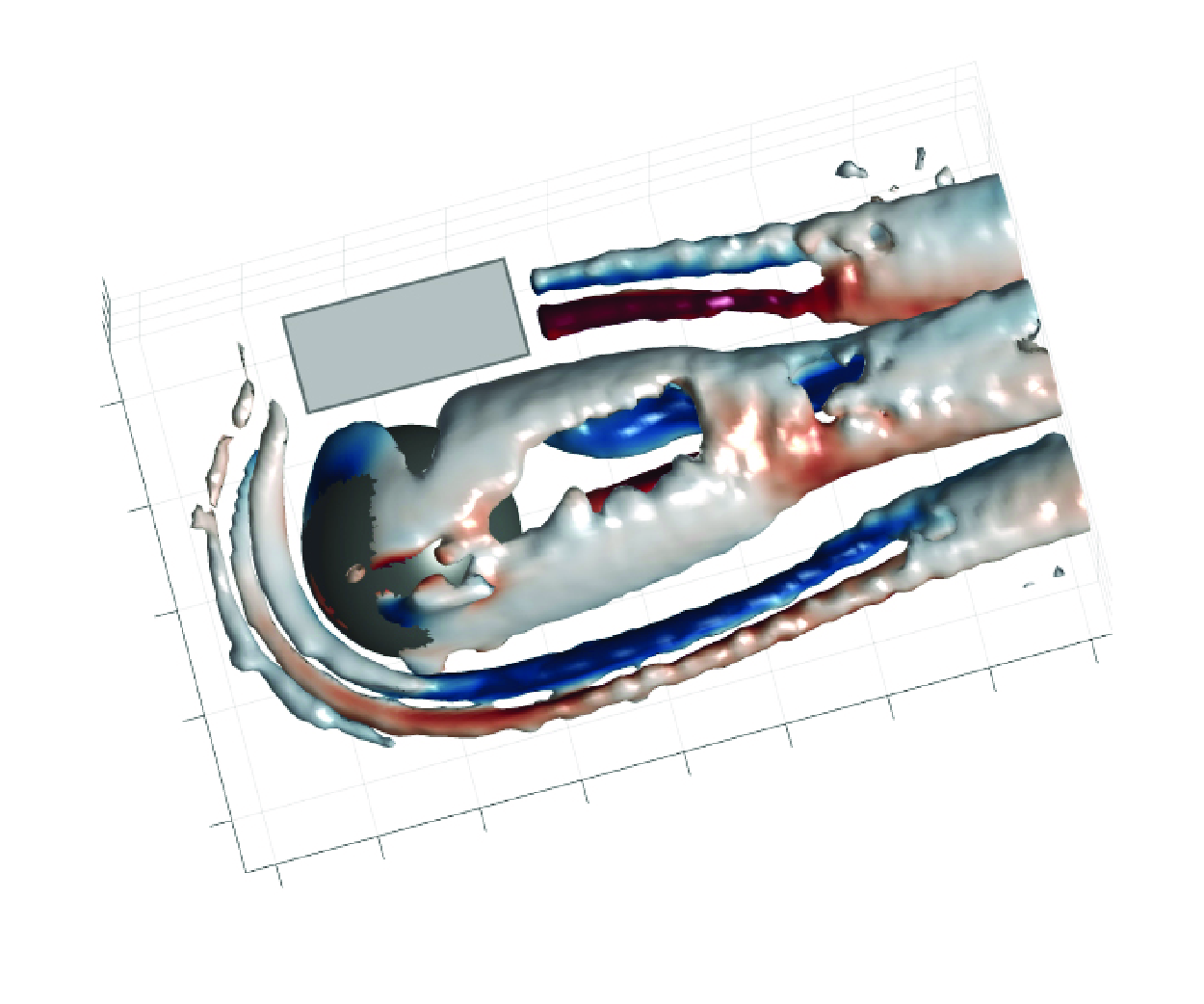
Time-averaged vortex structures around the hemisphere with the isosurface of
 $Q/(U_\infty /h)^2=0.03$
, which are coloured by the streamwise vorticity (
 $\overline {\omega _x}$
) contours. Partial missing within the
 $-0.5\lt x/h\lt 1.5$
,
 $y/h\gt 1$
range, indicated by the grey box, is due to model masking the laser sheet.

3. The flow structures
3.1. Time-averaged flow characteristics
The flow around a hemisphere submerged in a laminar boundary layer was found to have a notably complex 3-D separation flow. The salient features of the mean field around the hemisphere are summarised here as a basis for the analysis of interaction mechanisms between vortex structures. In this investigation, the
 $Q$
-criterion (Hunt et al. Reference Hunt, Wray and Moin1988; Jeong & Hussain Reference Jeong and Hussain1995) is employed to identify vortex structures, which is defined by the second invariant of the velocity gradient tensor. Figure 3 gives the isosurfaces of
 $Q/(U_\infty /h)^2=0.03$
and overlaid with time-averaged streamwise vorticity (
 $\overline {\omega _x}$
) contours, in which various vortex patterns are presented in the near wake. It should be noted that the similarity of the time-averaged flow field to Tu et al. (Reference Tu, Wang, Gao, She, Wang, Wang and Wei2023) confirms the accuracy of the current experiments.
A horseshoe vortex system formed upstream of the hemisphere is clearly observed in figure 3, which contains three separated vortex structures. In order to visualise this more intuitively, the structures upstream of the hemisphere are enlarged in figure 4(a) and are coloured using the spanwise vorticity contours. In addition, the vortex filaments of mean horseshoe vortices are extracted by the algorithm proposed by Wang et al. (Reference Wang, Shen, Mang, Gao, Wang and Wang2022) to identify the vortex cores. The basic idea of this algorithm is to represent the vortex field as a collection of discrete vortex atoms. By introducing a marching operation for the vortex atoms, their positions are iteratively updated, constantly marching towards the underlying vortex centrelines until these vortex atoms completely converge on curves. Thereafter, the vortex centrelines are obtained by tracking the converged vortex atoms. The state of the time-averaged HSV system is consistent with the ‘regime 2’ type referred to in Baker (Reference Baker1979), including a clockwise rotating main vortex, a small counter-rotating vortex, and another vortex rotating in the same direction as the main vortex upstream of the small counter-rotating vortex. It should be emphasised that this system is dynamic rather than steady. According to Baker (Reference Baker1979), the upstream HSV system exhibits complex oscillatory behaviours, including intermittent or random oscillations. However, only the time-averaged characteristics of the upstream HSV system are of interest here. As shown in figure 4(a), the primary HSV (HSV1) immediately adjacent to the model’s windward edge rolls up due to the obstruction of incoming flow by the hemisphere. It induces the reverse rotating secondary HSV (SHSV), and a new material surface similar to the hemisphere edge is then induced by the HSV1 and SHSV together. Another HSV rotating in the same direction as HSV1, denoted here as HSV2, is generated farther upstream under the blockage of this new material surface. Moreover, spatial locations of these three HSV structures are further emphasised based on figure 4(a). The SHSV is located between HSV1 and HSV2 in the streamwise direction, but its vertical position is lower than the other two vortices and closer to the wall.
(a) Time-averaged isosurface of
 $Q/ (U_\infty /h)^2=0.03$
and the centre-plane slice at
 $y/h=0$
coloured by the spanwise vorticity (
 $\overline {\omega _y}$
) contours. The black lines indicate the mean vortex filaments of horseshoe vortices. Magenta lines indicate the boundaries of vortices. (b) Streamwise vorticity
 $\overline {\omega _x}$
contours in the
 $x/h=-1.3,2,3.5,5$
planes overlapped by the velocity vectors.(c) Distribution of TKE in the central plane with streamlines superimposed on it.

As the horseshoe vortices extend downstream, they surround the bottom of the hemisphere, pulling out long streamwise vortex tubes symmetrically located on both sides of the recirculation zone. The reoriented streamwise extensions of HSV1 and SHSV possess opposite signs of streamwise vorticity, while the streamwise extensions of HSV2 are relatively weak in strength and do not persist for a long streamwise distance (
 $x/h\lt -0.5$
). For the sake of simplicity, the HSV structures upstream of the hemisphere and their corresponding streamwise extensions located downstream of the hemisphere are marked by the same symbols in this article. Figure 4(b) shows the distributions of time-averaged streamwise vorticity in the planes
 $x/h=-1.3,2,3.5,5$
. Downstream of the hemisphere, two pairs of counter-rotating streamwise vortices, consisting of HSV1 and SHSV, are symmetrically located away from the axial centre plane (
 $y/h=\pm 1\sim \pm 2$
, denoted in the black box in figure 4
b), as also shown in figure 3. These spanwise ranges roughly match the streamwise range of the HSV system upstream of the hemisphere in figure 4(a), confirming again that the upstream and downstream vortices describe the same entity. As the
 $\overline {\omega _x}$
contours in the spanwise cross-section indicated, streamwise extensions of HSVs all move away from the wall during convection downstream, while the SHSV lifts significantly faster. Behind the hemisphere, SHSV is located higher away from the wall than HSV1. Besides, a pair of counter-rotating mean streamwise vortices is also observed in the middle of the wake (
 $-1\lt y/h\lt 1$
). Their vortical characteristics are consistent with the definition of the base vortex (Wang & Zhou Reference Wang and Zhou2009), which is connected to the upwash flow. According to the theory of Hajimirzaie et al. (Reference Hajimirzaie, Wojcik and Buchholz2012) mentioned above, the shear layer from the hemisphere dominates the wake in this situation, and HVs tilt downstream. However, these base vortex structures may be artefacts of the averaging process since they are difficult to capture completely and stably in the instantaneous field. Herein, the base vortices are supposed to be the average result of the legs of hairpin vortices, which continuously shed behind the hemisphere. Figure 4(c) gives turbulent kinetic energy (TKE) contours in the central plane to examine the fluctuation intensities in the wake. The high turbulent intensity regions near the wall upstream of the hemisphere and higher than 1
 $h$
downstream of the recirculation zone correspond to the horseshoe vortices and heads of hairpin vortices, respectively, similar to the observation of Gao et al. (Reference Gao, Sun, Chen, Fan and Zhang2021). The high turbulence region near the wall in the wake may be associated with small-scale vortex structures near the wall, which is not the focus of this study.
(a) Plan view of the time-averaged streamwise velocity field in the plane
 $z/h=0.5$
. The vortical structures are visualised using the isosurface of
 $Q/(U_\infty /h)^2=0.03$
in transparent blue. (b) Conceptual sketches of the mean wake topology around the hemisphere. Grey and orange streaks indicate low- and high-speed regions, respectively.

Figure 5(a) depicts the distribution of time-averaged streamwise velocity in the
 $z/h=0.5$
plane. In the wake of the hemisphere, low- and high-streamwise-velocity regions occur alternately along the spanwise direction, and they are symmetrically distributed on both sides of the centre recirculation region. The counter-rotating streamwise vortices (consist of HSV1 and SHSV) induce upwash together between them, which pushes the low-momentum fluid near the wall upwards, giving rise to the low-speed region as shown in the simplified conceptual sketch in figure 5(b). Meanwhile, the average rotation direction of the hairpin vortex legs is opposite to that of HSV1 located on its ipsilateral outer side. They produce strong downwash motion and transport high-momentum fluid close to the wall, thus resulting in the two sidewise high-speed regions.
3.2. Developments of HV and SHV
The hairpin vortices and side hairpin vortices are the major characteristics in the wake of the hemisphere. It is therefore valuable to investigate in detail the evolution process of vortex structures, taking advantage of the highly accurate and 3-D flow field measurements.
Hairpin vortices originate from the recirculation region behind the hemisphere and are periodically shed downstream. This vortical structure occurs in the wake of many obstacles and plays significant roles in force generation and wake instability (Asgari et al. Reference Asgari, Saeedi and Etemadi2022; Vaid et al. Reference Vaid, Vadlamani, Malathi and Gupta2022). However, the evolution of its morphology still lacks investigation based on 3-D experimental results. The evolution of the HV’s shape as a function of the streamwise position of the HV head is illustrated in figure 6(a). Around
 $x/h=3$
, the head portion of a HV concentrates enough vorticity and then begins to tear a vortex tube from the strong shear layer downstream of the hemisphere. For
 $x/h\lt 4$
, the spanwise extent and vorticity of the vortex tube continuously increase, until a discrete hairpin-like vortex is discharged into the main flow. Subsequently, the head of the HV pulls out long streamwise vortex tubes as vortex legs from the recirculation region.
(a) Evolution path of the mean shape of HV. Vortices are presented by the isosurface of
 $Q/(U_\infty /h)^2=0.4$
with vortex filaments superimposed on them. The side projections of vortex filaments at
 $x/h=6$
is provided in the inset, where the definition of the angles between the leg and head parts of HV and the wall are defined here as
 $\theta _l$
and
 $\theta _h$
, respectively. (b) A representative instantaneous field of HV and the downwash motion described by the red isosurfaces correspond to
 $w'/U_\infty =-0.1$
.

In order to have better knowledge of the morphologic development along-streamwise of a whole HV, vortex centre filaments of the HV have been extracted by the algorithm proposed by Wang et al. (Reference Wang, Shen, Mang, Gao, Wang and Wang2022) (described above). Figure 6(a) provides the vortex centrelines superimposed on the corresponding vortex structures at each specific streamwise position, and the side projections of these vortex centrelines are analysed to display more details of the HV. The portions of leg and head of projections are focused on separately, and the angles between these two parts and the wall are defined as
 $\theta _l$
and
 $\theta _h$
, respectively, as denoted in the inset in figure 6(a). Variations of the
 $\theta _l$
and
 $\theta _h$
are presented in figure 7(a). It is interesting that the morphological evolution of HV can be divided into two stages according to the characteristics of the angles of the vortex head and legs. The angle between the head portion of HV and the wall first decreases until
 $x/h=5.5$
, and then it slightly increases. This suggests that during the formation of HV, it keeps tilting downstream, thus splitting from the shear layer. This downstream inclination also implies that the shear layer, rather than Biot–Savart self-induction, dominates the formation of HV. After
 $x/h=5.5$
, the influence of the shear layer is weakened, allowing HV to be more affected by the Biot–Savart self-induction. At this stage, HV sheds downstream independently while the vortex head lifts away from the wall, leading to a small increase of
 $\theta _h$
.
(a) Evolution of the angles between the leg and head portions of HV and the wall, indicated by the black and dotted lines, respectively. (b) Conditional-averaged of the convecting streamwise velocity (
 $u_{conv}$
) of the HV head and time-averaged streamwise velocity (
 $\overline {u}$
) at the mean trajectory of it, indicated by the black and magenta lines, respectively.

Furthermore, once a HV pulls out vortex legs from the recirculation region, its leg portions are inclined towards the wall (
 $\theta _l\lt 0$
) until its head reaches roughly
 $x/h=5.5$
. Afterwards, the
 $\theta _l$
continually increases and the legs of HV tilt away from the wall (
 $\theta _l\gt 0$
), as indicated by the dotted line in figure 7(a). The variation of the convective velocity of the HV head along the streamwise direction is further given in figure 7(b) to elaborate on the reason for the reverse tilt of the HV legs. As shown by the black line in figure 7(b), while the hairpin vortices convect downstream, the convective velocity increases rapidly until it tends to be constant after
 $x/h=5.5$
. Since the hairpin vortex sheds at a certain frequency (detailed below), the flow distance between two neighbouring vortex structures is likewise increasing. Each hairpin vortex head induces a strong downwash (indicated by the red isosurface of
 $w'/U_\infty =-0.1$
) on its downstream side, as illustrated in figure 6(b), transporting high momentum free stream towards the wall. When a HV is very close to the newborn HV upstream of it, its leg-head junction would be squeezed by the downwash event induced by the newborn HV. Therefore, there is a phenomenon of the hairpin vortex legs tilting towards the wall (
 $\theta _l\lt 0$
). However, the distance between the two adjacent HVs increases as they convect downstream. Consequently, the location of the former generated HV being squeezed by the downwash event continues to move upstream. Thus,
 $\theta _l$
continually increases until the distance is far enough, after
 $x/h=5.5$
that the downwash of the later HV can only affect the end of the leg portion of the former HV, at which situation the
 $\theta _l\gt 0$
.
In short, the hairpin vortex shedding process was categorised into two stages based on its morphology: the formation stage before
 $x/h=5.5$
, and the convection stage downstream. The major distinction between them is the inclination direction of the HV legs. During the convection stage of hairpin vortex, all its parameters tend to be stabilised. Each hairpin vortex evolves downstream essentially individually.
Since HVs originate from the recirculation region behind the hemisphere, low-speed fluids are carried inside their vortex tube. The head portions of HV correspond to the localised region of low streamwise velocity. In addition, in the interval of hairpin vortex periodical shedding, the high-speed fluid will be induced by HV heads to enter the near wall region. Therefore, the time-averaged streamwise velocity at the mean trajectory of the HVs’ heads are bigger than the conditional-averaged streamwise velocity of them along with the streamwise locations, as shown in figure 7(b). In other words, velocity defects in a hemispherical wake are mainly caused by the shedding of hairpin vortices.
Similarly, the morphological evolution of side hairpin vortices has also been investigated. The SHV originates from the counter-rotating streamwise vortex pair consisting of HSV1 and SHSV. These two vortical structures induce upwash motions between them, ejecting the low-speed fluid away from the wall. It interacts with the external high-speed flow to form a strong shear layer and leads further to the roll-up of the arch-shape vortex tube. This vortex tube straddles the pair of HSV streamwise extensions, as shown in figure 8(a). As more vorticity and mass are dragged out from the streamwise extensions of HSV by the vortex tube during convecting downstream, it becomes a fully developed SHV. Back to figure 4(b), HSV1 is significantly stronger than SHSV at
 $x/h=2$
. However, SHSV becomes progressively stronger, and HSV1 becomes weaker as the streamwise position increases. Combined with figure 8(a), SHV acts as a bridge connecting the pair of streamwise extensions of HSV, continuously transporting vorticity from HSV1 to SHSV.
Since the scale and vertical extent of SHV are relatively small compared with HV, and the distinctions between its vortex legs and head are not obvious, the present work considers SHV as a whole for research. Figure 8(c) gives the variation of the angle between SHV and the wall. It can be seen that the SHV keeps tilting towards the wall until
 $x/h\gt 5$
almost constant. Similar to HV, the shedding process of SHV is also divided into two stages. The formation stage is in the range of
 $x/h\lt 5$
, where the vortex tube continually gains vorticity from HSVs. At approximately
 $x/h=5$
, SHV is disconnected from the streamwise extensions of HSV and convects individually as shown in figure 8(a,b). Thus, after
 $x/h=5$
is the convection stage. It is important to note that the SHSV is always in a higher vertical position than HSV1 during the generation of SHV. This results in the inner vortex legs of the SHV being much stronger than the outer legs, as clearly indicated in figure 8(b). In fact, SHVs are not with standard symmetric arch shapes as mentioned previously (Ye et al. Reference Ye, Schrijer and Scarano2016), but rather exhibit tilted arch shapes shifted to the centre.
Panels (a) and (b) are the axonometric and side view of the representative instantaneous field of the side hairpin vortex. Isosurface of
 $Q/(U_\infty /h)^2=0.1$
is coloured by streamwise vorticity. (c) Evolution of the angle between SHV and the wall.

4. Vortex dynamics in the wake
In this section, the vortex dynamics of the vortical structures in the near wake of a hemisphere are explored in an attempt to elucidate the interaction between HV and SHV and their common effects on the hemisphere wake.
4.1. The POD coefficients and spectrum analysis
The POD analysis was performed on the whole dataset within the wake region (
 $x/h=2{-}6.5,y/h=-2.5{-}2.5,z/h=0{-}2$
) for all three velocity components. Before the POD calculation, the mean velocity is subtracted from the dataset. The energy distribution (
 $\lambda _n/\sum \lambda _n$
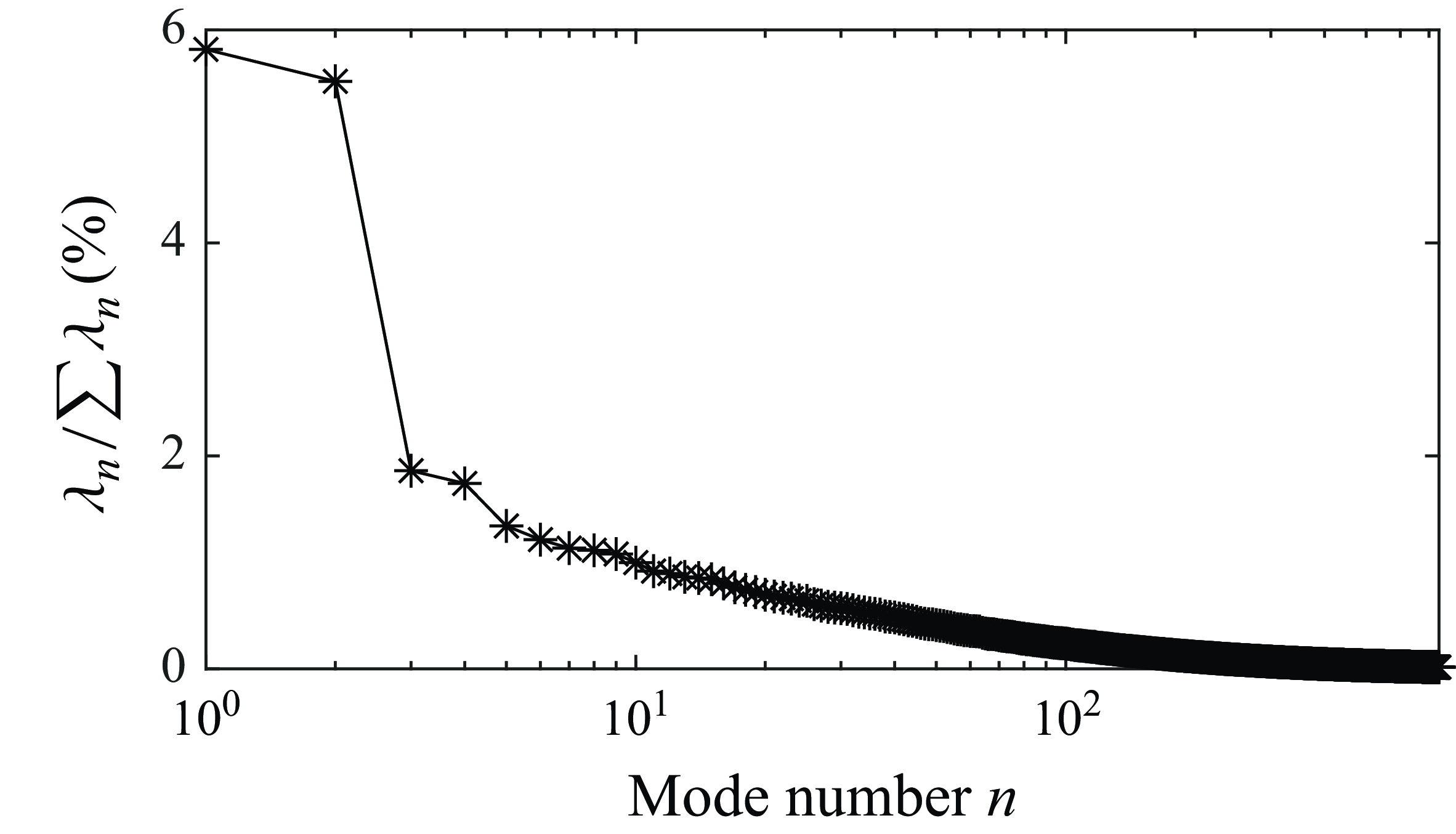
) for all POD modes is given in figure 9. It is indicated that the energies contained by the first two POD modes are very close and significantly higher than those of the other modes. This suggests that the first two modes dominate the hemispherical wake. Despite the low absolute energy content of the first mode, the key point in the POD analysis is its relative energy predominance. The first two modes occupied approximately three times the energy of mode 3 and mode 4, and many multiples of the other modes. Therefore, the low energy content of the first modes does not impact the determination of the periodic feature, as shown by the results below.
Relative energy distributions of the different POD modes.

(a) The PSD of modes 1 (black line) and 2 (magenta line). (b) Dimensionless
 $Q$
isosurfaces of the first two POD modes with different colours to distinguish different modes. The red and blue isosurfaces mark mode 1 and mode 2, respectively.

In order to investigate the periodic features of the dominant vortical structures, the power spectral density (PSD) of POD time coefficients of the first two modes is presented in figure 10(a). As shown by the spectrum analysis, mode 1 and mode 2 present clearly periodic characteristics and share the same peak at Strouhal number
 $St=fh/U_\infty =0.36$
. Figure 10(b) further presents the spatial characteristics of the first two modes with dimensionless
 $Q$
isosurfaces to clarify the flow pattern. Obviously, mode 1 and mode 2 are a pair of conjugated modes with a phase difference that govern the periodical shedding of hairpin vortices in the middle of the wake. Spectrum analysis on the velocity fluctuations
 $u'$
and
 $w'$
is executed at the head portions of hairpin vortices with different streamwise locations (
 $x/h=2.5{-}6,y/h=0,z/h=1.1$
) to validate the vortex-shedding frequency again, as shown in figure 11(a). Along the streamwise direction, both
 $u'$
and
 $w'$
have a dominant frequency
 $St_1=0.36$
, and the corresponding amplitudes increase as the HVs convey downstream. This is consistent with the frequency peak of POD modes 1 and 2, which reveals that the generation of HV is dominated by POD modes 1 and 2. Since HV is the most important vortical characteristic in the hemisphere wake, naturally, the dominant frequency of the shedding of HV is denoted here as
 $St_1$
, and the first and second POD modes are referred to as the hairpin vortex shedding modes (HV-S).
The PSD of streamwise (
 $u$
) and vertical (
 $w$
) velocity fluctuations at the head portions of (a) HVs, and (b) SHVs with different streamwise locations. Black and magenta lines indicate
 $u'$
and
 $w'$
, respectively.

In addition, a weaker low-frequency peak
 $St=0.18$
gradually appears in the hairpin vortex head region after approximately
 $x/h=3.5$
, as shown in figure 11(a). It is almost half of the base frequency
 $St_1$
of HV shedding, so we denote it as half-frequency
 $St_{1/2}$
. In the present work, the half-frequency
 $St_{1/2}$
corresponds to a new topology: an asymmetric arranged vortex pattern, and further discussion will be provided in § 4.2.
Figure 11(b) presents the power spectra of the velocity fluctuations at the head regions of SHV (
 $x/h=2.5{-}6,y/h=-1.35,z/h=0.85$
). Unlike HV, the dominant frequency of the SHV region is
 $St=0.57$
. It is almost 1.5 times the base frequency
 $St_1$
of the HV shedding, so we denote the dominant frequency of the SHV shedding as
 $St_{3/2}$
. The difference between SHV and HV shedding primary frequencies is due to the fact that their shedding processes are determined by different POD modes. It is found in figure 12(a) that the identical peak at
 $St_{3/2}=0.57$
in the power spectra of the time coefficients of seventh and eighth POD modes as the frequency of the SHV shedding. Moreover, the spatial distributions of the seventh and eighth modes (figure 12
b) indicate that these two modes compose another conjugated pair with a phase difference, which is characterised by the alternating vortex structures along the streamwise direction. This suggests that the seventh and eighth conjugate POD modes correspond to the shedding and convection processes of the SHV, thus denoted as side hairpin vortex shedding (SHV-S) modes. It should be emphasised that the SHV-S and HV-S modes are spatially independent. The HV-S mode is located in the centre of the hemisphere wake, while the SHV-S mode is symmetrically distributed on the outside of the HV-S mode. Because of this, the two modes are actually the most energetic at their corresponding spatial locations, respectively. Hence, the HV-S and SHV-S modes govern the two primary vortex features in the near wake: the shedding of HV and SHV, respectively. Besides, the third to sixth modes are essentially in the same spatial region as the HV-S modes, with weak interactions with the SHV-S modes. They have lower energy contents than the HV-S modes and thus are the high-order modes that effect the evolution of vortex structures rather than being dominant. Herein, this subsection focuses on the dominant modes of the two characteristic vortex structures, ignoring the influence of other higher-order modes.
(a) The PSD of modes 7 (black line) and 8 (magenta line). (b) Dimensionless
 $Q$
isosurfaces of the seventh and eighth POD modes with different colours to distinguish different modes. The magenta and cyan isosurfaces mark mode 7 and mode 8, respectively.

4.2. Mechanism of asymmetric shedding
In addition to the canonical shedding pattern exhibiting discrete HV with spanwise symmetrical distribution, a new pattern exhibiting asymmetry in the shedding of hairpin structures is novel in the current study. The analogous phenomenon has been reported in past literature: the wake of the wall-mounted prism (Goswami & Hemmati Reference Goswami and Hemmati2022), and hemispherical wakes with higher Reynolds numbers (Fu et al. Reference Fu, Cheng, Lo and Cheng2015; Cao & Tamura Reference Cao and Tamura2020; Li et al. Reference Li, Qiu, Shao, Liu, Fu, Tao and Liu2022). In these studies, asymmetric wakes usually occur in a particular range of flow parameters, and the coexistence of asymmetric and symmetric patterns is less reported. Thus, to the authors’ knowledge, this is the first time that the coexistence of two shedding patterns has been observed in the hemispherical wake at low Reynolds numbers. The following paragraphs provide a detailed analysis of the mechanism of asymmetric modes.
(a) The PSD of modes 3 (black line) and 4 (magenta line). Panels (b) and (c) are the dimensionless
 $u'$
isosurfaces, and the
 $u'$
contours in the
 $z/h=0.5$
planes of the third and first POD modes, respectively.

Figure 13(a) illustrates the power spectra of the time coefficients of POD modes 3 and 4, which share the identical peak at Strouhal number
 $St_{1/2}$
. It is consistent with the half-frequency
 $St_{1/2}=0.18$
in the spectra of flow velocity fluctuations of HV, as shown in figure 11. This suggests that the half-frequency feature in the hemisphere wake field is supposed to be governed by the conjugate third and fourth POD modes. Unlike the typical hairpin vortex shedding pattern with spanwise symmetry controlled by HV-S modes in figure 13(c), a clear spanwise asymmetric pattern can be observed in the spatial distributions of the third mode (figure 13
b), which may result in the asymmetric shedding behaviours of HVs. This arrangement is in agreement with the typical arrangement observed in the sinuous instability mode (Vaid et al. Reference Vaid, Vadlamani, Malathi and Gupta2022). Due to this mode making the hemispherical wake oscillate laterally alternately, it is referred to as the asymmetric shedding mode (A-S). As shown in figure 13(b), the A-S pattern occurs more in the HV region and has less effect on the SHVs. Consequently, the amplitude of the frequency
 $St_{1/2}$
of asymmetric modes in the fluctuation velocity spectrum corresponding to the HV is larger than in the SHV, which is consistent with the observations in figure 11.
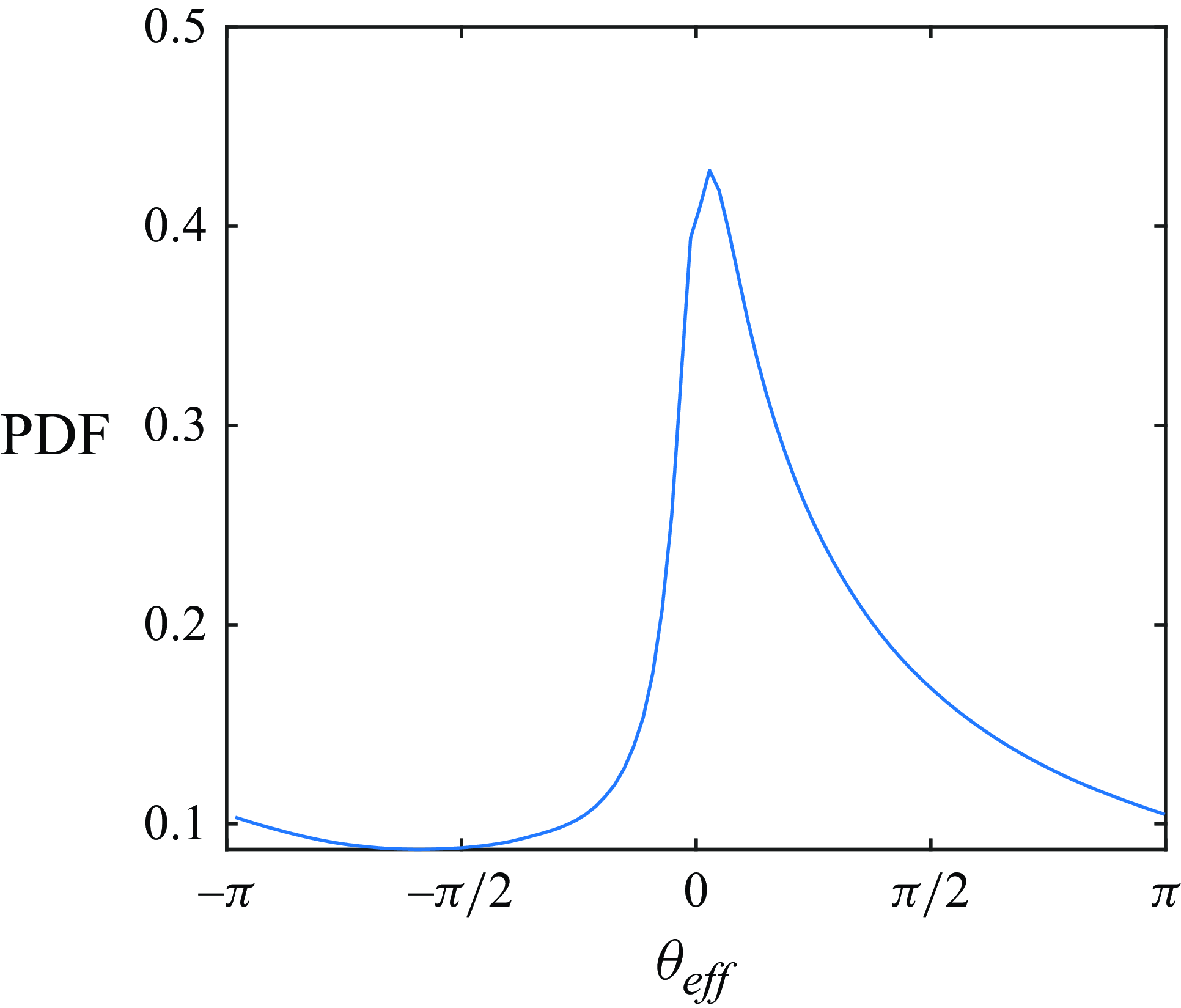
The probability density function (PDF) of the effective phase angle
 $\theta _{\textit{eff}}$
.

Furthermore, the interaction between the HV-S and A-S modes and their contributions to the dynamics in the wake are explored. Recalling the above results, the dominant frequency of the A-S mode is almost half of the HV-S mode. Consequently, the HV-S mode can be considered the fundamental wave, and the A-S mode its subharmonic. According to Arbey & Williams (Reference Arbey and Williams1984) and Gordeyev & Thomas (Reference Gordeyev and Thomas1999), the interaction between the fundamental and subharmonic waves depends on their effective phase angle. Therefore, the phase angles of HV-S and A-S modes are obtained, respectively, by (Liu et al. Reference Liu, Wang, Zhu and Pan2024)
 \begin{align}& {\theta _{HV-S}=\arctan \left(\frac {a_1\sqrt {2\lambda _2}}{a_2\sqrt {2\lambda _1}}\right )}, \\[-12pt] \nonumber \end{align}
 \begin{align}&\,\, {\theta _{A-S}=\arctan \left(\frac {a_3\sqrt {2\lambda _4}}{a_4\sqrt {2\lambda _3}}\right )}. \end{align}
Then the effective phase angle is defined as
 \begin{equation} {\theta _{eff}=\theta _{HV-S}-2\theta _{A-S}}. \end{equation}
Figure 14 gives the PDF of the effective phase angle
 $\theta _{eff}$
. It can be seen that the probability is highest when the
 $\theta _{eff}$
is approximately 0, which indicates that these two modes are consistently resonant in the hemisphere wake.
Additionally, it is known that the characteristics of the instantaneous flow field have closely corresponding connections with the amplitude of the time coefficients (Wang et al. Reference Wang, Cao and Zhou2014), and thus the POD coefficients of the two modes characterise their influence on the shedding behaviour of HVs. Specifically, when the amplitude of the time coefficient is less than 10
 $\%$
of its maximum value, the corresponding POD mode is considered to have a relatively weak influence on the flow field. Therefore, the symmetric pattern is deemed to dominate the middle of the hemispherical wake when the amplitude of the time coefficient of the first mode, namely
 $\left | a_1 \right |$
, reaches its local maximum and the amplitude of the coefficient of the third mode, namely
 $\left | a_3 \right |$
, is lower than the threshold. The hairpin vortices in the resultant conditionally averaged flow field exhibits a typical symmetric shedding pattern as shown in figure 15(a). Conversely, when the
 $\left | a_3 \right |$
reaches its local maximum and the
 $\left | a_1 \right |$
is below the threshold, hairpin vortices manifest very pronounced asymmetric behaviours, as shown in figure 15(b,c). However, the difference in the HV deflection direction in figure 15(b,c) arises from the fact that they present the conditional averaged flow fields corresponding to the
 $\left | a_3 \right |$
reaching its positive and negative local maximums, respectively, under the above asymmetric shedding conditions. Consequently, the sign of
 $a_3$
determines the deflection direction during asymmetric shedding of HVs. Since the HV-S mode contains more energy than the A-S mode, the middle of the hemispherical wake is more controlled by the HV-S mode. The presence of the A-S mode would cause the hairpin vortex shedding patterns to transfer from symmetric to asymmetric. To be emphasised, the transition between symmetric and asymmetric shedding patterns of HV is not abrupt. Typical symmetric shedding patterns would gradually distort and transform to the asymmetric patterns, and vice versa. In conclusion, the shedding behaviour of the hairpin vortices at the current Reynolds number is a result of the combined expression of these two modes.
Top view of the conditional averaged flow fields with the isosurface of
 $Q/(U_\infty /h)^2=0.36$
for three cases, namely (a) symmetric and (b, c) asymmetric with different deflection directions.

It is surprising that the SHV structures are not strictly symmetric along the spanwise direction in the present work. Since the SHV-S mode mainly governs the shedding pattern of SHVs, our attention is again devoted to their spatial distribution to validate this fact. As shown in figure 12(b), the patterns of SHVs on both sides of the wake indeed exhibit spanwise asymmetry. To determine whether the asymmetry of SHVs is related to the characteristics of the streamwise extensions of HSV, the correlation coefficients are calculated between the streamwise velocity fluctuations at two spanwise symmetric locations, obtained from the region of maximum velocity fluctuations within the SHV region, as shown in figure 16. The coefficient is defined as
 \begin{equation} R=\frac {\left\langle u'(t)|_{x_0,y_1,z_0} u'(t)|_{x_0,y_2,z_0}\right\rangle _t}{\sigma \left(u'(t)|_{x_0,y_1,z_0}\right)\sigma \left(u'(t)|_{x_0,y_2,z_0}\right)}, \end{equation}
where
 $\langle \cdot \rangle _t$
is taking the average along time and
 $\sigma$
is the standard deviation. As expected, the high correlation has been observed between the structures on both sides of the hemisphere wake. Interestingly, the phase difference between the structures on both sides remains constant along the streamwise direction, even where the SHV has not yet rolled up. Here the phase difference is defined as the horizontal coordinate where the correlation coefficient reaches its peak as indicated by the red dot in figure 16, which is
 $\Delta t/T_{SHV}=0.17$
(
 $T_{SHV}$
represents the period of SHV shedding), approximately equal to
 $\pi / 3$
. This suggests that spanwise asymmetric perturbations are consistently existing in the symmetric regions on both sides of the hemisphere. These perturbations are transported downstream along the streamwise extensions of HSVs and lead to their asymmetric oscillations. Simultaneously, SHVs are always formed and shed asymmetrically, irrespective of the shedding pattern of HVs in the middle of the wake.
Temporal cross-correlation of the streamwise velocity fluctuations at two spanwise symmetric locations in the region of maximum velocity fluctuations within the regions of SHV at different streamwise locations.

Such a vortical shedding pattern is different from our previous observations with lower Reynolds numbers (Liu et al. Reference Liu, Wang, Zhu and Pan2024). At lower Reynolds numbers
 ${\textit {Re}}_h=780$
, hairpin vortices always shed periodically in a symmetric pattern behind the hemisphere, while the streamwise extensions of HSV on both sides also oscillate symmetrically about the centre plane. The SHV structures were not identified due to limitations in experimental conditions, but since they were induced by the streamwise extensions of HSV, it is reasonable to speculate that SHV should also be shed symmetrically. As the Reynolds number increases, the complexity of the hemispherical wake increases, and the shedding patterns also vary. According to the above facts, the shedding pattern of SHV at the current Reynolds number has completely transformed into an asymmetric pattern attributed to the asymmetric oscillation and breakdown of the streamwise extensions of HSV, which is totally different from our former study. However, the symmetric and asymmetric patterns still coexist during the shedding process of HV currently. Again, it should be emphasised that the asymmetric behaviours of SHV are not affected by the variation of HV patterns. This phenomenon suggests that the formation of asymmetric shedding pattern of HV should be attributed to asymmetric perturbations in the HSVs, rather than that the asymmetric behaviours of HSV are caused by HV. Specifically, the asymmetricity of the streamwise extensions of HSV, which simultaneously induces the asymmetric shedding of the SHV, transports instability to the middle of the wake, causing the shedding pattern of HV to begin to transfer from symmetric to asymmetric. Afterwards, with the further increase of Reynolds number, asymmetricities in the streamwise extensions of HSV enhance and dominate the hemispherical wake field, which completely transfers into the asymmetric shedding pattern, as Fu et al. (Reference Fu, Cheng, Lo and Cheng2015), Cao & Tamura (Reference Cao and Tamura2020) and Li et al. (Reference Li, Qiu, Shao, Liu, Fu, Tao and Liu2022) described.
5. Conclusion
The present study investigates the 3-D flow structures over a 10 mm height hemisphere at Reynolds number
 ${\textit {Re}}_h=1530$
using TPIV. The hemisphere is completely immersed in a laminar boundary layer of
 $\delta /h=1.12$
. The novelty of this study lies in revealing the mechanism of the asymmetric shedding pattern in the near wake, which is the first time it has been found at such a low Reynolds number. Meanwhile, the evolution characteristics of typical coherent structures around a hemisphere are detailed discussed.
The HV and SHV structures are formed periodically in the middle and both sides of the wake behind the hemisphere, respectively. Their morphological evolution processes have been revealed. The fundamental evolution routine of HV can be divided into formation and convection stages according to the characteristics of the angles of its head and leg portions. During the formation stage, the head portion of HV is tilted downstream, indicating that the shear layer dominates the HV formation. Meanwhile, the HV’s leg portion inclines towards the wall, which is attributed to the downwash induced by the newborn HV upstream of it at a sufficiently close distance. On the contrary, the head of HV is slightly inclined upstream while the legs tilt away from the wall in the convection stage. This is because once a HV begins to shed downstream individually, the effect of pushing it upstream by Biot–Savart self-induction gradually manifests, as the effect of the shear layer diminishes. At the same time, the distance between two consecutive hairpin vortices is large enough that the downwash of the latter HV can only affect the end of the leg of the former. Similarly, the morphological evolution of SHV is also categorised into two stages. In the formation stage, SHV continually gains vorticity from the streamwise extensions of HSV until it is disconnected from HSVs and convects individually, beginning the convection stage.
The vortex dynamics governing the two typical structures are further revealed by POD analysis. The shedding processes of HV and SHV are dominated by two different POD modes: the HV-S mode and SHV-S mode, respectively, with correspondingly different characteristic frequencies. In addition to the primary spanwise symmetric shedding pattern of HV, an asymmetric shedding pattern is also observed in the instantaneous flow field at the current Reynolds number. This asymmetric behaviour is controlled by the A-S POD mode, whose dominant frequency is exactly half of that of the HV-S mode. At the current Reynolds number, the shedding behaviour of the hairpin vortices is a result of the combined expression of the HV-S and A-S modes, and the sign of the time coefficient corresponding to the A-S mode determines the direction of the HV deflection.
Furthermore, SHVs on both sides of the wake are throughout formed and shed alternately, and the corresponding streamwise extensions of HSV also oscillate asymmetrically. It is unlike the spanwise symmetrical oscillation of the streamwise extensions of HSV observed in our previous study (Liu et al. Reference Liu, Wang, Zhu and Pan2024) at a lower Reynold number. The SHV shedding mode at the current Reynolds number has completely changed to an asymmetric mode, while symmetric and asymmetric modes still coexist during HV shedding. It is reasonable to speculate that when the Reynolds number is higher, the asymmetricities in the streamwise extensions of HSV further enhance and dominate the hemispherical wake, which completely transfers into the asymmetric shedding pattern. Of course, this process needs to be confirmed by subsequent studies. In short, the present results fill gaps in interaction between HSV, HV and SHV, and promote the further application of wall-mounted obstacles in flow control.
Funding.
This work was supported by the National Natural Science Foundation of China (no. 11721202).
Declaration of interests.
The authors report no conflict of interest.
Appendix A. A portfolio of POD modes
The PSD of time coefficients of the first 12 POD modes.

Spatial distributions of the first 12 POD modes with streamwise velocity fluctuation
 $u'$
contours.

In the current work, POD analysis was conducted to investigate the dynamics and evolution of vortical structures in the hemisphere wake. In this appendix, we provide the PSD of the time coefficients and the spatial distributions for the first 12 POD modes as shown in figure 17 and figure 18, respectively. Since the higher-order modes (beyond the 12th) contain considerably lower energy, their influences on large scale structures are negligible and thus omitted. It is seen in figure 17 that the first 10 POD modes occur in pairs, with each pair possessing the same dominant frequency. Specifically, the dominant frequency of the first two modes is
 $St_1=0.36$
, the third to sixth modes share the same peak frequency at
 $St_{1/2}=0.18$
, and the seventh to 10th modes share the same peak frequency at
 $St_{3/2}=0.57$
. It should be noted that no sum of these three frequencies is observed in the first 12 modes, which may indicate that the nonlinear interaction between the three frequencies is quite weak. Interestingly, although the dominant frequencies of the third to sixth POD modes are all
 $St_{1/2}=0.18$
, their spatial distributions (figure 18
c–f) suggest that they correspond to two different flow mechanisms, respectively. The fifth and sixth modes are unrelated to alternating asymmetric shedding governed by the A-S mode (the third and fourth modes) but may describe other instability mechanisms of the hairpin vortex. Furthermore, the seventh to 10th POD modes constitute two separate sets of mode pairs, although they both correspond to SHV shedding and convection. For brevity, only the seventh and eighth modes are discussed in the main text.
Appendix B. Further discussion of
 $\boldsymbol{St}_{\boldsymbol{1/2}}$

This appendix provides further discussion for the physical interpretation of the lowest frequency
 $St_{1/2}$
in the hemisphere wake. The difference between the original flow fields
 $U(x,y,z,t)$
and their mirrored counterparts
 $U_{mirror} (x,-y,z,t)$
symmetric along the
 $y=0$
plane is calculated, referred to as
 $\Delta U(x,y,z,t)$
. Naturally, the spatially averaged value of
 $\Delta U(x,y,z,t)$
, denoted as
 $\overline {\Delta U}(t)$
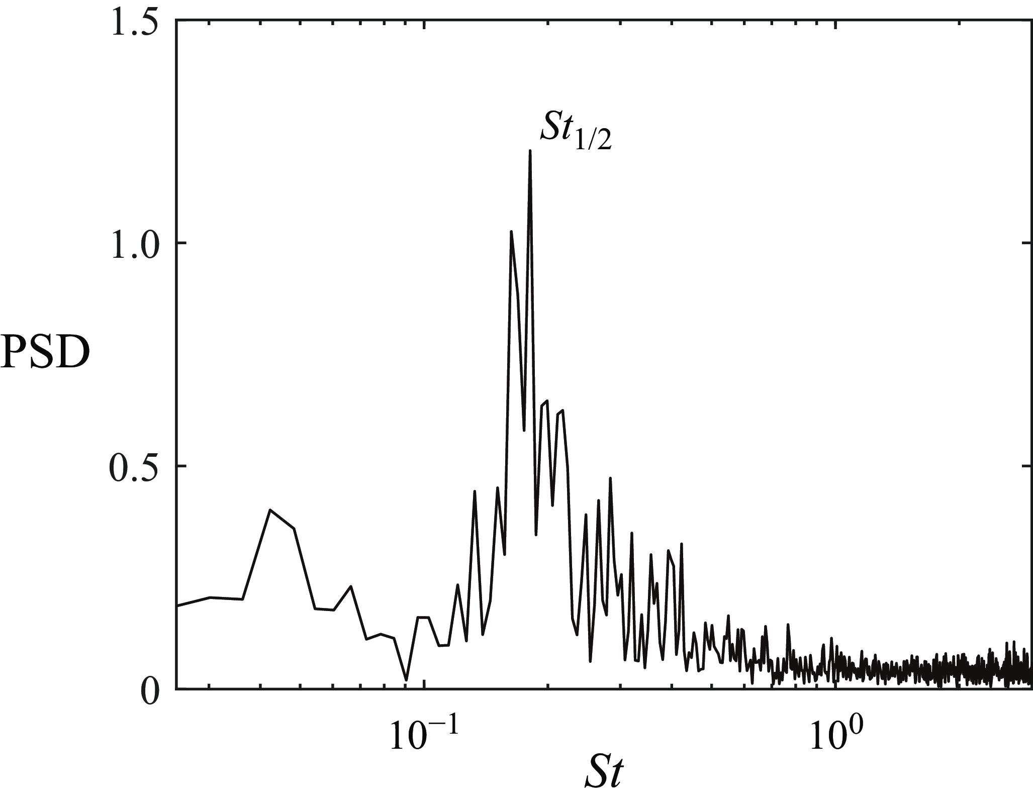
, varies with time. Its magnitude indicates the degree of asymmetry of the wake flow. The spectrum of
 $\overline {\Delta U}(t)$
is given in figure 19, which possesses the same dominant frequency of
 $St_{1/2}=0.18$
. Once again, it confirms that the lowest frequency
 $St_{1/2}$
corresponds to the asymmetry in the wake of the hemisphere.
The PSD of
 $\overline {\Delta U}(t)$
.