1. Introduction
The mechanisms underlying pattern formation in suspensions of swimming micro-organisms have been the continued subject of fluid dynamical study since at least the mid-1980s, when Kessler (Reference Kessler1985, Reference Kessler1986) published his observations of collective behaviour of upswimming denser-than-water biflagellate algal cells of the genera Chlamydomonas and Dunaliella. The cells swim upwards in still fluid, on average, because they are bottom-heavy; the Reynolds number of the relative motion is invariably very small. When the ambient fluid is in motion, the cells experience a viscous torque proportional to the local vorticity (and another, proportional to the strain rate, for non-spherical cells); their orientation is then determined by a balance between viscous and gravitational torques, in a process known as gyrotaxis (Kessler Reference Kessler1985). Pattern-forming instabilities (bioconvection) can arise either from the unstable density stratification generated by upswimming near the upper surface of a chamber (Platt Reference Platt1961) or from the spontaneous gyrotactic generation of focused plumes in a deep chamber, far from the boundaries (Kessler Reference Kessler1986), or from a combination of the two.
Much modelling of bioconvection in suspensions of gyrotactic cells has been based on linear instability theory applied to a dilute suspension. Here, ‘dilute’ means that the cell number density
 $n$
(and hence volume fraction) is assumed to be sufficiently small that hydrodynamic interactions between cells are negligible, although of course it must be large enough for gravity-driven bulk motions to develop from perturbations to
 $n$
. The equation of conservation of cells in such a suspension may be taken to be
 $$\begin{eqnarray}\frac{\partial n}{\partial t}=-\boldsymbol{{\rm\nabla}}\boldsymbol{\cdot }[n(\boldsymbol{u}+\boldsymbol{V}_{C}+\boldsymbol{V}_{G})-(D\boldsymbol{\cdot }\boldsymbol{{\rm\nabla}}n)],\end{eqnarray}$$
where
 $\boldsymbol{u}(\boldsymbol{x},t)$
is the fluid velocity field,
 $\boldsymbol{V}_{C}(\boldsymbol{x},t)$
is the average cell swimming velocity,
 $\boldsymbol{V}_{G}(\boldsymbol{x},\!t)$
is the gravitational sedimentation velocity and the last term represents randomness in cell swimming by means of a translational diffusivity tensor
 $D(\boldsymbol{x},t)$
. The earliest models assumed that all cells swim either vertically upwards (Childress, Levandowsky & Spiegel Reference Childress, Levandowsky and Spiegel1975) or in a direction determined by the torque balance on each of the supposedly identical cells (Pedley, Hill & Kessler Reference Pedley, Hill and Kessler1988; Hill, Pedley & Kessler Reference Hill, Pedley and Kessler1989). In both cases, this is inconsistent with the observations that each cell performs a random walk and that the cells are not all identical, factors assumed to be satisfactorily accounted for by the diffusivity
 $D$
. A more rational model was introduced by Pedley & Kessler (Reference Pedley and Kessler1990), who proposed that the randomness should be represented by a rotational diffusivity
 $D_{R}$
, so that the cell orientation
 $\boldsymbol{p}$
(a unit vector) would be a random variable, whose probability density function
 $f(\,\boldsymbol{p})$
satisfies the quasi-steady Fokker–Planck equation, a partial differential equation in
 $\boldsymbol{p}$
-space:
 $$\begin{eqnarray}\boldsymbol{{\rm\nabla}}_{p}\boldsymbol{\cdot }(\,\dot{\boldsymbol{p}}f)=\boldsymbol{{\rm\nabla}}_{p}\boldsymbol{\cdot }(D_{R}\boldsymbol{\cdot }\boldsymbol{{\rm\nabla}}_{p}\,f),\end{eqnarray}$$
where
 $\dot{\boldsymbol{p}}$
is the rate of change of
 $\boldsymbol{p}$
driven by the gravity–viscous torque balance. Quasi-steadiness relies on the assumption that the time scale for the cell orientation distribution to respond to changes in the local vorticity, for example, and hence changes in
 $\dot{\boldsymbol{p}}$
, is very much shorter than the time scale over which those changes take place. In the absence of other information, Pedley & Kessler (Reference Pedley and Kessler1990) also assumed that
 $D_{R}$
is constant and isotropic of magnitude
 $D_{R}$
.
The gyrotactic torque balance, based on Stokes flow around a small spheroid, gives
 $$\begin{eqnarray}\dot{\boldsymbol{p}}=B^{-1}[\boldsymbol{k}-(\boldsymbol{k}\boldsymbol{\cdot }\boldsymbol{p})\boldsymbol{p}]+{\textstyle \frac{1}{2}}\hat{{\bf\omega}}\wedge \boldsymbol{p}+{\it\alpha}_{0}\,\boldsymbol{p}\boldsymbol{\cdot }\hat{\unicode[STIX]{x1D640}}\boldsymbol{\cdot }(\unicode[STIX]{x1D644}-\boldsymbol{pp}),\end{eqnarray}$$
where
 $k$
is a unit vector directed vertically upwards,
 $\hat{{\bf\omega}}$
is the vorticity,
 $\hat{\unicode[STIX]{x1D640}}$
is the strain rate,
 ${\it\alpha}_{0}$
is a measure of the ellipticity of the cell (
 ${\it\alpha}_{0}=0$
for spheres,
 $=1$
for rods) and
 $$\begin{eqnarray}B=\frac{{\it\mu}{\it\alpha}_{1}}{h{\it\rho}g}\end{eqnarray}$$
is the time scale for gyrotactic reorientation (here,
 ${\it\mu},{\it\rho}$
are the fluid viscosity and density,
 $g$
is the gravitational acceleration,
 $h$
is the displacement of the cell centre of mass from its centre of buoyancy and
 ${\it\alpha}_{1}$
is the dimensionless resistance coefficient for rotation about an axis perpendicular to
 $\boldsymbol{p}$
;
 ${\it\alpha}_{1}=6$
for a sphere). The Fokker–Planck equation (1.2) therefore becomes
 $$\begin{eqnarray}BD_{R}{\boldsymbol{{\rm\nabla}}_{p}}^{2}f=\boldsymbol{k}\boldsymbol{\cdot }\boldsymbol{{\rm\nabla}}_{p}\,f-2(\boldsymbol{k}\boldsymbol{\cdot }\boldsymbol{p})f+B{\rm\Omega}\left[{\textstyle \frac{1}{2}}{\bf\omega}\boldsymbol{\cdot }(\,\boldsymbol{p}\wedge \boldsymbol{{\rm\nabla}}_{p}f)+{\it\alpha}_{0}(\,\boldsymbol{p}\boldsymbol{\cdot }\unicode[STIX]{x1D640}\boldsymbol{\cdot }\boldsymbol{{\rm\nabla}}_{p}f-3\boldsymbol{p}\boldsymbol{\cdot }\unicode[STIX]{x1D640}\boldsymbol{\cdot }\boldsymbol{p}f)\right],\end{eqnarray}$$
where
 $\hat{{\bf\omega}}$
and
 $\hat{\unicode[STIX]{x1D640}}$
have been made dimensionless with a velocity gradient scale
 ${\rm\Omega}$
.
The average cell swimming velocity,
 $\boldsymbol{V}_{C}$
in (1.1), is now given by
 $$\begin{eqnarray}\boldsymbol{V}_{C}=V_{S}\langle \,\boldsymbol{p}\rangle ,\end{eqnarray}$$
where
 $V_{S}$
is the average cell swimming speed, assumed independent of swimming direction
 $\boldsymbol{p}$
, and
 $\langle \,\boldsymbol{p}\rangle$
is the average of
 $\boldsymbol{p}$
, defined by
 $$\begin{eqnarray}\langle \,\boldsymbol{p}\rangle =\iint \boldsymbol{p}f(\,\boldsymbol{p})\text{d}^{2}\boldsymbol{p}.\end{eqnarray}$$
The integral in (1.7) is taken over
 $\boldsymbol{p}$
-space, the surface of the unit sphere. Pedley & Kessler (Reference Pedley and Kessler1990) made the additional assumption that
 $$\begin{eqnarray}D=D\langle (\,\boldsymbol{p}-\langle \,\boldsymbol{p}\rangle )(\,\boldsymbol{p}-\langle \,\boldsymbol{p}\rangle )\rangle ,\end{eqnarray}$$
where
 $D={V_{S}}^{2}{\it\tau}$
and
 ${\it\tau}$
is an orientation correlation time; this is known not to be strictly true, but we will retain it (see Hwang & Pedley Reference Hwang and Pedley2014 for a fuller discussion).
For the study of bioconvection and other collective behaviour in a dilute suspension, the set of equations is completed with the Navier–Stokes and incompressibility equations for the fluid flow:
 $$\begin{eqnarray}\displaystyle & \displaystyle \frac{\partial \boldsymbol{u}}{\partial t}+(\boldsymbol{u}\boldsymbol{\cdot }\boldsymbol{{\rm\nabla}})\boldsymbol{u}=-\frac{1}{{\it\rho}}\boldsymbol{{\rm\nabla}}p_{e}-ng^{\prime }\boldsymbol{k}+{\it\nu}{\rm\nabla}^{2}\boldsymbol{u}+\boldsymbol{{\rm\nabla}}\boldsymbol{\cdot }{\it\bf\Sigma}^{(p)}, & \displaystyle\end{eqnarray}$$
 $$\begin{eqnarray}\displaystyle & \displaystyle \boldsymbol{{\rm\nabla}}\boldsymbol{\cdot }\boldsymbol{u}=0, & \displaystyle\end{eqnarray}$$
 $p_{e}$
is the pressure excess above hydrostatic (in the pure fluid) and
 $g^{\prime }=g{\it\upsilon}{\rm\Delta}{\it\rho}/{\it\rho}$
(
 ${\it\upsilon}$
being the volume of a cell and
 ${\rm\Delta}{\it\rho}$
being its density excess over the suspending fluid); we assume that centripetal acceleration
 ${\rm\Omega}^{2}R$
is negligible compared with
 $g$
(see table 1 below). The suspension is assumed to behave as a Newtonian fluid, apart from the fact that the swimming of the cells generates a particle stress tensor:
 $$\begin{eqnarray}{\it\bf\Sigma}^{(p)}=nS\left(\langle \boldsymbol{pp}\rangle -{\textstyle \frac{1}{3}}\unicode[STIX]{x1D644}\right),\end{eqnarray}$$
where
 $S$
is the stresslet strength of an individual cell, positive for pullers and negative for pushers.
The above set of equations, or minor variants of them, have been used many times for the study of bioconvection and other collective behaviour. Gravitational instability of a stationary steady state was investigated using linear theory by (among others) Hill et al. (Reference Hill, Pedley and Kessler1989), Pedley & Kessler (Reference Pedley and Kessler1990) and Pedley (Reference Pedley2010); weakly nonlinear theory was performed by Bees & Hill (Reference Bees and Hill1999) and fully nonlinear computations by Ghorai & Hill (Reference Ghorai and Hill1999). The importance of the particle stress term in generating patterns in the absence of gravity was first recognised by Simha & Ramaswamy (Reference Simha and Ramaswamy2002), and the linear and fully nonlinear consequences have been explored in several papers by, e.g., Saintillan & Shelley (Reference Saintillan and Shelley2008, Reference Saintillan and Shelley2012). Their work has shown that the purely fluid dynamic effects described by the equations are capable of generating intricate patterns and coherent structures in suspensions of elongated pushers, and thus can explain the fascinating observations made in suspensions of swimming bacteria by Cisneros et al. (Reference Cisneros, Cortez, Dombrowski, Goldstein and Kessler2007). Reviews of the field, in which many more important references can be found, have been published by Pedley & Kessler (Reference Pedley and Kessler1992), Hill & Pedley (Reference Hill and Pedley2005), Koch & Subramanian (Reference Koch and Subramanian2011) and Ezhilan, Shelley & Saintillan (Reference Ezhilan, Shelley and Saintillan2013).
Most of the theoretical and computational work has been based on the above equations. Several theoretical predictions have been borne out, at least qualitatively, in experiments. For example, Bees & Hill (Reference Bees and Hill1997) measured the wavelengths of developing bioconvection patterns in suspensions of C. nivalis, and found that the initial wavelength was about half what had been predicted for the most unstable disturbance according to linear theory, and decreased further with time due to nonlinear effects. In addition, comparison between experimental and theoretical values of the critical Rayleigh number led them to infer a relatively large value (5 s) for the correlation time
 ${\it\tau}$
. However, the path from measurement to inference of parameter values in such an experiment is rather indirect; the aim of this paper is to propose a more direct experiment, in a flow of constant vorticity. The results of the experiment are predicted theoretically; confirmation of the predictions would be interpreted as validation of the underlying theoretical model, while failure to agree would falsify the model and require it to be modified.
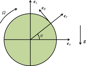
Schematic diagram of the cylindrical container, of radius
 $R$
, rotating with angular velocity
 ${\rm\Omega}$
about a horizontal axis. Cartesian and cylindrical coordinate vectors are indicated.

The proposed experimental set-up consists of a circular cylindrical chamber of radius
 $R$
rotating at a constant angular velocity
 ${\rm\Omega}$
about a horizontal axis (figure 1); this arrangement is sometimes called a clinostat. The chamber is filled with a dilute suspension of gyrotactic cells (e.g. C. nivalis or C. reinhardtii), of average number density
 $n_{0}$
. The chamber is relatively narrow in the axial direction, so that flow will be approximately two-dimensional, but wide enough that sidewall effects are unimportant in the neighbourhood of the centre plane where observation is made. It is assumed that the suspension is illuminated with light from which wavelengths to which the cells are sensitive have been filtered, thus ruling out phototaxis. In fact, such an experiment has previously been set up by Kessler et al. (Reference Kessler, Hill, Strittmatter and Wiseley1998) in order to investigate individual trajectories of Pleurochrysis carterae; here, the chamber had a radius
 $R$
of 5 mm and a width
 $w$
of 1 mm; the reported rotation rates were in the range
 $0.3{-}1.0\ \text{rad}\ \text{s}^{-1}$
. New experiments are also currently being performed with C. reinhardtii cells and spherical colonies of Volvox carteri, by S. Furlan and R. E. Goldstein (personal communication), with
 $R=$
20 mm,
 $w=5\ \text{mm}$
and
 ${\rm\Omega}$
in the range
 $0{-}10^{\circ }\ \text{s}^{-1}$
, i.e.
 $0{-}0.17\ \text{rad}\ \text{s}^{-1}$
. The difference between the present proposed experiment and these predecessors is the intention to investigate suspensions rather than individual cells, at least for Chlamydomonas (Volvox colonies are much larger).
2. Theory
In the laboratory frame of reference, sketched in figure 1, the velocity field of the background solid-body rotation is
 $$\begin{eqnarray}\boldsymbol{u}=-{\rm\Omega}r\boldsymbol{e}_{{\it\theta}},\end{eqnarray}$$
with vorticity
 $$\begin{eqnarray}{\bf\omega}=2{\rm\Omega}\boldsymbol{e}_{y}\end{eqnarray}$$
and zero strain rate. Here,
 $(r,{\it\theta})$
are plane polar coordinates; the
 $y$
-axis is perpendicular to the plane of the flow. We assume that perturbations to the flow field resulting from density variations are small, so that the only property of the flow that influences the probability density function (p.d.f.) of swimming direction,
 $f(\,\boldsymbol{p})$
, is the background vorticity; because the strain rate is identically zero, the Fokker–Planck equation (1.5) is the same for non-spherical as for spherical cells. We shall assume steady flow and steady cell concentration distribution.
The theory will proceed in three steps. First, solve (1.5) for
 $f(\,\boldsymbol{p})$
and use the result to compute the mean cell swimming velocity
 $\boldsymbol{V}_{C}$
from (1.6). Second, using the result for
 $\boldsymbol{V}_{C}$
, calculate
 $n(\boldsymbol{x})$
from the time-independent version of (1.1), assuming that the perturbation to the background flow can be neglected. Third, calculate the perturbation to the background flow by solving the Navier–Stokes equations (1.9) and (1.10). It should be noted that the perturbation is a necessary consequence of gravity acting on the predicted variations in cell concentration, not of an instability as in bioconvection.
In terms of spherical polar coordinates in orientation space,
 $({\it\chi},{\it\phi})$
, where
 ${\it\chi}=0$
is vertically upwards (parallel to
 $\boldsymbol{e}_{z}$
) and
 ${\it\phi}=0$
is in the horizontal
 $x$
-direction, (1.5) is
 $$\begin{eqnarray}\displaystyle & & \displaystyle BD_{R}\left[\frac{1}{\sin {\it\chi}}\frac{\partial }{\partial {\it\chi}}\left(\sin {\it\chi}\frac{\partial f}{\partial {\it\chi}}\right)+\frac{1}{\sin ^{2}{\it\chi}}\frac{\partial ^{2}f}{\partial {\it\phi}^{2}}\right]+\left(\sin {\it\chi}\frac{\partial f}{\partial {\it\chi}}+2\cos {\it\chi}f\right)\nonumber\\ \displaystyle & & \displaystyle \quad =B{\rm\Omega}\left(\cos {\it\phi}\frac{\partial f}{\partial {\it\chi}}-\cot {\it\chi}\sin {\it\phi}\frac{\partial f}{\partial {\it\phi}}\right)\!,\end{eqnarray}$$
to be solved subject to the normalisation condition
 $$\begin{eqnarray}\iint f\sin {\it\chi}\text{d}{\it\chi}\text{d}{\it\phi}=1.\end{eqnarray}$$
Since the background flow is two-dimensional,
 $f$
will be an even function of
 ${\it\phi}$
and
 $\langle p_{y}\rangle =0$
. Moreover, since the flow is uniform across the cylinder,
 $\langle \,\boldsymbol{p}\rangle$
will also be uniform. Hence, the average cell swimming velocity (1.6) will take the form
 $$\begin{eqnarray}\boldsymbol{V}_{C}=V_{C}\langle \,\boldsymbol{p}\rangle =(V_{x},0,V_{z}),\end{eqnarray}$$
where
 $V_{x},V_{z}$
are constants and, for example,
 $$\begin{eqnarray}V_{x}=V_{C}\int _{0}^{2{\rm\pi}}\int _{0}^{{\rm\pi}}\sin ^{2}{\it\chi}\sin {\it\phi}f({\it\chi},{\it\phi})\text{d}{\it\chi}\text{d}{\it\phi}.\end{eqnarray}$$
The Fokker–Planck equation (2.3) was solved for this case (two-dimensional, uniform vorticity) by Bees, Hill & Pedley (Reference Bees, Hill and Pedley1998), who wrote
 $f$
as an infinite series of spherical harmonics whose coefficients were computed numerically. The equation has also been solved numerically by Hwang & Pedley (Reference Hwang and Pedley2014). If required, one can use their results to obtain values for
 $V_{x}$
and
 $V_{z}$
directly (see figure 3 of Hwang & Pedley Reference Hwang and Pedley2014, for example).
Here, we merely present the analysis for large rotation rate,
 $B{\rm\Omega}\gg 1$
, when vorticity dominates gravity in (2.3): the swimming cells are all tumbling. We assume
 $BD_{R}=O(1)$
and seek a solution of the form
 $$\begin{eqnarray}f=\frac{1}{4{\rm\pi}}+\frac{1}{B{\rm\Omega}}\,f_{1}({\it\chi},{\it\phi})+\frac{1}{(B{\rm\Omega})^{2}}\,f_{2}({\it\chi},{\it\phi})+O[(B{\rm\Omega})^{-3}].\end{eqnarray}$$
Substitution in (2.3) then yields
 $$\begin{eqnarray}f_{1}=\frac{1}{2{\rm\pi}}\sin {\it\chi}\cos {\it\phi},\quad f_{2}=\frac{1}{2{\rm\pi}}\left(-\frac{1}{4}-\frac{3}{4}\cos 2{\it\chi}+2BD_{R}\cos {\it\chi}\right),\end{eqnarray}$$
so, from (1.7),
 $$\begin{eqnarray}\langle \,\boldsymbol{p}\rangle =\frac{2}{3B{\rm\Omega}}\left(\boldsymbol{e}_{x}+\frac{2D_{R}}{{\rm\Omega}}\boldsymbol{e}_{z}\right),\quad \text{i.e.}\ V_{x}=\frac{2V_{C}}{3B{\rm\Omega}},\ V_{z}=\frac{4D_{R}}{3B{\rm\Omega}^{2}}.\end{eqnarray}$$
The mean swimming velocity is thus horizontal to leading order. The result (2.9) was previously reported by Bees et al. (Reference Bees, Hill and Pedley1998); similar results were obtained in a study of three-dimensional flows by Thorn & Bearon (Reference Thorn and Bearon2010).
We write the steady dimensionless version of (1.1) in plane polar coordinates
 $(Rr,{\it\theta})$
(figure 1), as follows:
 $$\begin{eqnarray}\displaystyle & & \displaystyle \frac{\partial ^{2}n}{\partial r^{2}}+\frac{1}{r}\frac{\partial n}{\partial r}+\frac{1}{r^{2}}\frac{\partial ^{2}n}{\partial {\it\theta}^{2}}+{\it\beta}^{2}\frac{\partial n}{\partial {\it\theta}}\nonumber\\ \displaystyle & & \displaystyle \quad ={\it\alpha}\left(\cos {\it\theta}\frac{\partial n}{\partial r}-\frac{\sin {\it\theta}}{r}\frac{\partial n}{\partial {\it\theta}}\right)+{\it\gamma}\left(\sin {\it\theta}\frac{\partial n}{\partial r}+\frac{\cos {\it\theta}}{r}\frac{\partial n}{\partial {\it\theta}}\right)\!,\end{eqnarray}$$
where we have assumed that the cell translational diffusivity is isotropic (
 $=D$
) and the dimensionless constants
 ${\it\alpha},{\it\beta},{\it\gamma}$
are defined as follows:
 $$\begin{eqnarray}{\it\alpha}=\frac{V_{x}R}{D},\quad {\it\beta}^{2}=\frac{{\rm\Omega}R^{2}}{D},\quad {\it\gamma}=\frac{(V_{z}-V_{G})R}{D}.\end{eqnarray}$$
Thus,
 ${\it\alpha}$
is the Péclet number based on the horizontal component of the cell swimming velocity (from (1.6) and (2.5)),
 ${\it\beta}^{2}$
is the Péclet number based on the rotation rate of the chamber and
 ${\it\gamma}$
is the Péclet number based on the vertical component of the average cell swimming velocity combined with the cell sedimentation speed.
The boundary condition on
 $n$
is that of zero flux at the cylinder wall:
 $$\begin{eqnarray}\frac{\partial n}{\partial r}-{\it\alpha}n\cos {\it\theta}-{\it\gamma}n\sin {\it\theta}=0.\end{eqnarray}$$
It can be seen that, since
 $n=\text{const.}$
is a solution of (2.10), the only reason for there to be variations in
 $n$
is the boundary condition (2.12) – swimming or sedimenting to the wall causes a build-up of cells there.
Independently of the assumption
 $B{\rm\Omega}\gg 1$
, we now also assume that
 ${\it\beta}\gg 1$
. It then appears that the build-up (or depletion) of cells near the wall will take place in a thin boundary layer, of thickness proportional to
 ${\it\beta}^{-1}$
. In this boundary layer the normal diffusion of cells, non-uniform in the azimuthal direction, will be limited by advection with the background rotation. We therefore set
 $$\begin{eqnarray}{\it\eta}={\it\beta}(1-r)\end{eqnarray}$$
and seek a solution of the form
 $$\begin{eqnarray}n=1+\frac{1}{{\it\beta}}n_{1}({\it\eta},{\it\theta})+O({\it\beta}^{-2}).\end{eqnarray}$$
Substitution in (2.10) and (2.12) gives the following equation and boundary condition for
 $n_{1}$
:
 $$\begin{eqnarray}\frac{\partial ^{2}n_{1}}{\partial {\it\eta}^{2}}+\frac{\partial n_{1}}{\partial {\it\theta}}=0;\quad \frac{\partial n_{1}}{\partial {\it\eta}}=-{\it\alpha}\cos {\it\theta}-{\it\gamma}\sin {\it\theta}\quad \text{on}\;{\it\eta}=0,\end{eqnarray}$$
and we assume in addition that
 $n_{1}\rightarrow 0$
as
 ${\it\eta}\rightarrow \infty$
. The solution is easily obtained as
 $$\begin{eqnarray}n_{1}=({\it\alpha}^{2}+{\it\gamma}^{2})^{1/2}\exp \left(-\frac{{\it\eta}}{\sqrt{2}}\right)\cos \left({\it\theta}-{\it\theta}_{0}+\frac{{\rm\pi}}{4}+\frac{{\it\eta}}{\sqrt{2}}\right),\end{eqnarray}$$
where
 $$\begin{eqnarray}\tan {\it\theta}_{0}=\frac{{\it\gamma}}{{\it\alpha}}.\end{eqnarray}$$
It can be seen that the concentration at the wall exhibits a
 ${\rm\pi}/4$
phase lag behind its gradient at the wall. This is to be expected, since the problem (2.15a,b
) is the same as that of heat diffusion in a semi-infinite medium when the heat flux at the surface is a periodic function of time, with time replaced by
 $-{\it\theta}$
(Carslaw & Jaeger Reference Carslaw and Jaeger1959).
The cell concentration distribution given by (2.14) and (2.16) is non-uniform in the boundary layer of thickness
 ${\it\beta}^{-1}$
. There will therefore be a perturbation to the background flow, which can also be analysed under the boundary-layer approximation. Assuming no Rayleigh–Taylor instability (bioconvection), the component of the equation of motion perpendicular to the boundary (i.e. radial) reduces to
 $\partial p/\partial {\it\eta}=0$
, where
 $p$
is the dimensionless pressure, so
 $p$
is approximately uniform everywhere. If we write the
 ${\it\theta}$
-component of the velocity as
 $-{\rm\Omega}r+u_{{\it\theta}}$
, the
 ${\it\theta}$
-component of the equation of motion becomes
 $$\begin{eqnarray}{\it\mu}\frac{\partial ^{2}u_{{\it\theta}}}{\partial {\it\eta}^{2}}=\frac{{\bar{g}}{\it\rho}R^{2}}{{\it\beta}^{3}}n_{1}\cos {\it\theta},\end{eqnarray}$$
where
 ${\bar{g}}=n_{0}g{\it\upsilon}{\rm\Delta}{\it\rho}/{\it\rho}$
and
 ${\it\upsilon}$
is the volume of a cell. Equation (2.18) must be solved subject to the boundary conditions
 $$\begin{eqnarray}u_{{\it\theta}}=0\quad \text{at}\;{\it\eta}=0;\quad \frac{\partial u_{{\it\theta}}}{\partial {\it\eta}}\rightarrow 0\quad \text{as}\;{\it\eta}\rightarrow \infty ,\end{eqnarray}$$
and the solution is
 $$\begin{eqnarray}u_{{\it\theta}}={\rm\Omega}Ru_{0}\cos {\it\theta}\,\text{Re}\left(-\text{i}\exp [\text{i}({\it\theta}-{\it\theta}_{0}+{\rm\pi}/4)]\left[1-\exp \left(\frac{-(1-\text{i}){\it\eta}}{\sqrt{2}}\right)\right]\right)\!,\end{eqnarray}$$
where
 $$\begin{eqnarray}u_{0}=\frac{({\it\alpha}^{2}+{\it\gamma}^{2})^{1/2}R{\bar{g}}}{{\it\beta}^{3}{\it\nu}{\rm\Omega}}.\end{eqnarray}$$
The above result shows that the tangential velocity perturbation does not tend to zero as
 ${\it\eta}\rightarrow \infty$
. Thus, it drives a perturbation to the solid-body rotation in the core outside the boundary layer, which we proceed to calculate. Let the fluid velocity in the core be
 ${\rm\Omega}R(u_{0}u,-r+u_{0}v,0)$
, in cylindrical polar coordinates
 $(Rr,{\it\theta},y)$
. This flow field will satisfy the boundary conditions at
 $r=1$
of no penetration and slip velocity given by (2.20), i.e.
 $$\begin{eqnarray}\displaystyle & u(r=1)=0, & \displaystyle\end{eqnarray}$$
 $$\begin{eqnarray}\displaystyle & v(r=1)=\cos {\it\theta}\sin ({\it\theta}-{\it\theta}_{0}+{\rm\pi}/4)={\textstyle \frac{1}{2}}[\sin (2{\it\theta}-{\it\theta}_{0}+{\rm\pi}/4)-\sin ({\it\theta}_{0}-{\rm\pi}/4)].\qquad & \displaystyle\end{eqnarray}$$
 $u_{0}\ll 1$
, then, with a suitably rescaled pressure perturbation, the Navier–Stokes and continuity equations in
 $0\leqslant r<1$
become
 $$\begin{eqnarray}\displaystyle & \displaystyle Re\left(-\frac{\partial u}{\partial {\it\theta}}+2v\right)=-\frac{\partial p}{\partial r}+\left({\rm\nabla}^{2}u-\frac{u}{r^{2}}-\frac{2}{r^{2}}\frac{\partial v}{\partial {\it\theta}}\right), & \displaystyle\end{eqnarray}$$
 $$\begin{eqnarray}\displaystyle & \displaystyle Re\left(-2u-\frac{\partial v}{\partial {\it\theta}}\right)=-\frac{1}{r}\frac{\partial p}{\partial {\it\theta}}+\left({\rm\nabla}^{2}v-\frac{v}{r^{2}}+\frac{2}{r^{2}}\frac{\partial u}{\partial {\it\theta}}\right), & \displaystyle\end{eqnarray}$$
 $$\begin{eqnarray}\displaystyle & \displaystyle \frac{1}{r}\frac{\partial (ru)}{\partial r}+\frac{1}{r}\frac{\partial v}{\partial {\it\theta}}=0, & \displaystyle\end{eqnarray}$$
 $$\begin{eqnarray}Re=\frac{{\rm\Omega}R^{2}}{{\it\nu}}.\end{eqnarray}$$
The continuity equation (2.24c ) implies the existence of a stream function, and the boundary condition (2.23) then suggests that we write
 $$\begin{eqnarray}u=-\frac{1}{r}\frac{\partial {\it\psi}}{\partial {\it\theta}},\quad v=-\frac{r}{2}\sin ({\it\theta}_{0}-{\rm\pi}/4)+\frac{\partial {\it\psi}}{\partial r},\end{eqnarray}$$
where
 $$\begin{eqnarray}{\it\psi}=f(r)\exp \text{i}(2{\it\theta}-{\it\theta}_{0}-{\rm\pi}/4)\end{eqnarray}$$
(real parts being assumed) and
 $$\begin{eqnarray}f(1)=0,\quad f^{\prime }(1)=-\text{i}/2.\end{eqnarray}$$
The equation for
 $f(r)$
, from (2.24), is
 $$\begin{eqnarray}f^{\prime \prime \prime \prime }+\frac{2}{r}\,f^{\prime \prime \prime }-\frac{9}{r^{2}}\,f^{\prime \prime }+\frac{9}{r^{3}}\,f^{\prime }=-2\text{i}Re\left(f^{\prime \prime }+\frac{f^{\prime }}{r}-\frac{4f}{r^{2}}\right)\!,\end{eqnarray}$$
with the boundary conditions (2.28a,b
) supplemented by the requirement that
 $f(r)$
be bounded at
 $r=0$
. The solution is
 $$\begin{eqnarray}f(r)=-\frac{\text{i}}{2}\frac{r^{2}\text{J}_{2}({\it\lambda})-\text{J}_{2}({\it\lambda}r)}{{\it\lambda}\text{J}_{3}({\it\lambda})},\end{eqnarray}$$
where
 ${\it\lambda}^{2}=2\text{i}Re$
and
 $\text{J}_{2}$
,
 $\text{J}_{3}$
are Bessel functions. When
 $Re$
is small, (2.27) and (2.30) reduce to
 $$\begin{eqnarray}{\it\psi}=-{\textstyle \frac{1}{4}}r^{2}(1-r^{2})\sin (2{\it\theta}-{\it\theta}_{0}+{\rm\pi}/4),\end{eqnarray}$$
which could be obtained directly from the Stokes equations. When
 $Re$
is large, the core flow itself has the form of a boundary layer, with only solid-body rotation in the centre of the cylinder. In this limit, the tangential component of perturbed velocity,
 $v$
, becomes
 $$\begin{eqnarray}v\approx -\frac{r}{2}\sin ({\it\theta}_{0}-{\rm\pi}/4)-\frac{1}{2\sqrt{r}}\exp \left[-\sqrt{Re}(1-r)\right]\sin \left[2{\it\theta}-{\it\theta}_{0}+{\rm\pi}/4+\sqrt{Re}(1-r)\right].\end{eqnarray}$$
3. Results and parameter values
The angle
 ${\it\theta}_{0}$
is given by (2.17), and represents the direction of the average velocity of the cells in the core of the cylinder, due to both swimming and sedimentation, relative to the basic solid-body rotation. However, its value does not affect the structure of the cell concentration distribution (2.16) or the resulting perturbation to the flow, given by (2.20) and (2.30). Hence, we plot the perturbation flow for the case
 ${\it\theta}_{0}=0$
; the flow pattern is merely rotated for other values of
 ${\it\theta}_{0}$
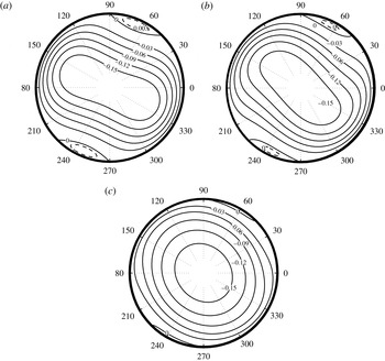
. Streamlines are plotted in figure 2 for
 $Re=0,20$
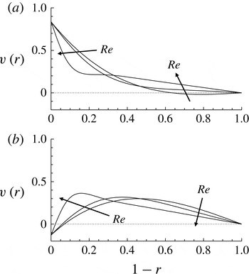
and 200, and in figure 3 we plot profiles of the tangential velocity outside the concentration boundary layer, given by (2.26a,b
), (2.27) and (2.30), for the same values of
 $Re$
. The predicted boundary-layer structure can be seen at the largest value of
 $Re$
.


Profiles of the perturbed tangential velocity outside the concentration boundary layer at two angular locations ((a)
 ${\it\theta}=60^{\circ }$
and (b)
 ${\it\theta}=150^{\circ }$
) for the same three values of the Reynolds number as in figure 2.

It should be remembered that the plotted flow is a perturbation from the background solid-body rotation, so could only be directly observed if one used a co-rotating camera. From a laboratory-based perspective only the radial component of this motion is likely to be directly visible, although tangential velocity measurements could be made to check the predictions quantitatively. A further test, if it were possible, would be to measure the cell concentration distribution in the boundary layer.
In order to assess the validity of the approximations made in the analysis, notably
 ${\it\beta}\gg 1,u_{0}\ll 1$
and, perhaps,
 $B{\rm\Omega}\gg 1$
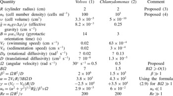
, we provide estimates of the parameter values for two possible experiments, one with Volvox and one with Chlamydomonas reinhardtii. These are listed in table 1; relevant data on Volvox come from Drescher et al. (Reference Drescher, Leptos, Tuval, Ishikawa, Pedley and Goldstein2009) and on Chlamydomonas from Kessler (Reference Kessler1985, Reference Kessler1986) and S. Furlan and R. E. Goldstein (personal communication). From these data it is clear that the assumptions
 ${\it\beta}\gg 1$
and
 $u_{0}\ll 1$
are valid in both cases; it is less clear that
 $B{\rm\Omega}\gg 1$
but, as pointed out above, this assumption is required only for deriving analytical expressions for the components
 $V_{x},V_{z}$
of the mean cell swimming velocity, as in (2.9). Since these components do not vary with position, they have influence only through the values of the parameters
 ${\it\alpha}$
and
 ${\it\gamma}$
, as in (2.11a−c
). The parameter values given in table 1 show that both
 ${\it\beta}$
and
 $u_{0}^{-1}$
are very large, while
 $B{\rm\Omega}$
is not. The effective Reynolds number
 $Re$
of the flow perturbation is in both cases approximately 200, the value for which the results are given in figures 2(c) and 3, so these should be observable, after rotation through an angle
 ${\it\theta}_{0}$
.
Parameter values, actual or proposed. (1) Volvox data are based on a colony of radius
 $200\ {\rm\mu}\text{m}$
(Drescher et al.
Reference Drescher, Leptos, Tuval, Ishikawa, Pedley and Goldstein2009). (2) Chlamydomonas data are taken from Kessler (Reference Kessler1986) and Hill & Häder (Reference Hill and Häder1997). (3) The proposed radius and rotation rate are based on what is currently achievable in the apparatus of S. Furlan and R. E. Goldstein (personal communication). (4) For Chlamydomonas,
 $n_{0}$
is chosen to be lower than the values for which Kessler (Reference Kessler1985) observed bioconvection.

A further assumption implicit in the continuum model is that all length scales in the analysis are large compared with the micro-organism size and spacing. This may be questionable in the boundary layer, whose thickness is
 ${\it\beta}^{-1}R$
, which has the value
 $52\ {\rm\mu}\text{m}$
for the proposed Chlamydomonas experiments and
 $14\ {\rm\mu}\text{m}$
for the Volvox experiments, from table 1 (the smallness of the value for Volvox is a consequence of the very small value taken for
 $D$
). The former is significantly larger than the length of a single cell (
 ${\approx}10\ {\rm\mu}\text{m}$
), but may not be much larger than the spacing. Therefore, the details of how cells interact with a rigid boundary may become important, although they would not affect the boundary condition (2.12) unless they stuck to the boundary (see Kantsler et al.
Reference Kantsler, Dunkel, Polin and Goldstein2013). A length of
 $14\ {\rm\mu}\text{m}$
is definitely smaller than the radius of any Volvox colony, so experiments with Volvox will have to remain confined to measurements of individual colonies, not suspensions. In the case of Chlamydomonas, the boundary-layer thickness could be increased by decreasing the angular velocity
 ${\rm\Omega}$
.
Yet another assumption is that the effect of the flow perturbation is negligible in (1.1), while that of the cell swimming and sedimentation is not. In the case of Volvox,
 $u_{0}{\rm\Omega}R$
is approximately
 $3\times 10^{-5}\ \text{cm s}^{-1}$
, much less than
 $V_{C}$
(
 ${\approx}0.02\ \text{cm s}^{-1}$
). In the case of Chlamydomonas, however,
 $u_{0}{\rm\Omega}R\approx 0.02\ \text{cm s}^{-1}$
, approximately ten times larger than
 $V_{C}$
. In order to reduce
 $u_{0}$
, it would be necessary to reduce the cell number density
 $n_{0}$
– at the risk of increasing the cell spacing. When an experiment is running, it may prove necessary to solve the nonlinear problem in which the perturbation velocity is not neglected in (1.1).
Acknowledgements
The author would like to express his gratitude to Dr Y. Hwang for insightful conversations and help in plotting the figures, and to S. Furlan and R. E. Goldstein for sharing their experimental plans.