





Impact Statement
This work advances negligible-mean-flow turbulence research through a symmetric two-panel facility based on true synthetic jets with independently tuneable power, frequency and activation. An extended sunbathing strategy beyond conventional on/off forcing enables dynamic control of turbulence statistics and systematic exploration of forcing parameter space. A key contribution is the identification and quantification of facility-induced coherent structures and their energetic content, providing an additional framework for characterising turbulence facilities beyond conventional statistics alone. Spatial power gradient enables controlled large-scale mean-flow rotation without mechanical rotation, providing a compact platform for systematically investigating turbulence under rotational effects. The facility provides a versatile platform for experimental fluid mechanics studies, including validation of theoretical and numerical models.
1. Introduction
Turbulent flows consist of irregular, multiscale motions in which energy is transferred from large to small scales and ultimately dissipated by viscosity (Frisch Reference Frisch1995; Kolmogorov Reference Kolmogorov1941; Pope Reference Pope2000). Turbulence is often generated by shear in the mean flow, where velocity gradients supply energy to the fluctuations, with production balancing dissipation in statistically steady conditions (Hinze Reference Hinze1975; Pope Reference Pope2000). When velocity fluctuation statistics are directionally invariant, the flow is termed isotropic and when they are spatially uniform, it is homogeneous (Batchelor Reference Batchelor1953). While most natural and engineering flows deviate from these ideal conditions, homogeneous isotropic turbulence (HIT) provides a canonical framework for studying fundamental turbulence.
HIT with negligible mean flow represents a canonical turbulent state that is statistically uniform and rotationally invariant. Laboratory realisations of negligible-mean-flow HIT are particularly valuable for advancing fundamental turbulence research, as they eliminate confounding influences such as mean shear, boundary layers and large-scale advection. These idealised conditions enable direct investigation of intrinsic turbulence dynamics and provide critical benchmarks for theoretical models, including Kolmogorov similarity hypotheses (Batchelor Reference Batchelor1953; Lawson et al. Reference Lawson, Bodenschatz, Knutsen, Dawson and Worth2019; Marston & Tobias Reference Marston and Tobias2023). Negligible-mean-flow configurations are also advantageous for Lagrangian measurements, allowing tracer particles to remain within a fixed measurement volume for extended durations, thereby enabling long-time statistics such as single-particle and pair dispersion. Similarly, Eulerian measurements of inertial particle settling, clustering, and collision statistics benefit from the absence of strong mean convection (Good et al. Reference Good, Ireland, Bewley, Bodenschatz, Collins and Warhaft2014; Petersen et al. Reference Petersen, Baker and Coletti2019). Motivated by these advantages, a wide range of laboratory facilities have been developed to generate negligible-mean-flow HIT. A detailed overview of facilities for negligible-mean-flow HIT is given in the recent review by Ghazi Nezami et al. (Reference Ghazi Nezami, Byron and Johnson2023). Now, we briefly describe these HIT facilities to introduce the key concepts.
Early efforts to approximate HIT led to the development of grid-stirred tanks (GSTs), in which a planar grid oscillates normal to its plane within a confined tank (Rouse & Dodu Reference Rouse and Dodu1955). Interactions between wakes generated during successive grid strokes produce approximately homogeneous turbulence away from the grid. While two-grid symmetric configurations improve isotropy relative to single-grid systems (Blum et al. Reference Blum, Kunwar, Johnson and Voth2010; Srdic et al. Reference Srdic, Fernando and Montenegro1996), GSTs remain susceptible to spatial decay, sensitive to grid position and allow the development of large-scale circulation driven by mass conservation within confined geometries (Dohan & Sutherland Reference Dohan and Sutherland2002; McKenna & McGillis Reference McKenna and McGillis2004). Even multi-grid systems cannot fully suppress these recirculations (Blum et al. Reference Blum, Kunwar, Johnson and Voth2010). Moreover, oscillatory grid motion introduces coherent large-scale motions that contaminate the intended HIT field and limit achievable turbulence intensity (Variano & Cowen Reference Variano and Cowen2008). Mean flow magnitudes approaching 30% of the root-mean-square velocity have been reported in several GST studies (Huang et al. Reference Huang, Lv, Chen, Song, Yin and Wang2024; McKenna & McGillis Reference McKenna and McGillis2004).
Synthetic jets offer an alternative approach for generating energetic turbulence with minimal mean flow. By periodically ingesting and expelling fluid through an orifice using loudspeakers, diaphragms or piezoelectric actuators, synthetic jets inject momentum without net mass flux (Smith & Glezer Reference Smith and Glezer1998). The resulting vortex rings and jet–jet interactions generate strong turbulence while largely suppressing background mean motion. Distributed synthetic jets have been used to create central regions of near-HIT with improved scale separation relative to grid-based methods.
Several facilities have exploited this concept. Hwang & Eaton (Reference Hwang and Eaton2004) demonstrated that inward-facing loudspeakers mounted at the corners of a cubic chamber generate nearly isotropic turbulence. Variants of this design have been used to study plankton dynamics (Webster et al. Reference Webster, Brathwaite and Yen2004), Lagrangian particle tracking (Lu et al. Reference Lu, Fugal, Nordsiek, Saw, A Shaw and Yang2008) and particle dispersion (Sabban & van Hout, Reference Sabban and van Hout2011; Sabban et al. Reference Sabban, Cohen and van Hout2017). Larger-volume facilities employing truncated-icosahedral geometries have further expanded the accessible homogeneous region (Bewley et al. Reference Bewley, Chang and Bodenschatz2012, Reference Bewley, Saw and Bodenschatz2013; Chang et al. Reference Chang, Bewley and Bodenschatz2012). More recently, Hoffman & Eaton (Reference Hoffman and Eaton2021) developed a vertical loudspeaker array for air turbulence, providing scaling arguments for achieving target Reynolds numbers and dissipation rates. Despite these advances, synthetic-jet facilities often suffer from small homogeneous regions, geometric asymmetries and difficulties in maintaining negligible mean flow at high turbulence intensities (Hoffman & Eaton Reference Hoffman and Eaton2021; Ghazi Nezami et al. Reference Ghazi Nezami, Byron and Johnson2023).
An alternative strategy employs pump-driven or valve-based jets, commonly referred to as quasi-synthetic jets, arranged in planar arrays known as randomly actuated jet arrays (RJAs). Although these systems lack true suction–ejection cycles, they can approximate zero-net-mass-flux forcing while offering flexible spatiotemporal control (Bellani & Variano Reference Bellani and Variano2014; Carter et al. Reference Carter, Petersen, Amili and Coletti2016; Esteban et al. Reference Esteban, Shrimpton and Ganapathisubramani2019; Masuk et al. Reference Masuk, Salibindla, Tan and Ni2019; Variano et al. Reference Variano, Bodenschatz and Cowen2004). In RJAs, jets are stochastically actuated to suppress persistent mean recirculation and generate homogeneous turbulence away from the forcing planes. Variations of these facilities include the corner-jet-symmetric configuration introduced by McCutchan & Johnson (Reference McCutchan and Johnson2023), in which jets are positioned at the corners and edge midpoints of a cubic chamber. Symmetric multi-panel configurations (Bang & Pujara Reference Bang and Pujara2023; Bellani & Variano Reference Bellani and Variano2014; Carter et al. Reference Carter, Petersen, Amili and Coletti2016), as well as corner-jet-symmetric arrangements (McCutchan & Johnson Reference McCutchan and Johnson2023), have demonstrated improved isotropy and homogeneity compared with conventional single-panel configurations.
The RJAs are typically operated using the sunbathing algorithm, introduced by Variano & Cowen (Reference Variano and Cowen2008). In this scheme, each jet is switched on and off for durations
 $T_{\mathrm{on}}$
and
 $T_{\mathrm{off}}$
drawn from Gaussian distributions with prescribed means
 $(\mu _{\mathrm{on}},\mu _{\mathrm{off}})$
and variances
 $(\sigma _{\mathrm{on}}^{2},\sigma _{\mathrm{off}}^{2})$
. Following an initial operation period, the fraction of jets active at any instant converges towards the source fraction
 $\phi _{\mathrm{on}}\equiv \mu _{\mathrm{on}}/(\mu _{\mathrm{on}}+\mu _{\mathrm{off}})$
. This approach significantly reduces mean flow relative to deterministic forcing and enables homogeneous regions exceeding the integral scale. Variano & Cowen (Reference Variano and Cowen2008) demonstrated that, in single-panel arrays, the root-mean-square velocity is maximised at
 $\phi _{\mathrm{on}} \approx 12.5\,\%$
and the optimum standard deviations provided
 $\sigma _{\mathrm{on}} /\mu _{\mathrm{on}}\approx 1/3$
. Subsequent studies demonstrated that turbulence intensity and Reynolds number could be tuned by adjusting actuation parameters such as mean on-time (Carter et al. Reference Carter, Petersen, Amili and Coletti2016; Pérez-Alvarado et al. Reference Pérez-Alvarado, Mydlarski and Gaskin2016; Johnson & Cowen Reference Johnson and Cowen2018).
Although there are multiple parameters (source fraction, standard deviation and mean on/off time), most studies set the first two at 12.5 % and 1/3 while only varying mean on/off time. Moreover, most RJAs are driven by bilge pumps operated at constant velocity to reduce wear (Bang & Pujara Reference Bang and Pujara2023; Bellani & Variano Reference Bellani and Variano2014; Esteban et al. Reference Esteban, Shrimpton and Ganapathisubramani2019; Variano & Cowen Reference Variano and Cowen2008; Johnson & Cowen Reference Johnson and Cowen2018; Ghazi Nezami & Johnson Reference Ghazi Nezami and Johnson2024; Pérez-Alvarado et al. Reference Pérez-Alvarado, Mydlarski and Gaskin2016) or by similarly constant choked jets (Carter et al. Reference Carter, Petersen, Amili and Coletti2016), significantly limiting the level of control over actuation. To address this limitation, several water-based facilities introduced variable forcing intensity. The centre-facing nonplanar arrangement of McCutchan & Johnson (Reference McCutchan and Johnson2023) and the asymmetric planar configuration of Pratt et al. (Reference Pratt, True and Crimaldi2017) employed variable-voltage control to modify the jet velocity. These studies demonstrated that increasing jet velocity increased turbulence intensity. However, the turbulence characteristics were adjusted only between discrete operating conditions rather than through continuous modulation within a single experiment. In a symmetric planar jet facility without synthetic jets, Lawson & Ganapathisubramani (Reference Lawson and Ganapathisubramani2022) partially addressed this limitation by using impellers capable of reverse rotation, enabling velocity variation while retaining sunbathing-style randomisation. Nevertheless, the resulting flow exhibited relatively large mean circulation and anisotropy.
True synthetic-jet facilities, by contrast, offer direct control over HIT through power input and spatial frequency modulation (Hoffman & Eaton Reference Hoffman and Eaton2021). Previous studies have primarily varied these parameters between operating conditions to control the resulting turbulence characteristics. However, such facilities have generally employed continuous operation of all jets (
 $\phi _{\mathrm{on}}=100\,\%$
), without sunbathing-type partial firing or dynamic multi-parameter stochastic modulation. Consequently, the combined benefits of planar symmetric RJA geometries and the actuation flexibility of true synthetic jets have not yet been fully realised. The present facility extends this capability by dynamically varying jet velocity and frequency during operation, in addition to intermittent jet activation.
Turbulent kinetic energy spectrum consists of contributions from both large- and small-scale motions (Pope Reference Pope2000), where the large-scale component often contains spatially or temporally organised motions commonly referred to as coherent structures. Examples include vortices, circulation cells, shear-layer structures, low-frequency oscillations, jet interactions and large-scale recirculating motions. These structures are commonly generated by the forcing strategy and geometry of the flow facility. Temporal organisation is commonly observed in oscillating-grid turbulence, where reproducible large-scale motions remain phase-locked to the grid oscillation (Poulain-Zarcos et al. Reference Poulain-Zarcos, Mercier and ter Halle2022). Spatial organisation, in contrast, appears as energetic flow structures that repeatedly occur at similar spatial locations within the measurement domain without requiring strict temporal periodicity (Haller Reference Haller2015; Li et al. Reference Li, Lu, Zhao, Xu and Wang2025). Consequently, even in facilities specifically designed for negligible-mean-flow turbulence, the absence of a mean flow does not guarantee the absence of large-scale flow organisation.
When a substantial fraction of the turbulent kinetic energy resides within coherent motions, turbulence statistics may become biased if the organised contribution is not properly identified and separated from the turbulence. This behaviour is analogous to the influence of amplitude and frequency modulation observed in wall-bounded turbulence (Ganapathisubramani et al. Reference Ganapathisubramani, Hutchins, Monty, Chung and Marusic2012; Mathis et al. Reference Mathis, Hutchins and Marusic2009). Moreover, coherent structures can significantly influence the physical behaviour of turbulent flows, including inertial particle transport (Huang et al. Reference Huang, Jie, Cui, Xu, Andersson and Zhao2025), scalar mixing (Fröhlich et al. Reference Fröhlich, García-Villalba and Rodi2008), entrainment (Neamtu-Halic et al. Reference Neamtu-Halic, Krug, Haller and Holzner2019), combustion (Coats Reference Coats1996), turbulence decay (Gautam & Berk Reference Gautam and Berk2026), heat transfer (Li et al. Reference Li, Yu, Wang and Xu2019) and spectral energy transfer (Wang et al. Reference Wang, Yang, Wu and Wang2021).
The presence of coherent structures is not always evident from conventional turbulence statistics alone. Facilities with similar Reynolds numbers, turbulent kinetic energy levels or spectral distributions may nevertheless exhibit fundamentally different large-scale flow organisation depending on the forcing strategy and design characteristics. As discussed by Ghazi Nezami et al. (Reference Ghazi Nezami, Byron and Johnson2023), forcing mechanisms that reduce effective randomness can promote persistent large-scale coherent structures even in nominally homogeneous turbulence facilities. While temporally organised motions have been widely recogniesd and, in some cases, explicitly removed in negligible-mean-flow turbulence studies (Poulain-Zarcos et al. Reference Poulain-Zarcos, Mercier and ter Halle2022), comparatively less attention has been devoted to spatially organised coherent motions. One notable example is the work of Pratt et al. (Reference Pratt, True and Crimaldi2017), who observed coherent structures generated by a negligible-mean-flow turbulence facility to investigate their influence on free-surface particle clustering. In grid turbulence, the influence of these spatial structures is typically mitigated by performing measurements in the far-field, typically at downstream distances greater than 30 mesh size (Mydlarski Reference Mydlarski2017). However, in confined negligible-mean-flow facilities, such large measurement distances are physically impractical.
These observations suggest that negligible-mean-flow facilities should not be characterised solely by conventional turbulence statistics, but also by the nature and energetics of the coherent structures they generate. Understanding facility-induced coherent structures is therefore essential for interpreting turbulence measurements and for using laboratory turbulence to explore realistic environmental and engineering flows.
In this work, we introduce a speaker-stirred turbulence chamber that integrates the planar symmetry of opposed jet arrays with the versatility of true synthetic jets capable of variable jet velocity, random frequency modulation and spatiotemporal on/off actuation. Three independent randomised forcing strategies – frequency modulation, power modulation and sunbathing-type activation – are implemented to systematically control turbulence intensity, homogeneity and isotropy. To our knowledge, this is the first negligible-mean-flow HIT facility employing multi-panel arrays of true synthetic jets rather than quasi-synthetic or impeller-based systems. The apparatus consists of two opposing arrays of 32 independently driven loudspeakers, each housed within a transparent cuboidal chamber, providing extensive degrees of freedom for actuation and dynamic control. Proper orthogonal decomposition (POD) was employed to identify and characterise forcing-induced coherent structures, providing additional insight into energy-containing motions in negligible-mean-flow turbulence. Additionally, by imposing controlled power gradients across the arrays, the facility enables the turbulence generation with mean-rotation without external rotation. Section 2 describes the experimental set-up, actuation algorithms and measurement methodology. The results, including single-point and multi-point statistics, coherent structure analysis and rotating turbulence, are presented in § 3, followed by discussion and conclusions in § 4.
2. Experiment and methods
2.1. Experimental apparatus
To leverage the advantages of both symmetric multi-panel jet arrays and loudspeaker-driven synthetic jet stirring, we designed and constructed a custom turbulence box, shown in Figure 1. The chamber is a cube with side length
 $0.61\,\text{m}$
. Turbulence is generated using synthetic jets formed by 64 Visaton KT 100 V, 4-inch, 4
 $\Omega$
loudspeakers mounted on two opposing faces of the cube. Each panel contains a
 $6\times 6$
array of speakers with corners missing for a total of 32 actuators per panel. The corner regions are reserved for bolting the structural frame that supports and rigidly holds the chamber assembly. Each synthetic jet is driven through a circular orifice of diameter
 $1\,\text{cm}$
, positioned concentrically with the speaker diaphragm with a centre-to-centre spacing of
 $10\,\text{cm}$
in both the horizontal and vertical directions. The repeated actuation of the diaphragms generates pulsed vortex rings that propagate towards the centre of the chamber, where they interact to produce turbulent flow. Optical access for planar PIV measurements is provided through the acrylic sidewalls and ceiling.
(a) Turbulence facility set-up; (b) schematic viewed from camera angle, along with sectional view of synthetic jet actuator.

Figure 1 Long description
Panel A: A 3D diagram of a turbulence facility setup. A laser and optics are directed towards a speaker’s panel, with a camera positioned to capture the scene. The setup includes multiple rows of speakers. Panel B: A schematic view from the camera angle, showing a rectangular grid with six rows and multiple columns of synthetic jet actuators. The grid dimensions are 610 millimeters in width and height, with each actuator spaced 102 millimeters apart. A sectional view of a synthetic jet actuator is also provided, showing internal components and dimensions.
Each loudspeaker is driven independently, providing full spatiotemporal control of the forcing. A Python-based control programme running on a PC generates user-defined actuation signals in the form of square waves, which are routed to a LabJack U6 digital-to-analogue converter (DAC). The DAC outputs sinusoidal voltage signals that are amplified by multichannel power amplifiers and supplied to the 64 loudspeakers. The input voltage amplitude is adjustable up to
 $2.5\,\mathrm{V}$
, which is amplified to match the speaker rating of
 $25\,\mathrm{W}$
. Actuation frequencies of up to
 $44\,\mathrm{Hz}$
are achievable and are limited by the DAC update time, which requires approximately
 $11.5\,\mathrm{ms}$
to update a single voltage value. As a result, the available actuation frequencies are discrete and correspond to divisors of
 $44\,\mathrm{Hz}$
. The loudspeakers have a resonant frequency of approximately
 $42\,\mathrm{Hz}$
and the electrical power consumption varies slightly with actuation frequency. The power consumption was measured by the root-mean-square voltage obained at the speaker terminal and the impedance of the speaker. By modulating (i) power supplied, (ii) the actuation frequency and (iii) spatiotemporal on/off duration, we can impose a combination of forcing strategies. This flexibility allows precise tuning of the turbulence intensity, homogeneity and isotropy, as well as the deliberate manipulation of facility-induced coherent structures within the working section.
2.2. Operation and parameter space
The actuation strategies employed here extend the classical sunbathing algorithm by introducing stochastic variations in actuation frequency and power in addition to on/off timing. This enables dynamic control of turbulence statistics and systematic exploration of the forcing parameter space, providing a flexible platform for generating turbulence states tailored to diverse experimental objectives. Three primary randomised forcing modes were investigated and are described as follows.
Input signals: (a) random frequency switching; (b) random power switching merged with random frequency; (c) spatiotemporal on/off switching merged with random frequency (
 $\phi _{\text{on}}=0.5$
).

(i) Random frequency switching
In this mode, each speaker operates at a frequency randomly selected from the discrete set
 $f \in \{ 44,\,22,\,15,\,11 \}\,\text{Hz}$
. Once selected, the frequency is held for a time interval drawn from a Gaussian distribution with a mean of two cycles and a standard deviation of one-third of the mean. The time interval is nondimensionalised into the number of suction/ejection cycles by multiplying the time interval by the selected frequency. Although cycle lengths follow a Gaussian distribution, the occurrence of each frequency follows a weighted probability
 $[0.50,\,0.25,\,0.125,\,0.125]$
with larger weights assigned to frequencies nearer the speaker’s resonant response to enhance turbulence production. A representative input square-wave signal is shown in Figure 2a. This mode generalises classical sunbathing forcing by replacing the binary (on/off) state with a multi-frequency state while preserving the same stochastic temporal structure. Due to small frequency-dependent variations in power consumption of the speaker, the mean maximum power consumption for this configuration was measured as
 $23.54\,\text{W}$
.
(ii) Random power switching
This mode mirrors the structure of random frequency switching, but instead randomises among discrete power levels,
 $P \in \{ 23.54,\;19.35,\;14.45,\;9.82 \}\,\text{W}$
selected using probabilities
 $[0.50,\,0.25,\,0.125,\,0.125]$
. Each power level is held for a cycle length sampled from the same Gaussian distribution (mean of two cycles; standard deviation of one-third of the mean). Figure 2b shows the input signal; random power switching merged with random frequency. Although the highest power yields the strongest turbulence, the objective of this mode is to enrich the forcing parameter space for future turbulence-control studies. The listed power levels correspond to the linearly reduced speaker output observed during random-frequency-switching operation, as described earlier. Unlike the actuation frequency, which is constrained to discrete values by the DAC update time, the power levels can be varied continuously over the range 0–23.54 W, enabling finer tuning of the forcing amplitude.
(iii) Spatiotemporal on/off switching
The third mode introduces randomisation in both space and time by toggling each speaker between active and inactive states according to a prescribed source fraction
 $\phi _{\text{on}}$
, defined as the fraction of time that a source remains on. Following the motivation of Variano & Cowen (Reference Variano and Cowen2008), we randomise the subset of active speakers at any instant while maintaining control over the overall duty cycle. Unlike conventional RJAs, where momentum is injected through sustained unidirectional jet ejection that is intermittently switched on and off (Variano & Cowen Reference Variano and Cowen2008), the present facility employs loudspeaker-driven synthetic jets in which suction and expulsion occur through the same orifice. Consequently, momentum is introduced via oscillatory volume displacement rather than continuous jet injection, leading to a fundamentally different forcing mechanism. Rather than introducing a fundamentally new control parameter, we adopt the source fraction
 $\phi _{\text{on}}$
as a compact dimensionless representation of actuation duty cycle that is directly comparable across different forcing strategies and facility implementations. For instance,
 $\phi _{\text{on}}=0.5$
yields half as many ejection cycles as
 $\phi _{\text{on}}=1$
. In practice, this mode combines elements of both frequency and power randomisation: frequencies are sampled from the same distribution used in the random frequency mode, while the power amplitude is randomly chosen between the maximum value (23.54 W) and zero with probabilities
 $\phi _{\text{on}}$
and
 $1-\phi _{\text{on}}$
, respectively. Thus, the zero-power state corresponds to an ‘off’ condition. A representative input waveform for
 $\phi _{\text{on}}=0.5$
merged with random-frequency switching is shown in Figure 2c. In the present study, Spatiotemporal on/off switching is used primarily to assess the sensitivity of the forcing to intermittent actuation and variations in the number of simultaneously active sources.
All three actuation modes may be applied individually or combined, allowing cycle length and the probability weights to be tuned for frequency and power level to achieve targeted turbulence characteristics. The complete set of cases studied is summarised in Table 1. Cases CF1–CF4 correspond to constant-frequency actuation at the highest power level with
 $\phi _{\text{on}}=1$
. Case CF5 introduces random switching between two frequencies with equal probability weights, while case CF6 introduces random switching between four frequencies following the method of random frequency switching operation. Cases CS1 and CS2 follow spatiotemporal on/off switching operation with (
 $\phi _{\text{on}}=0.75$
and
 $\phi _{\text{on}}=0.50$
, respectively) with frequency randomisation. Cases CP1–CP4 represent reduced-power variants of case CF6, with power decreased linearly from
 $19.35$
to
 $4.66\,\text{W}$
, while frequency randomsation remains unchanged. Case CP5 applies simultaneous randomisation of both power and frequency following the random power switching operation.
Operational parameter for all configurations. The letter ‘R’ represents randomisation and ‘G’ represents gradient

Table 1 Long description
The table presents operational parameters for different configurations, detailing power in watts, frequency in hertz, and specific cases. It has two main sections, each with six rows and five columns. The first section includes cases CF1 to CF6, and the second section includes cases CS1, CS2, CP1 to CP5, and CTR. Each row lists the case identifier, power in watts, frequency in hertz, and additional parameters. Notable cases include CF5 with random switching between two frequencies and CF6 with random switching between four frequencies. Cases CS1 and CS2 involve spatiotemporal on/off switching with frequency randomization, while cases CP1 to CP5 represent reduced-power variants with varying power levels. Case CP5 applies simultaneous randomization of both power and frequency. The letter R represents randomization, and G represents gradient.
The overarching objective of these tests is to evaluate the performance of the turbulence box in producing flows that maximise turbulent kinetic energy, isotropy and homogeneity while minimising mean flow and coherent energy content, thereby achieving conditions close to homogeneous and isotropic turbulence. In addition to the low-mean-flow configurations described earlier, an additional test case CTR was designed to examine the turbulence with controlled mean-flow rotation described in detail in § 3.4.
2.3. Measurement approach
Velocity field measurements were performed in a vertical
 $(x_1x_2)$
-plane located at the geometric centre of the turbulence box and oriented orthogonally to the synthetic-jet panels. In this coordinate system, the
 $x_1$
-direction is horizontal and aligned with the jet axes, while the
 $x_2$
-direction is vertical. Illumination was provided by a Quantronix Darwin Duo dual-pulsed Nd:YLF laser system (30 mJ per pulse at repetition rates up to 1 kHz). The laser beam was formed into a thin light sheet using a spherical–cylindrical lens combination and introduced vertically through the transparent top panel of the chamber.
Flow images were recorded using a LaVision CX-5 camera (2448
 $\times$
2048 pixels) equipped with a 50 mm lens, yielding a magnification of approximately 20 pixels mm−1. The resulting field of view (FOV) measured
 $12.24 \times 10.24$
cm. A LaVision PTU-X timing unit ensured precise synchronisation between laser pulses and camera acquisition. The flow was seeded with DEHS tracer particles generated by a LaVision Aerosol Generator, producing submicron-size droplets suitable for PIV. Prior to data collection, the turbulence box was seeded and operated for several hundred integral time scales (
 $t_L$
) to ensure that the flow had reached a statistically stationary state.
A total of 2500 image pairs were recorded at 50 Hz with an inter-frame time of 100
 ${{\unicode[Arial]{x03BC}} }\textrm {s}$
. PIV pre-processing and vector computation were carried out using LaVision DaVis-10. Each image underwent Gaussian filtering to reduce background noise and enhance particle visibility. Velocity fields were calculated using a multi-pass cross-correlation procedure: an initial pass with
 $64 \times 64$
pixel interrogation windows and 50% overlap followed by a second pass with
 $32 \times 32$
pixel windows and 75 % overlap. The final vector spacing was 404
 ${{\unicode[Arial]{x03BC}} }\textrm {m}$
. Spurious vectors, comprising less than
 $0.5\,\%$
of the total dataset, were identified using standard outlier-detection filters and replaced by interpolation; this procedure was verified not to influence the turbulence statistics. The statistically stationary flow conditions produced by the turbulence box were found to be highly repeatable despite the stochastic forcing. Across repeated experiments, mean statistics varied by no more than a few percent.
3. Results
Turbulence statistics for each configuration were obtained from the PIV velocity fields and the resulting quantities were characterised using standard turbulence parameters. A summary of the principal ensemble- and spatially averaged parameters is provided in Table 2. The
 $\langle \cdot \rangle$
denotes spatial averaging. The definitions of these parameters, along with the procedures used to compute them, are detailed in the following subsections. The instantaneous velocity field
 $U_i$
is decomposed into its temporal mean and fluctuating components as
 \begin{equation} {U_i} = {\overline {U}_i} + u_i, \end{equation}
where the overbar
 $(\overline {\cdot })$
denotes temporal averaging, and
 $i=1,2,3$
correspond to the
 $x_1$
,
 $x_2$
and
 $x_3$
directions, respectively. Since the measurements are obtained from two-component PIV in the
 $x_1$
–
 $x_2$
plane, quantities in the
 $x_3$
direction are inferred by assuming statistical symmetry of the synthetic-jet forcing about the
 $x_1$
axis (Carter et al. Reference Carter, Petersen, Amili and Coletti2016; Pérez-Alvarado et al. Reference Pérez-Alvarado, Mydlarski and Gaskin2016; Variano & Cowen Reference Variano and Cowen2008). Under this assumption, scalar turbulence parameters are computed using a weighted average; for example,
 \begin{equation} A = \frac {A_1 + 2A_2}{3}, \end{equation}
where
 $A_1$
and
 $A_2$
denote the values associated with the
 $x_1$
and
 $x_2$
directions, respectively.
Turbulence statistics for all configurations. The
 $\langle \cdot \rangle$
denotes spatial averaging

Table 2 Long description
A table with 15 rows and 15 columns, presenting turbulence statistics for different configurations. The columns are labeled as Case, CF1, CF2, CF3, CF4, CF5, CF6, CS1, CS2, CP1, CP2, CP3, CP4, and CP5. The rows represent different parameters and their values across these configurations. Row 1: <u> (m s^-1), 0.66, 0.64, 0.53, 0.40, 0.69, 0.74, 0.71, 0.70, 0.66, 0.59, 0.52, 0.44, 0.66. Row 2: <i u’ >^2 / < u’2 >_0, 1.16, 1.01, 1.13, 1.17, 1.30, 1.27, 1.34, 1.24, 1.19, 1.18, 1.18, 1.25, 1.19. Row 3: HD, 0.12, 0.17, 0.15, 0.18, 0.15, 0.06, 0.11, 0.07, 0.12, 0.10, 0.10, 0.09, 0.11. Row 4: <u> (m^2 s^-2), 0.18, 0.14, 0.23, 0.17, 0.14, 0.06, 0.10, 0.07, 0.15, 0.17, 0.13, 0.12, 0.14. Row 5: <u> (m^2 s^-2), 0.65, 0.63, 0.42, 0.24, 0.73, 0.83, 0.78, 0.76, 0.63, 0.53, 0.45, 0.30, 0.65. Row 6: L_L (cm), 3.0, 3.7, 2.8, 2.7, 3.0, 2.9, 2.7, 2.6, 3.5, 3.9, 4.0, 3.8, 3.2. Row 7: t_L (ms), 34, 38, 38, 40, 39, 36, 33, 29, 46, 64, 71, 77, 38. Row 8: L_L / <u>, 1.89, 1.82, 1.80, 1.82, 1.84, 1.76, 1.84, 1.81, 1.87, 1.88, 1.91, 1.94, 1.78. Row 9: Re_L, 1356, 1622, 1016, 739, 1418, 1495, 1313, 1247, 1582, 1576, 1436, 1145, 1446. Row 10: ε (m^2 s^-3), 5.48, 4.56, 3.13, 1.56, 6.22, 8.31, 8.10, 7.40, 5.52, 3.70, 2.63, 1.52, 4.45. Row 11: η (mm), 0.15, 0.16, 0.18, 0.21, 0.15, 0.14, 0.14, 0.14, 0.15, 0.17, 0.18, 0.21, 0.16. Row 12: λ (mm), 4.2, 4.4, 4.4, 4.7, 4.1, 3.8, 3.7, 3.8, 4.2, 4.5, 4.8, 5.3, 4.3. Row 13: Re_λ, 189, 194, 161, 129, 194, 193, 180, 183, 188, 183, 171, 159, 192.
Among all tested configurations, case CF6 exhibited the lowest mean flow and is therefore designated as the baseline case. The results and turbulence statistics for all configurations are presented and compared with reference to this case throughout the remainder of this section.
3.1. Single-point velocity statistics
Figure 3 shows the time-averaged velocity fields for four representative forcing strategies: constant frequency (case CF1, 45 Hz), random frequency (case CF6), random spatial on/off actuation (case CS2,
 $\phi _{\mathrm{on}}=50\,\%$
) and random power modulation (case CP5). Among these, the constant-frequency operation exhibits the strongest mean circulation, while the other strategies produce negligible mean motion in the central region of the chamber. The measured in-plane mean velocities for baseline case (case CF6) were
 $\langle \mathrm{U_1} \rangle = -0.0063\,\mathrm{m\,s^{-1}}$
and
 $\langle \mathrm{U_2} \rangle = -0.0064\,\mathrm{m\,s^{-1}}$
.
Temporal average velocity field of cases (a) CF1, (b) CF6, (c) CS2 and (d) CP5.

Figure 3 Long description
Panel A: A heat map showing the temporal average velocity field for case CF1. The x-axis is labeled x1 (m) ranging from -0.04 to 0.04 meters. The y-axis is labeled x2 (m) ranging from -0.04 to 0.04 meters. The color scale on the right indicates the magnitude of the velocity, with yellow representing higher values and dark purple representing lower values. The heat map shows a gradient of colors with distinct patterns and contours. Panel B: A heat map showing the temporal average velocity field for case CF6. The axes and color scale are the same as in Panel A. The heat map displays different patterns and contours compared to Panel A. Panel C: A heat map showing the temporal average velocity field for case CS2. The axes and color scale are consistent with the previous panels. The heat map exhibits unique patterns and contours. Panel D: A heat map showing the temporal average velocity field for case CP5. The axes and color scale remain the same. The heat map presents distinct patterns and contours different from the other panels.
(a) Probability density functions (p.d.f.s) of the velocity fluctuations
 $u_1$
and
 $u_2$
for case CF6; power spectral density of (b)
 $u_1$
and (c)
 $u_2$
for cases CF1, CF2, CF3 and CF4.

Figure 4 Long description
Panel A: A line graph shows the probability density functions (PDFs) of velocity fluctuations for case CF6. The x-axis represents velocity (u1/u2) and the y-axis represents the probability density function (PDF) on a logarithmic scale. The graph includes two data series, u1 and u2, represented by circles and triangles, respectively. Panel B: A line graph displays the power spectral density (E11) for cases CF1, CF2, CF3, and CF4 at frequencies 11 Hz, 15 Hz, 22 Hz, and 44 Hz. The x-axis represents frequency (f) in Hertz (Hz) on a logarithmic scale, and the y-axis represents the power spectrum (E11) in meters squared per second (m^2/s) on a logarithmic scale. Different colors represent different frequencies: green for 11 Hz, blue for 15 Hz, red for 22 Hz, and black for 44 Hz. Panel C: A line graph shows the power spectral density (E22) for the same cases and frequencies as Panel B. The x-axis represents frequency (f) in Hertz (Hz) on a logarithmic scale, and the y-axis represents the power spectrum (E22) in meters squared per second (m^2/s) on a logarithmic scale. Different colors represent different frequencies: green for 11 Hz, blue for 15 Hz, red for 22 Hz, and black for 44 Hz.
Probability density functions (p.d.f.s) of the velocity fluctuations were constructed using all two-dimensional (2-D) PIV snapshots for each case. As shown in Figure 4, the p.d.f.s of
 $u_1$
and
 $u_2$
fluctuations for case CF6 are approximately Gaussian, indicating the absence of directional bias in either component. The skewness
 $S$
and kurtosis
 $K$
fall within the ranges
 $S\in [-0.015,0.023]$
and
 $K\in [3.1,3.9]$
across all operating modes, consistent with the Gaussian values
 $(S=0,\,K=3)$
. In contrast, asymmetric single-panel facilities often exhibit strong positive skewness and elevated kurtosis aligned with the jet axis (Pérez-Alvarado et al. Reference Pérez-Alvarado, Mydlarski and Gaskin2016; Variano & Cowen Reference Variano and Cowen2008). The present symmetric two-panel configuration mitigates such directional imprinting, consistent with the observations of Carter et al. (Reference Carter, Petersen, Amili and Coletti2016).
The actuation in the present facility introduces two characteristic frequencies: the speaker driving frequency, which governs the jet ejection process, and the on/off switching frequency associated with the spatiotemporal forcing algorithm. Either of these frequencies could, in principle, imprint a deterministic signature on the measured velocity fluctuations and thereby contaminate the turbulence statistics. Consequently, it is essential to verify that the observed fluctuations are dominated by turbulent dynamics rather than by periodic forcing. Longitudinal power spectral density (PSD)
 $E_{11}(f)$
and
 $E_{22}(f)$
of the velocity fluctuations are therefore examined for all actuation cases, with particular attention paid to both the driving frequency and the on/off switching frequency. PSDs were computed using Welch’s method to improve statistical convergence of the PSD estimates. The velocity time series at each spatial location was divided into overlapping segments of length
 $128$
, with
 $50\,\%$
overlap between adjacent segments. Each segment was multiplied by a Hanning window prior to Fourier transformation to reduce spectral leakage. The PSD for each segment was computed from the squared magnitude of the discrete Fourier transform and normalised by the sampling frequency and window energy. The final PSD estimate was obtained by ensemble averaging the segment-wise periodograms. Spatially averaged spectra were then calculated by averaging the PSDs over all PIV locations. For the constant-frequency cases (CF1–CF4), the PSDs shown in Figure 4 reveal a modest increase in spectral energy near the speaker driving frequency for 11, 15 and 22 Hz, while the driving frequency for the 44 Hz case is beyond the measurement cut off. Even in these cases, the spectral contribution remains weak relative to the broadband turbulent energy. For all randomised forcing configurations, including random frequency switching and spatiotemporal on/off forcing, no discernible peaks are observed at any particular frequencies. The absence of narrow-band spectral features confirms that the imposed actuation does not introduce persistent temporal oscillations and that the measured velocity fluctuations are dominated by broadband turbulence rather than deterministic forcing effects.
A key quantitative descriptor of turbulence intensity is the root-mean-square (r.m.s.) velocity fluctuation, defined as
 \begin{equation} u_i' = \sqrt {\overline {u_i^2}}, \qquad i=1,2,3, \end{equation}
where the overbar denotes temporal averaging. For 2-D PIV, the r.m.s. fluctuations
 $u_1'$
and
 $u_2'$
are computed directly, and a weighted r.m.s. magnitude is defined as
 $u' = (u_1' + 2u_2')/3$
based on the statistical symmetry of the forcing about the
 $x_1$
axis. The field of
 $u_1'$
and
 $u_2'$
measured from the baseline case is shown in Figure 5a,b. The values of
 $\langle u'\rangle$
for all cases are listed in Table 2; they range from
 $0.40$
to
 $0.74\,\mathrm{m\,s^{-1}}$
, with the highest value obtained for the baseline random-frequency case (case CF6) and the lowest for the constant-frequency case at 11 Hz (case CF4). These magnitudes are consistent with those reported for other loudspeaker-driven facilities (Goepfert et al. Reference Goepfert, Marié, Chareyron and Lance2010; Hoffman & Eaton Reference Hoffman and Eaton2021; Hwang & Eaton Reference Hwang and Eaton2004) and two-panel air-jet systems (Carter et al. Reference Carter, Petersen, Amili and Coletti2016).
The (a)
 $u_1'$
, (b)
 $u_2'$
and (c) MFF fields for the baseline case (case CF6).

Isotropy is assessed through the ratio of directional r.m.s. fluctuations. For the present facility, the isotropy ratio
 $\langle u_1'\rangle /\langle u_2'\rangle$
remains below
 $1.34$
for all operating conditions, significantly more isotropic than the range
 $1.35$
–
 $1.75$
reported for the two-panel air-based facility of Carter et al. (Reference Carter, Petersen, Amili and Coletti2016). However, the water-based two-panel facility investigated by Bellani & Variano (Reference Bellani and Variano2014) achieved a closer approach to isotropic conditions than the present configuration. The baseline case exhibits
 $\langle u_1'\rangle /\langle u_2'\rangle =1.27$
, in agreement with prior measurements in similar configurations (Carter et al. Reference Carter, Petersen, Amili and Coletti2016; Esteban et al. Reference Esteban, Shrimpton and Ganapathisubramani2019). Interestingly, the constant-frequency cases show the closest approach to unity, suggesting enhanced directional balance under mono-frequency forcing.
Homogeneity is quantified using the homogeneity deviation (HD), defined as
 \begin{equation} \mathrm{HD} = \frac {2\sigma }{u'}, \end{equation}
where
 $\sigma$
is the spatial standard deviation of
 $u'$
. With the exception of the constant-frequency cases, all operating modes yield
 $\mathrm{HD}\approx \leq 0.1$
, indicating good spatial uniformity of the turbulence field. The baseline case attains
 $\mathrm{HD}=0.06$
, comparable to values reported in other symmetric facilities (Carter et al. Reference Carter, Petersen, Amili and Coletti2016; Esteban et al. Reference Esteban, Shrimpton and Ganapathisubramani2019).
The turbulent kinetic energy (TKE) is calculated as
 $k = 0.5(u_1'^2 + u_2'^2 + u_3'^2)$
, where the symmetry of the apparatus justifies the approximation
 $u_3' \approx u_2'$
. The TKE values for all forcing strategies are reported in Table 2. The baseline case attains
 $ \langle k\rangle =0.83\,\mathrm{m^2 s^{-2}}$
. The relative strength of mean flow compared with turbulence is characterised by the mean-flow factor (MFF),
 \begin{equation} \mathrm{MFF} = \frac {|\overline {{U}}|}{u'}, \qquad |\overline {{U}}| = \sqrt {\frac {\overline {{U_1}}^2 + 2\,\overline {{U_2}}^2}3}, \end{equation}
where
 $|\overline {U}|$
is the magnitude of the mean velocity. While the mean velocities are small compared with
 $u'$
, certain constant-frequency cases exhibit
 $\langle \mathrm{MFF}\rangle \gt 0.15$
, underscoring the importance of minimising coherent mean motions. The MFF field for the baseline case is shown in Figure 5c and the spatial average
 $\langle \mathrm{MFF}\rangle =0.06$
, comparable to the value
 $\langle \mathrm{MFF}\rangle \approx 0.10$
obtained by Carter et al. (Reference Carter, Petersen, Amili and Coletti2016). An alternative metric used to quantify the relative contribution of mean flow is the ratio of mean kinetic energy to turbulent kinetic energy,
 $\mathrm{M^*} = (\overline {{U_1}}^2 + 2\,\overline {{U_2}}^2)/(2k)$
which, under the present assumptions, is approximately related to
 $\mathrm{MFF}$
through
 $M^* \approx \mathrm{MFF}^2$
. Values of
 $\langle M^*\rangle$
across the investigated cases range from 0.01 to 0.06. Notably, some constant-frequency operations yield
 $\langle M^*\rangle \gt 0.05$
, exceeding the threshold for negligible mean flow proposed by Variano & Cowen (Reference Variano and Cowen2008). In contrast, all randomised forcing strategies achieve
 $\langle M^*\rangle \leq 0.05$
, with the baseline case reaching a value of 0.01, thereby confirming the negligible mean flow.
3.2. Multi-point velocity statistics
The large-scale structure of turbulence is characterised using two-point velocity statistics obtained from the PIV velocity fields. The longitudinal and transverse autocorrelation functions at separation
 $r_j$
in direction
 $x_j$
are defined as
 \begin{equation} \rho _{ii}(r_j) = \frac {\left \langle \overline {u_i(x_j+r_j)\,u_i(x_j)} \right \rangle } {\left \langle \overline {u_i^2(x_j)} \right \rangle }. \end{equation}
The integral length scale, representing the characteristic size of the largest energy-containing eddies, is defined as
 $L_{ij} = \int _{0}^{\infty } \rho _{ii}(r_j)\,\text{d}r_j$
.
In the present study, several of the spatial autocorrelation functions did not reach zero within the available PIV field of view. Furthermore, the correlation functions became increasingly noisy at large spatial separations, making direct numerical integration unreliable (Griffin et al. Reference Griffin, Wei, Bodenschatz and Bewley2019). Several approaches have been proposed for estimating integral length scales from truncated correlation measurements, including extrapolation of the unresolved correlation tail using various functional forms. Among these, exponential fitting has been widely adopted in PIV-based turbulence studies when the correlation function remains positive over the measurement domain (Bewley et al. Reference Bewley, Chang and Bodenschatz2012; de Jong et al. Reference de Jong, Cao, Woodward, Salazar, Collins and Meng2009; Griffin et al. Reference Griffin, Wei, Bodenschatz and Bewley2019; Han et al. Reference Han, Watanabe and Nagata2026; Mori et al. Reference Mori, Watanabe and Nagata2024). For the present data, the measured autocorrelation functions exhibited an approximately exponential decay over the resolved spatial range and the exponential model provided a satisfactory representation of the observed behaviour. Accordingly, the autocorrelation function was approximated as
 \begin{equation} \rho _{ii}(r_j) = \exp \!\left (-\frac {r_j}{L_{ij}}\right ), \end{equation}
where the integral length scale,
 $L_{ij}$
, is obtained through a nonlinear least-squares regression of the measured autocorrelation function (Bewley et al. Reference Bewley, Chang and Bodenschatz2012; Griffin et al. Reference Griffin, Wei, Bodenschatz and Bewley2019; Han et al. Reference Han, Watanabe and Nagata2026; Mori et al. Reference Mori, Watanabe and Nagata2024). Under this formulation, the fitted decay constant corresponds directly to the integral length scale, eliminating the need for explicit tail extrapolation and subsequent numerical integration. Assuming approximate axisymmetry of the turbulence, a weighted estimate of the longitudinal integral length scale is computed as
 $L_L = (L_{11} + 2L_{22})/3$
following the approach of Carter et al. (Reference Carter, Petersen, Amili and Coletti2016).
Longitudinal and transverse autocorrelation functions for the baseline configuration CF6.

Figure 6 shows the longitudinal and transverse autocorrelation functions for the baseline configuration CF6 (random-frequency actuation at the highest average power). Integral length scales for all configurations are summarised in Table 2. While the actuation method has minimal effect on the integral length scale, slight variations are observed for the cases involving power modulation. The baseline case yields
 $L_L = 2.7$
cm, smaller than two-panel jet-driven facilities (Bellani & Variano Reference Bellani and Variano2014; Carter et al. Reference Carter, Petersen, Amili and Coletti2016; Esteban et al. Reference Esteban, Shrimpton and Ganapathisubramani2019) but comparable to other loudspeaker-driven turbulence generators (Goepfert et al. Reference Goepfert, Marié, Chareyron and Lance2010; Hwang & Eaton Reference Hwang and Eaton2004). Transverse integral scales
 $L_N$
are obtained by
 $L_N = (L_{12}+L_{21}+L_{22}/2)/3$
(Carter et al. Reference Carter, Petersen, Amili and Coletti2016) and the isotropy ratio
 $L_L/L_N$
ranges from
 $1.76$
to
 $1.94$
, close to the isotropic value of
 $2$
. No systematic trend with actuation method or input power is observed. The Reynolds number based on the longitudinal length scale is calculated as
 $Re_L = u' L_L/\nu$
with values reported in Table 2.
The second-order structure function,
 \begin{equation} D_{ii}(r_j) = \left \langle \overline {\left [u_i(x_j+r_j)-u_i(x_j)\right ]^2} \right \rangle , \end{equation}
is used to estimate the dissipation rate. This approach is preferred for PIV data of HIT because direct gradient-based estimates are sensitive to noise and out-of-plane motion (Buxton et al. Reference Buxton, Laizet and Ganapathisubramani2011; Tanaka & Eaton Reference Tanaka and Eaton2007; de Jong et al. Reference de Jong, Cao, Woodward, Salazar, Collins and Meng2009). According to Kolmogorov’s (Reference Kolmogorov1941) theory, the longitudinal structure function in the inertial range follows
 \begin{equation} D_{ii}(r_i) = C_2(\varepsilon r_i)^{2/3}, \end{equation}
with
 $C_2 = 2.0$
(Pope Reference Pope2000). Figure 7a presents
 $D_{11}(r_1)$
for the baseline case, illustrating the
 $r^{2/3}$
inertial-range scaling and the
 $r^2$
dissipative scaling.
(a)
 $D_{11}(r_1)$
for the baseline configuration CF6, compensated longitudnal structure functions along (b)
 $x_1$
and (c)
 $x_2$
(c) direction for the cases CF1, CF6, CS2 and CP5.

Figure 7 Long description
Panel A: A line graph shows the compensated longitudinal structure function D11 as a function of r1 in meters. The y-axis is labeled D11 in square meters per second squared, and the x-axis is labeled r1 in meters. The graph includes three lines: a red line with circles representing D11(r1), a blue line representing r1 squared, and a black line representing r1 to the power of 2/3. Panel B: A line graph shows the compensated longitudinal structure function along the r1 direction for different cases. The y-axis is labeled 1 divided by the square root of D11(r1) divided by C2 to the power of 3/2, and the x-axis is labeled r1 in meters. The graph includes four lines: a red line with circles for CF6, a blue line with triangles for CF1, a green line with squares for CS2, and a black line with triangles for CP5. Panel C: A line graph shows the compensated longitudinal structure function along the r2 direction for different cases. The y-axis is labeled 1 divided by the square root of D22(r2) divided by C2 to the power of 3/2, and the x-axis is labeled r2 in meters. The graph includes four lines: a red line with circles for CF6, a blue line with triangles for CF1, a green line with squares for CS2, and a black line with triangles for CP5.
The dissipation rate is obtained from the compensated form,
 \begin{equation} \varepsilon = \left (\frac {D_{ii}(r_i)}{C_2}\right )^{3/2} r_i^{-1}. \end{equation}
Compensated longitudinal structure functions for different actuation protocols are shown in Figure 7b,c. A clear plateau is observed in all cases. The plateau level is slightly higher in the
 $x_1$
direction than in
 $x_2$
, with a baseline-case discrepancy of approximately
 $9.5\,\%$
. This inertial-subrange anisotropy is supportive of balancing the energy cascade as observed by Knutsen et al. (Reference Knutsen, Baj, Lawson, Bodenschatz, Dawson and Worth2020). A weighted average of the converged values from both directions is used as the final dissipation estimate. The resulting
 $\varepsilon$
values are listed in Table 2. Dissipation increases systematically with actuation power (
 $P$
), shown in Figure 8a. Dimensionally,
 $\varepsilon \sim P$
and the deviation from linearity suggests a moderate increase of actuator efficiency with power. Constant-frequency forcing yields lower dissipation than random-frequency forcing, while spatial on/off forcing slightly reduces dissipation relative to random-frequency operation.
The Kolmogorov scales follow from
 $\varepsilon$
as
 \begin{equation} \eta = \left (\frac {\nu ^3}{\varepsilon }\right )^{1/4}, \qquad \tau _\eta = \left (\frac {\nu }{\varepsilon }\right )^{1/2}, \end{equation}
with values reported in Table 2.
The Taylor microscale and associated Reynolds number are computed as
 \begin{equation} \lambda = \sqrt {\frac {15\nu \langle u'\rangle ^2}{\varepsilon }}, \qquad Re_\lambda = \frac {\langle u'\rangle \lambda }{\nu }. \end{equation}
For all configurations,
 $\lambda$
ranges from
 $3.7$
to
 $5.3$
mm, decreasing with higher power and actuation frequency.
(a) Dissipation rate (
 $\varepsilon$
) and (b)
 $Re_\lambda$
as a function of speaker average power.

The variation of
 $Re_\lambda$
with actuation power,
 $P$
, follows a power law consistent with the scaling proposed by Hoffman & Eaton (Reference Hoffman and Eaton2021). Figure 8b shows
 $Re_\lambda \propto P^{0.12}$
, close to the theoretical exponent
 $1/6$
. Hoffman & Eaton (Reference Hoffman and Eaton2021) observed a larger exponent (
 $0.42$
) in experiment as opposed to theoretical exponent, attributed to a strong increase in actuator efficiency with power in their configuration, which is more moderate in our case.
3.3. Coherent structures
The present study focuses on qualitative analysis, repeatability and energetic contribution of large-scale coherent structures generated by geometry and different forcing strategies within the HIT region of the facility. To investigate these spatially organised motions, POD (Lumley Reference Lumley, Yaglom and Tatarski1967) is employed. POD provides an energy-based statistical framework capable of identifying spatially organised motions that are not necessarily periodic. The method has been widely applied to turbulent flows containing energetic organised motions, including wakes, jets, a mechanically stirred tank and confined turbulent flows (de Lamotte et al. Reference de Lamotte, Delafosse, Calvo and Toye2018; Lacassagne et al. Reference Lacassagne, Simoëns, EL Hajem and Champagne2021; Linsong et al. Reference Linsong, Tong, Shaoyi, Yongqian, Hamid, Osman, Yang, Haotian, Xinle and Maozhao2025; Rovira et al. Reference Rovira, Engvall and Duwig2021; Vitkovicova et al. Reference Vitkovicova, Yokoi and Hyhlik2020; Yin et al. Reference Yin, Fan, Sandberg and Li2019).
POD decomposes the velocity field into orthogonal spatial modes and corresponding temporal coefficients (Lumley Reference Lumley, Yaglom and Tatarski1967; Sirovich Reference Sirovich1987). In the present study, the snapshot POD formulation (Sirovich Reference Sirovich1987) is employed for its computational efficiency on large spatial datasets with relatively few temporal samples. The instantaneous fluctuating velocity field obtained from Reynolds decomposition (3.1) may be expressed as
 \begin{equation} u_i(\mathbf{x}, t) = \sum _{j=1}^{N} a^{[j]}(t)\,\psi _i^{[j]}(\mathbf{x}), \end{equation}
where
 $\psi _i^{[j]}(\mathbf{x})$
are orthonormal spatial modes and
 $a^{[j]}(t)$
are the corresponding temporal coefficients. The eigenvalues
 $\Lambda ^{[j]}$
associated with each mode quantify the fraction of turbulent kinetic energy captured.
To compute the POD modes, the fluctuating velocity components are assembled into a stacked snapshot matrix
 $S(\mathbf{x},t)$
, in which each column represents a temporal snapshot, and all spatial points and velocity components are arranged vertically. The correlation matrix and eigenvalue problem are then given by
 \begin{equation} C = \frac {1}{N} S^{\mathrm{T}} S, \qquad C\,\phi ^{[j]} = \Lambda ^{[j]}\,\psi ^{[j]}, \end{equation}
where
 $\psi ^{[j]}$
denotes the stacked POD modes. Unless otherwise noted, the term ‘modes’ refers to the combined POD modes that account for all velocity directions simultaneously.
(a) Modal energy fraction (
 $\Lambda ^{[j]}/\sum _{j=0}^{N} \Lambda ^{[j]}$
) of each mode; (b) cumulative energy fraction (
 $\sum _{j=0}^{n}\Lambda ^{[j]}/\sum _{j=0}^{N} \Lambda ^{[j]}$
).

To examine coherent structures in the present turbulence facility, four representative cases (cases CF6, CS1, CS2 and CP5) were selected based on overall performance and the degree of randomness in the forcing strategy. The modal energy distributions for these cases are shown in Figure 9. The overall shape of the modal energy distribution is relatively insensitive to the forcing strategy.
The most energetic POD modes (modes 1–6) are shown in Figure 10. It should be emphasised that individual POD modes do not represent instantaneous flow realisations; rather, they constitute an orthogonal basis describing the dominant and repeatable patterns of flow variability. The following discussion therefore focuses on the qualitative interpretation of these energetic coherent modes, consistent with approaches commonly adopted in previous POD-based turbulence studies (Arosemena & Solsvik Reference Arosemena and Solsvik2023).
Normalised nondimensional mode shapes of modes 1–6 for selected four cases (increasing rank: left to right). Normalisation is applied to show the modal shape rather than the relative energy content.

Figure 10 Long description
Panel CF6: A heat map with x1 and x2 axes in centimeters. The color scale ranges from 0.00 to 1.00, with lighter colors indicating higher values. The map shows a gradient pattern with distinct regions of varying intensity. Panel CS1: A heat map with x1 and x2 axes in centimeters. The color scale ranges from 0.01 to 1.00, with lighter colors indicating higher values. The map displays a mix of high and low-intensity regions with noticeable patterns. Panel CS2: A heat map with x1 and x2 axes in centimeters. The color scale ranges from 0.00 to 1.00, with lighter colors indicating higher values. The map exhibits a central concentration of high-intensity values surrounded by lower-intensity regions. Panel CP5: A heat map with x1 and x2 axes in centimeters. The color scale ranges from 0.01 to 1.00, with lighter colors indicating higher values. The map features a diagonal gradient with varying intensity levels.
Across all forcing conditions, the leading energetic modes, particularly modes 1 and 2, exhibit pronounced panel-to-panel transport aligned with the jet forcing direction. In cases CF6, CS1 and CS2, this large-scale transport is accompanied by weaker vortical motions, whereas case CP5 displays comparatively stronger transverse and asymmetric flow organisation. An additional contributing mechanism may arise from exhaust-to-suction exchange between opposing panels, as suggested by the frequent sign reversals observed in the corresponding temporal coefficients, indicating bidirectional transport behaviour. Higher-order energetic modes, such as mode 3 in cases CF6, CS1 and CS2 or mode 2 in case CP5, exhibit transverse or vertical motions that may be associated with secondary instabilities, including shear-layer roll-up, lateral jet deflection or local pressure redistribution. Several modes also contain single or paired vortical structures that likely originate from geometric confinement and interactions among neighbouring actuators separated by approximately one mesh spacing. Although the PIV field of view captures only a portion of the chamber, the persistence and energetic dominance of these modes suggest that the associated organised motions extend over a substantial fraction of the facility.
A clear distinction between forcing strategies emerges from the modal structures. Case CF6 (random frequency, highest constant power,
 $\phi _{\mathrm{on}}=1$
) exhibits strong swirling patterns, indicating that continuous high-energy injection promotes persistent coherent recirculation. Random frequency alone is therefore insufficient to eliminate global recirculation induced by confinement and energy remains trapped at large scales. In case CS1 (random frequency, highest constant power,
 $\phi _{\mathrm{on}}=0.75$
), large-scale swirling structures persist, but become less symmetric and more distorted. Increased spatial variability in the streamlines indicates that partial randomisation begins to weaken coherence, although enough jets remain active to sustain energetic structures. In case CS2 (random frequency, highest constant power,
 $\phi _{\mathrm{on}}=0.5$
), the modes become visibly more fragmented, vortices are smaller and less domain-filling, and no single dominant circulation pattern is observed. Reduced simultaneous forcing prevents the formation of stable large-scale loops and energy injection becomes more locally distributed. Case CP5 (random frequency and random power,
 $\phi _{\mathrm{on}}=1$
) exhibits the most irregular and asymmetric modes. Although vortical structures are present, they are intermittent and vary strongly from mode to mode. Random power destroyed the spatial coherence, as nonuniform jet strength prevents synchronisation even when the number of ejections is high. These qualitative behaviours demonstrate that increasing the degrees of freedom in the forcing strategy effectively suppresses persistent large-scale coherent motions.
Although the most energetic POD modes qualitatively reveal the presence of large-scale coherent organisation, no quantitative criterion exists to distinguish facility-induced coherent structures from other turbulent structures. In randomly forced turbulent flows, organised motions are not necessarily confined to a single dominant mode or a small subset of energetic modes. Instead, coherent and less-coherent motions coexist continuously across the turbulent energy spectrum. Consequently, careful interpretation of POD results is required when identifying system-induced coherent structures.
To distinguish these coherent structures quantitatively, the repeatability of the POD modes across statistically independent realisations was examined within the HIT region, whose size is approximately four integral length scales. The present analysis follows the framework introduced by Butcher & Spencer (Reference Butcher and Spencer2019), in which coherent structures are identified through spatial correlation of POD modes obtained from repeated realisations of the same flow condition. For each operating condition, five statistically independent datasets (Sets A–E), each containing 500 image pairs, were acquired under identical forcing conditions. Snapshot POD was then applied independently to each dataset, yielding
 $N=500$
spatial modes
 $\psi ^{[j]}$
for each realisation.
To evaluate modal repeatability, spatial cross-correlations were computed between POD modes from different datasets. For a given mode
 $j$
in Set A, the spatial correlation was evaluated against all
 $N$
modes in Set B, producing
 $N$
correlation coefficients. The maximum correlation value was retained as the representative correlation between mode
 $j$
in Set A and Set B, corresponding to the best spatial match. This procedure was repeated for Set A paired with Sets C, D and E, resulting in four correlation values for each mode in Set A. The average of these values defines the modal repeatability coefficient
 $R^{[j]}$
. The entire process was subsequently repeated by treating each dataset as the reference realisation, yielding repeatability coefficients for all
 $2500$
modes across the five datasets. Modes exhibiting consistently high spatial correlation across independent realisations are interpreted as signatures of persistent system-induced coherent organisation associated with the forcing strategy and facility geometry, whereas weakly correlated modes correspond to less repeatable and more spatially distributed turbulent motions.
Figure 11 presents the normalised modal energy
 $\Lambda ^{[j]}/\sum \Lambda ^{[j]}$
as a function of modal repeatability coefficient
 $R^{[j]}$
for all five datasets of the four representative forcing conditions. It should be noted that the modal energies shown here are obtained from independent POD analyses of each dataset, unlike in Figure 9, where the modal energies were computed from a combined POD analysis using all five datasets simultaneously. Across all cases, a clear trend is observed: modes containing larger fractions of turbulent kinetic energy exhibit systematically higher repeatability across realisations. This behaviour supports the interpretation that the energetically dominant modes correspond to persistent coherent structures generated by the forcing strategy and geometry.
The first three POD modes, which were identified qualitatively in Figure 10 as the most organised structures, form a distinct cluster with repeatability coefficients typically exceeding
 $R^{[j]}\approx 0.75$
. In contrast, modes 4–7 occupy a transition region in which some forcing conditions exhibit clear large-scale organisation, while others display increasingly distorted structures. Consistent with these observations, the corresponding repeatability coefficients generally fall within
 $0.6 \lesssim R^{[j]} \lesssim 0.75$
. This transition region is particularly important because it differentiates forcing protocols with strongly repeatable coherent structures from those dominated by less-organised motions.
To quantitatively separate these regimes, a reference repeatability threshold was introduced. As noted by Butcher & Spencer (Reference Butcher and Spencer2019), the selection of such a threshold is inherently empirical, and depends on the flow configuration and dataset. In the present study, the lower and upper repeatability bounds of the transition region were identified for all forcing conditions, and an energy-weighted average was computed using the modal energy content as the weighting factor. Similar transition behaviour was also observed in a companion study employing the same turbulence facility and measurement methodology (Gautam & Berk Reference Gautam and Berk2026). Considering all cases from both studies, the resulting weighted-average threshold was found to be
 $R^{[j]}=0.66$
. As shown in Figure 11, this value approximately marks the onset of the energetic, highly repeatable modal population. Accordingly, modes with
 $R^{[j]}\gt 0.66$
are interpreted as signatures of strongly repeatable facility-induced coherent structures. Importantly, the qualitative conclusions regarding the relative degree of coherent organisation among the forcing strategies remain insensitive to moderate variations of the threshold within the range
 $0.6 \le R^{[j]} \le 0.75$
.
Percentage of coherent energy to that of total turbulent kinetic energy

Table 3 Long description
A table comparing percentages of coherent energy to total turbulent kinetic energy across different cases. The table has one row and four columns. Column headers are CF6, CS1, CS2, and CP5. Row 1: CF6, 39.77 percent; CS1, 35.25 percent; CS2, 30.15 percent; CP5, 31.25 percent.
Modal energy fraction (
 $\Lambda ^{[j]}/\sum \Lambda ^{[j]}$
) versus repeatability coefficient (
 $R^{[j]}$
) for cases (a) CF6, (b) CS1, (c) CS2 and (d) CP5. The legends are the same for all four cases and the blue dashed lines indicate the assumed threshold for coherent modes.

Figure 11 Long description
Panel A: A scatter plot showing the relationship between modal energy fraction and repeatability coefficient for case CF6. The x-axis is labeled R^Uj and ranges from 0.0 to 1.0. The y-axis is labeled λ^Uj/Σλ^Uj and ranges from 0.00 to 0.15. Different sets are represented by various symbols: circles for Set A, diamonds for Set B, downward triangles for Set C, squares for Set D, and upward triangles for Set E. A blue dashed line indicates the assumed threshold for coherent modes at R^Uj = 0.66. Panel B: A scatter plot showing the relationship between modal energy fraction and repeatability coefficient for case CS1. The axes and symbols are the same as in Panel A. Panel C: A scatter plot showing the relationship between modal energy fraction and repeatability coefficient for case CS2. The axes and symbols are the same as in Panel A. Panel D: A scatter plot showing the relationship between modal energy fraction and repeatability coefficient for case CP5. The axes and symbols are the same as in Panel A.
The fraction of turbulent kinetic energy associated with the coherent modes is summarised in Table 3. For the baseline random-frequency forcing case CF6, coherent structures account for approximately
 $39.77\,\%$
of the total turbulent kinetic energy. Introducing additional spatiotemporal randomisation through on/off actuation reduces this fraction to
 $35.25\,\%$
for case CS1 and further to
 $30.15\,\%$
for case CS2. A comparable reduction is observed for the random-power forcing case CP5, for which the coherent-energy fraction is
 $31.25\,\%$
. These quantitative trends are consistent with the qualitative modal structures shown in Figure 10. Overall, the results demonstrate that a substantial fraction of the turbulent kinetic energy may reside within facility-induced coherent structures, even in nominally homogeneous low-mean-flow turbulence facilities. The energetic contribution of these structures therefore provides an additional and physically meaningful descriptor for characterising turbulence-generating facilities and assessing the influence of forcing strategy and geometry.
3.4. Controlled turbulence-rotation
Negligible-mean-flow turbulence facilities are typically designed to generate homogeneous isotropic turbulence under controlled conditions, with comparatively less emphasis on deliberately introducing large-scale circulation or anisotropy within the same apparatus. The present facility provides an additional degree of control by introducing large-scale mean-flow rotation through spatially varying jet forcing, without mechanically rotating the facility or its internal components. Traditional laboratory studies of rotating turbulence commonly employ rotating frames, grids or internal components such as disks and impellers (Baroud et al. Reference Baroud, Plapp, She and Swinney2002; Campagne et al. Reference Campagne, Machicoane, Gallet, Cortet and Moisy2016; Hopfinger et al. Reference Hopfinger, Browand and Gagne1982; Jacquin et al. Reference Jacquin, Leuchter, Cambonxs and Mathieu1990; Lemasquerier et al. Reference Lemasquerier, Favier and Le Bars2021; Morize et al. Reference Morize, Moisy and Rabaud2005; Simand et al. Reference Simand, Chillà and Pinton2000); a comprehensive review is provided by Godeferd & Moisy (Reference Godeferd and Moisy2015). In contrast, the present approach generates mean-flow rotation while the facility remains stationary.
Mean-flow rotation is induced by imposing a linear power gradient across the opposing jet arrays, with the gradient increasing in one direction on one panel and decreasing in the opposite direction on the facing panel. This configuration generates a large-scale circulation with an effective rotation axis normal to the imposed power gradient (i.e. along the
 $x_3$
direction). The outer jets, relative to the chamber centre, primarily sustain the large-scale circulation, while the inner jets contribute predominantly to turbulence generation through frequency modulation and/or spatiotemporal on/off switching.
Turbulence and rotation parameters for the case CTR

Table 4 Long description
An equation representing turbulence and rotation parameters. The equation starts with the fraction with numerator U prime squared and denominator U bar squared equals 1.12. Next, epsilon equals 4.1 meters squared per second cubed. Following, Re subscript L equals 85. Then, t subscript L equals 0.07 seconds. Finally, Ro equals 0.38.
(a) Power-gradient forcing scheme used to introduce mean rotation. (b) Time-averaged velocity field for the controlled turbulence-rotation case (CTR).

An example of the imposed power gradient is shown in Figure 12a: on the right panel, the supplied power decreases linearly from
 $23.54\,\mathrm{W}$
at the top row to
 $4.66\,\mathrm{W}$
at the bottom row, with the opposite gradient applied on the left panel. This forcing generates a vertical mean velocity gradient,
 $\partial \overline {\mathrm{U}}_1/\partial x_2$
. Owing to confinement and continuity, a complementary gradient
 $\partial \overline {\mathrm{U}}_2/\partial x_1 \approx -\partial \overline {\mathrm{U}}_1/\partial x_2$
develops, while the diagonal gradients
 $\partial \overline {\mathrm{U}}_1/\partial x_1$
and
 $\partial \overline {\mathrm{U}}_2/\partial x_2$
remain negligible. The resulting time-averaged velocity field, shown in Figure 12b, reveals a strong, large-scale circulation in the measurement plane.
Table 4 summarises the key turbulence and mean-flow rotation parameters for the controlled turbulence-rotation case. Relative to the baseline non-rotating case (case CF6), the imposed power gradient reduces the turbulent kinetic energy
 $\langle k\rangle$
, r.m.s. velocity
 $\langle u'\rangle$
and dissipation rate
 $\varepsilon$
, while increasing the integral time scale
 $t_L$
and length scale
 $L_L$
. These changes indicate that the imposed forcing modifies both the turbulent fluctuations and the large-scale flow.
The mean rotation rate is quantified using the out-of-plane component of the mean vorticity,
 \begin{equation} \overline {\omega _3} = \frac {\partial \overline {\mathrm{U_2}}}{\partial x_1} - \frac {\partial \overline {\mathrm{U_1}}}{\partial x_2}, \qquad \Omega = \frac {1}{2}\sqrt {\left \langle \overline {\omega _3}^2 \right \rangle }, \end{equation}
where
 $\Omega$
represents a characteristic angular velocity associated with the measured large-scale circulation. Unlike conventional rotating-turbulence experiments, this angular velocity is not imposed through mechanical rotation of the reference frame, tank or grid; rather, it results from the spatially nonuniform jet forcing while the facility remains stationary.
The relative strength of the turbulent fluctuations and the imposed mean-flow rotation is characterised using the Rossby-like number
 \begin{equation} Ro = \frac {\langle u' \rangle }{2 \Omega L_L}; \end{equation}
here,
 $Ro$
is used as a measure of the relative importance of turbulent fluctuations and the imposed mean-flow rotation. In contrast to the classical Rossby number, which characterises the ratio of inertial to Coriolis forces in a rotating reference frame, the present definition is based on the angular velocity associated with the measured mean circulation. Using this definition, all HIT cases in the present study yield
 $Ro\gt 1$
. In particular, the baseline case CF6 gives
 $Ro=1.33$
, whereas the rotation case CTR yields a substantially lower value of
 $Ro=0.38$
. Thus, the characteristic mean-flow rotation is dynamically significant relative to the turbulent turnover based on the present characteristic scales.
The ability to impose spatially varying jet power while independently controlling the stochastic characteristics of the actuation provides a useful degree of freedom for studying the interaction between turbulence and mean-flow rotation. In particular, the strength of the large-scale circulation can be varied while retaining stochastic turbulent forcing, allowing the relative influence of the mean flow and turbulent fluctuations to be systematically investigated within a single compact facility. The present measurements, however, do not establish the flow as rotating turbulence in the classical sense. In particular, they do not demonstrate hallmark features associated with rotating turbulence, such as inertial-wave dynamics, rotation-induced changes in the energy spectrum or an inverse transfer of energy. The present results therefore demonstrate the ability of the facility to generate turbulence with a controlled large-scale mean-flow rotation, rather than establishing a canonical rotating-turbulence state.
4. Discussion and conclusion
The present work introduces a novel design of a low-mean-flow turbulence facility, expanding the state-of-the-art design of two-panel RJA facilities with the controllability of loudspeaker-driven synthetic jets. The performance of the turbulence box is strongly governed by the electrical power supplied to the speaker array. Consequently, both the turbulent kinetic energy (
 $k$
) and the dissipation rate (
 $\varepsilon$
) increase monotonically with input power across all forcing configurations. Among the constant-frequency cases, operation at 44 Hz produced the highest turbulence levels. This frequency is close to the resonant response of the coupled speaker–cavity system, which enhances jet momentum and energy input. However, constant-frequency forcing also promotes global pressure oscillations and standing-wave behaviour, leading to large-scale circulation and measurable mean flow, consistent with the recirculation observed in the velocity fields.
Random-frequency forcing at high power (case CF6) yielded the lowest mean flow and highest TKE. By eliminating a single dominant actuation frequency, random forcing suppresses coherent pressure modes and prevents resonance-driven bulk oscillations. As a result, the injected energy is redistributed more uniformly throughout the chamber, leading to improved homogeneity and isotropy while maintaining a negligible mean flow. Among all tested configurations, high-power random-frequency forcing produced the closest approximation to negligible-mean-flow homogeneous isotropic turbulence in the present facility.
In classical quasi-synthetic RJAs, reducing the active jet fraction through conventional sunbathing algorithms can enhance large-scale intermittency and spatial variability, potentially leading to a nonmonotonic dependence of turbulence intensity on the active fraction (Variano & Cowen Reference Variano and Cowen2008). However, such behaviour was not observed in the present configuration. Instead, decreasing the number of active jets slightly reduced the turbulence intensity, indicating that the total number of active forcing locations plays a more direct role in determining the turbulent energy. This difference likely arises from the distinct forcing mechanism employed in the present turbulence box. Unlike conventional RJAs, where continuous jet ejection is intermittently interrupted (Variano & Cowen Reference Variano and Cowen2008), the present facility uses speaker-driven synthetic jets in which suction and expulsion occur through the same orifice. Consequently, momentum is introduced through oscillatory volume displacement rather than sustained unidirectional injection.
Nevertheless, the CS2 configuration, in which each jet remains active only 50 % of the time, is particularly noteworthy. Despite the reduced active forcing fraction, the turbulent kinetic energy,
 $k$
, remains relatively high while maintaining good spatial homogeneity. This operating condition also provides the highest turbulence-generation efficiency relative to the total electrical power supplied to the facility. These results suggest that intermittent forcing suppresses the accumulation of large-scale mean flow while preserving favourable turbulence statistics. Similarly, random-power forcing combined with random-frequency switching produces lower
 $k$
owing to reduced momentum flux, but yields improved isotropy. Temporal variability in the injected momentum reduces directional bias and promotes a more uniform distribution of turbulent energy, albeit at the cost of increased mean flow when power is reduced.
Taken together, the generation of low-mean-flow turbulence involves balancing four competing characteristics: mean flow, turbulence intensity, homogeneity and isotropy. Increasing forcing power generally enhances turbulence intensity, but under constant-frequency forcing, it may also strengthen residual mean circulation. Homogeneity is improved through increased spatial and temporal randomisation of the forcing, whereas isotropy benefits from forcing symmetry and reduced source fraction or forcing amplitude. The isotropy ratios obtained here (1.01–1.34) are significantly improved relative to those reported by Carter et al. (Reference Carter, Petersen, Amili and Coletti2016) (1.28–1.89), despite comparable turbulent kinetic energy levels and the larger chamber size and higher
 $Re_\lambda$
achieved in that facility. Although water-based facilities typically achieve higher Reynolds numbers for comparable velocities, the present facility exhibits slightly lower isotropy compared with the quasi-synthetic jet facility of Bellani & Variano (Reference Bellani and Variano2014). The true synthetic jet tower facility of Hoffman & Eaton (Reference Hoffman and Eaton2021) achieved comparable
 $k$
and
 $\varepsilon$
, but exhibited stronger mean flow due to limited actuation randomness and lack of panel-based distribution. In contrast, our dynamic randomised forcing substantially reduces mean flow while maintaining high turbulence intensity. Homogeneity was not reported in that study, whereas the present facility consistently achieves a uniform turbulent field.
Beyond these conventional metrics, the present study identifies an additional characteristic of negligible-mean-flow facilities: large-scale coherent structures induced by the forcing strategy and geometric confinement, even within the nominally homogeneous region of the flow. The results demonstrate that different forcing strategies generate distinct forms of coherent organisation. To quantify these motions, a coherent-energy fraction was introduced based on the repeatability characteristics of POD modes. The coherent-energy fraction was observed to decrease systematically with increasing randomness in the actuation, indicating progressive suppression of organised large-scale motions. The energy content associated with coherent structures – typically unreported in negligible-mean-flow facilities – is quantified here and found to lie between 30 % and 40 % for the best-performing cases.
However, the identification of coherent modes is not always unambiguous. The threshold used to distinguish coherent from noncoherent modes remains somewhat arbitrary, and may depend on the flow configuration, forcing conditions and even the FOV of the measurements. More fundamentally, turbulent flows contain a continuous distribution of energetic motions with varying degrees of spatial and temporal organisation. Consequently, the separation between coherent and incoherent motions may not always be sharply defined, and a universal threshold may not exist. Nevertheless, the present method proved effective in identifying forcing-induced coherent motions and assessing their energetic contribution within the turbulence facility.
In addition, the facility can also generate turbulence with controlled mean-flow rotation by imposing a spatial power gradient across the opposing jet panels, enabling rotation strengths corresponding to Rossby numbers of order unity without mechanical rotation. Here, the Rossby number characterises the relative strength of the turbulent fluctuations and internally generated mean-flow rotation. The measurements demonstrate a persistent, controllable large-scale circulation while retaining stochastic turbulent forcing, providing a compact platform for investigating turbulence under controlled rotational effects without establishing a canonical rotating-turbulence state.
The principal advantages of the present two-panel turbulence facility arise from its geometric symmetry and dynamic actuation strategy. The symmetric configuration suppresses residual mean flow more effectively than previous air-based turbulence generators, while the combined control of actuation power, random-frequency forcing and spatiotemporal jet activation enables independent tuning of turbulence intensity, homogeneity, isotropy, dissipation and coherent-structure content. In addition, the three operating strategies investigated here exhibit distinct advantages. Random-frequency switching effectively reduces residual mean flow while improving homogeneity. Random-power switching enhances isotropy and suppresses coherent-structure content. Spatiotemporal on/off switching provides a balanced overall performance together with favourable efficiency in turbulence generation relative to the required electrical input power. These capabilities establish the facility as a versatile platform for laboratory investigations of physical processes in nominally homogeneous isotropic turbulence (HIT) with negligible mean flow, including inertial particle transport and dispersion, turbulence decay and related engineering flow applications.
Acknowledgments
We acknowledge Ryan Lewis and Rhett Parry for their assistance in the preparation of the experimental set-up.
Data availability statement
Available from authors upon request.
Author contributions
Ankit Gautam conducted the experiments, analysed the data and wrote the manuscript. Tim Berk supervised the research effort and revised the manuscript. All authors reviewed the manuscript.
Funding statement
Not applicable.
Competing interests
The authors declare no Conflict of interest.
Ethical statement
Not applicable.

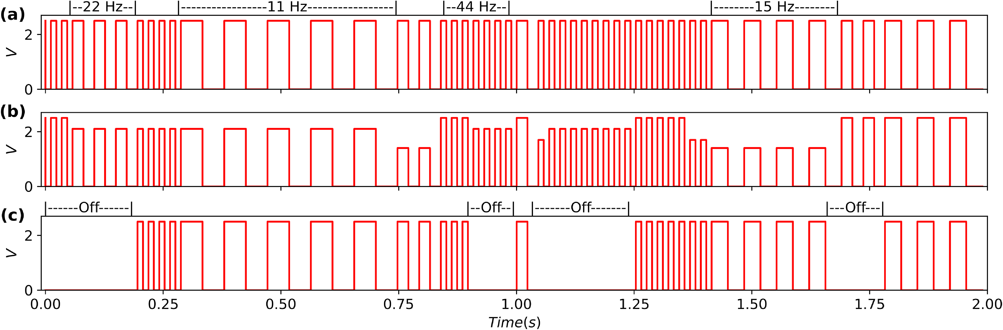
 ϕon=0.5
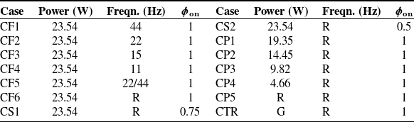
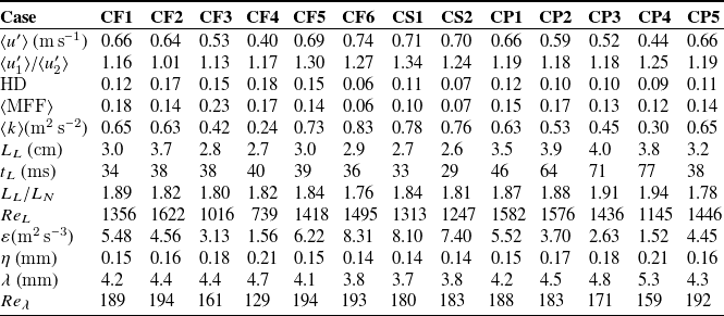
 ⟨⋅⟩


 u1
 u2
 u1
 u2

 u1′
 u2′


 D11(r1)
 x1
 x2
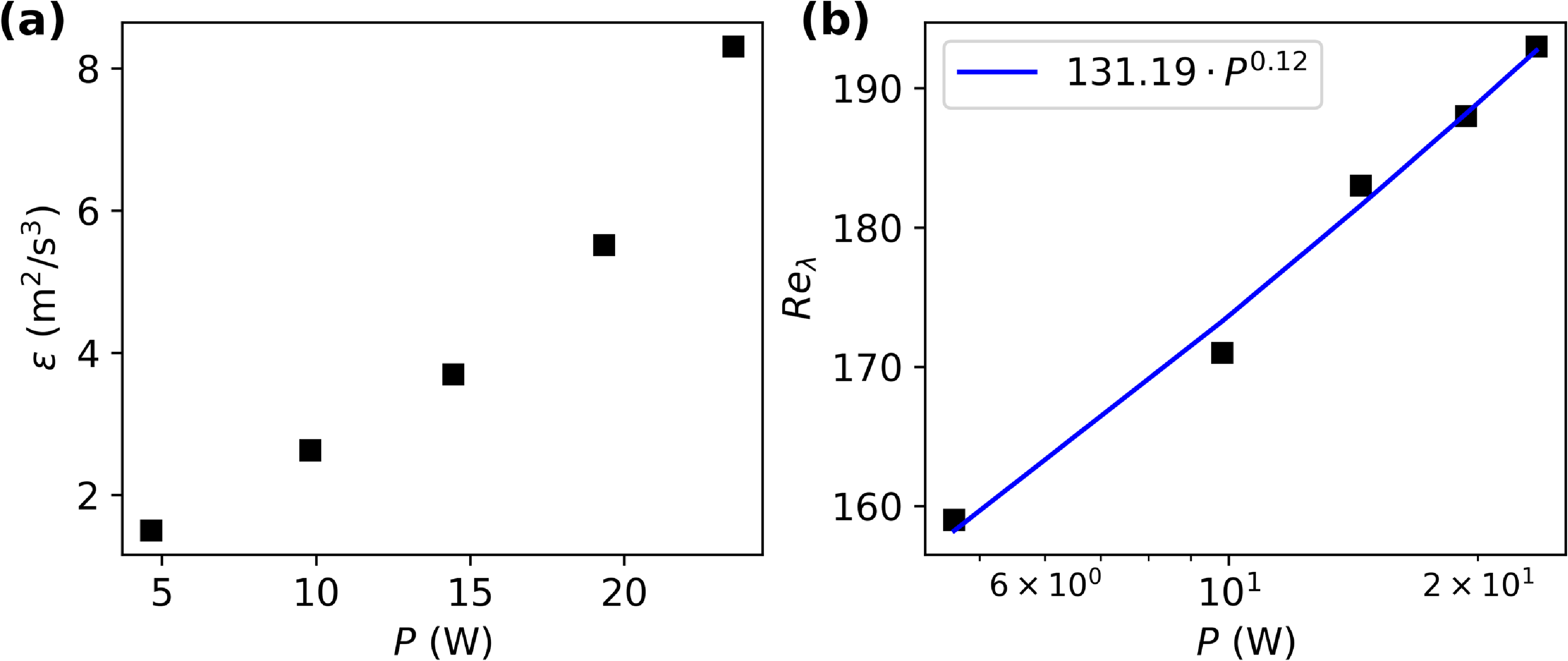
 ε
 Reλ

 Λ[j]/∑j=0NΛ[j]
 ∑j=0nΛ[j]/∑j=0NΛ[j]



 Λ[j]/∑Λ[j]
 R[j]



 Open access

