



1. Introduction
A Gaussian random point set is an independent and identically distributed (i.i.d.) sequence of standard Gaussian random points in
 $\mathbb{R}^d$
, i.e. each point in the set is distributed according to
 $N(0,I_d)$
. The convex hull of a Gaussian random point set
 $\{X_1,\dotsc,X_n\}$
with n samples is denoted by
 $[X_1,\dotsc, X_n]$
and is called a Gaussian random polytope. In the study of random polytopes given as the convex hull of random points, many asymptotic results provide insight in the case where the dimension (d) is fixed but arbitrary and the number of points (n) grows. For example, some of the basic results provide asymptotic expansions on the number of j-dimensional faces of a Gaussian random polytope for fixed d and as
 $n \to \infty$
[Reference Affentranger and Schneider1, Reference Baryshnikov and Vitale4, Reference Hug, Munsonius and Reitzner15, Reference Raynaud24, Reference Rényi and Sulanke25]. For the case where both the dimension and the number of points grow together, there are gaps in our understanding. In this work we study this case. We provide asymptotic expansions of the expectation of several natural quantities associated with Gaussian random polytopes and, more generally, Gaussian random point sets. The quantities we consider are the number of facets, the number of k-facets, and the number of pairs of estranged facets. We now recall the standard definitions of k-facets and estranged facets.
A k-facet of a finite set of points
 $X \subset \mathbb{R}^d$
in general position (namely, any subset of
 $d+1$
or less points is affinely independent) is a subset
 $\Delta \subset X$
of size d such that the open halfspace on one side of
 $\operatorname{aff} \Delta$
contains exactly k points from X. We use the notation
 $E_k(X)$
for the set of k-facets of X and we define
 $e_k(X)\,:\!=|E_k(X)|$
. There is a long line of work on the k-facet problem which requires determination of the asymptotics of the maximum possible number of k-facets of a set of n points in
 $\mathbb{R}^d$
as a function of n, k, and d. The first papers on the k-facet problem ([Reference Erdös, Lovász, Simmons and Straus13] and [Reference Lovász20]) only considered the case when the dimension is equal to two, and even this case is still not well understood. See [Reference Wagner29] for a survey on what is known. Although the majority of work on the k-facet problem is for deterministic point sets, the problem has also previously been studied for random point sets in [Reference Bárány and Steiger2, Reference Clarkson11, Reference Leroux and Rademacher18].
Let P be a full-dimensional polytope. We use the notation
 $f_j(P)$
for the number of j-dimensional faces of P. In particular,
 $f_{d-1}(P)$
is the number of facets. Note that if
 $X \subset \mathbb{R}^d$
is a set of n points in general position, then the 0-facets of X are precisely the facets of the polytope P where P is the convex hull of X, so
 $f_{d-1}(P) = e_0(X)$
in this case.
A pair of facets of a polytope is called estranged if they do not share any vertices (i.e. facets F and G are estranged if the set of vertices contained in F is disjoint from the set of vertices contained in G). Estranged pairs of facets of a polytope also have an interesting interpretation if we take the polar of the original polytope. Since in this discussion we only care about the combinatorics of faces of full-dimensional polytopes, when we say polar we mean the polar with respect to any interior point. In this paper all the polytopes we consider are simplicial with probability 1. The polar of a simplicial polytope is a simple polytope and there is a one-to-one correspondence between pairs of estranged facets of the simplicial polytope P and inner diagonals of the polar
 $P^\ast$
of P. Here, an inner diagonal of a polytope is a line segment which joins two vertices of the polytope and that is contained, except for its endpoints, in the relative interior of the polytope. We clarify the motivation for studying estranged facets and inner diagonals in the next section.
1.1. Previous work and our contributions
1.1.1. Expected number of facets and k-facets.
Let [X] denote the convex hull of X.
As previously mentioned, an asymptotic formula for the expected number of facets of a Gaussian random polytope for fixed dimension as the number of samples n goes to infinity has been known for some time. It was shown in [Reference Raynaud24, Reference Rényi and Sulanke25] that, for fixed
 $d \ge 2$
and a set
 $\{X_1,\dotsc, X_n\}$
of n i.i.d. Gaussian random points in
 $\mathbb{R}^d$
,
 \[ \mathbb{E}f_{d-1} ([X_1, \dotsc, X_n]) = \frac{2^d\pi^{({d-1})/{2}}}{\sqrt{d}}(\ln n)^{({d-1})/{2}}(1+o(1))\]
as
 $n \to \infty$
. Similar formulae are known for
 $\mathbb{E}f_{j} ([X_1, \dotsc, X_n])$
for
 $j=0, \dotsc , d$
[Reference Affentranger and Schneider1, Reference Baryshnikov and Vitale4, Reference Hug, Munsonius and Reitzner15].
The above-mentioned papers only address the case when the dimension is fixed and the number of samples goes to infinity. More recently, progress has been made in [Reference Böröczky, Lugosi and Reitzner7] and in [Reference Fleury14] on the question of the asymptotic value of
 $\mathbb{E}f_{d-1} ([X_1, \dotsc, X_n])$
when both d and n are allowed to go to infinity. It is shown in [Reference Böröczky, Lugosi and Reitzner7, Theorem 1.1] that if
 $d\ge 78$
and
 $n \ge {\mathrm{e}}^{\mathrm{e}} d$
, then
 \begin{align} \mathbb{E}f_{d-1}([X_1,\dotsc,X_n]) & = 2^d\pi^{({d-1})/{2}}d^{-{1}/{2}} \times \exp\bigg\{ \frac{d-1}{2}\operatorname{lln}\frac{n}{d}-\frac{d-1}{4}\frac{\operatorname{lln}({n}/{d})}{\ln({n}/{d})} \nonumber \\ & \quad + (d-1)\frac{\Theta}{\ln({n}/{d})} + O(\sqrt{d}{\mathrm{e}}^{-{d}/{10}})\bigg\}\end{align}
with
 $\Theta \in [{-}34,2]$
and
 $\operatorname{lln}=\log\log$
. Also, [Reference Böröczky, Lugosi and Reitzner7, Theorem 1.3] states that if
 $n-d = o(d)$
, then
 \begin{equation} \mathbb{E}f_{d-1}([X_1,\dotsc,X_n]) = \binom{n}{d}\frac{1}{2^{n-d-1}} \exp\bigg\{\frac{1}{\pi}\frac{(n-d)^2}{d} + O\bigg(\frac{(n-d)^3}{d^2}\bigg) + o(1)\bigg\}.\end{equation}
There are two gaps relevant to us in their expressions: (i) they only provide asymptotic expressions for
 $n-d = o(d)$
or
 $n\geq {\mathrm{e}}^{\mathrm{e}} d$
; (ii) for the case where n grows proportional to d, they only establish exponential upper and lower bounds (with different bases of the exponential function in each bound). Indeed, in the case where
 $n/d \to \alpha >1$
, (1) gives exponential upper and lower bounds for
 $\mathbb{E}f_{d-1} ([X_1, \dotsc, X_n])$
. But because of the parameter
 $\Theta$
, (1) does not determine the constant
 $C(\alpha)$
such that
 $\mathbb{E}f_{d-1} ([X_1, \dotsc, X_n]) = C(\alpha)^{d+o(d)}$
. Our Theorem 2 fills in this missing piece. We show that when
 $n/d \to \alpha > 1$
and
 $k/(n-d) \to r \in [0,1]$
then the expected number of k-facets grows like
 $C(\alpha,r)^{d+o(d)}$
, where
 $C(\alpha,r)$
is a constant depending on
 $\alpha$
and r, and we provide a simple way to determine
 $C(\alpha,r)$
given
 $\alpha$
and r (Theorem 2). Note that setting
 $k=0$
gives the asymptotics of the expected number of facets
 $\mathbb{E}f_{d-1} ([X_1, \dotsc, X_n])$
. We remark that (1) is also valid when
 $n/d \to \infty$
, and that it gives more accurate estimates for
 $\mathbb{E}f_{d-1} ([X_1, \dotsc, X_n])$
when n grows exponentially with d than it does for the case where
 $n/d \to \alpha$
[Reference Böröczky, Lugosi and Reitzner7]. We do not consider the exponential growth case in this work.
The convex hull of random points from the unit sphere in
 $\mathbb{R}^d$
was considered in [Reference Bonnet and O’Reilly6], calling such polytopes spherical random polytopes and providing asymptotic expressions for the expected number of facets as n and d grow at different rates. In the cases when
 $n-d= o(d)$
or
 $n/d \to \infty$
and
 $\log n /d \to 0$
, formulae were obtained for the expected number of facets of spherical random polytopes which match the corresponding formulae obtained in [Reference Böröczky, Lugosi and Reitzner7] for the expected number of facets of Gaussian random polytopes, i.e. (1) and (2). Such a correspondence is not particularly surprising given the fact that Gaussian random points concentrate around a thin spherical shell of radius
 $\sqrt{d}$
in high dimension. Our result shows that this correspondence continues for the case when n is proportional to d: for any
 $\alpha>1$
, Theorem 2 says that the expected number of facets of a Gaussian random polytope with
 $n\sim \alpha d$
vertices is equal to
 $C(\alpha)^{d+o(d)}$
for some constant
 $C(\alpha)$
. For spherical random polytopes, the case when the number of vertices is equal to
 $n\sim \alpha d$
for some
 $\alpha>1$
is dealt with in [Reference Bonnet and O’Reilly6, Theorem 4.2]. The asymptotic formula given there is also of the form
 $C(\alpha)^{d+o(d)}$
for some constant
 $C(\alpha)$
. Some algebra shows that the constants are the same in both the spherical and Gaussian random cases.
1.1.2. A formula from [Reference Hug, Munsonius and Reitzner15] extended to k-facets.
A formula is provided in [Reference Hug, Munsonius and Reitzner15, Theorem 3.2] that expresses the probability that a fixed subset of d out of n Gaussian random points form a facet of the convex hull of the whole set. The formula turns the original probability involving n random vectors in
 $\mathbb{R}^d$
into a simpler probability involving
 $n-d+1$
real-valued random variables. The proof there is an application of the affine Blaschke–Petkantschin formula.
We extend the formula to the case of k-facets (Theorem 1). Our proof does not use the Blaschke–Petkantschin formula and is based on a slightly different probabilistic argument.
1.1.3. Expected number of pairs of estranged facets.
We show in Theorem 3 that if X is a set of 2d i.i.d. Gaussian random points in
 $\mathbb{R}^d$
, then the expected number of pairs of estranged facets of [X] is equal to
 $C^{d+o(d)}$
, where
 $C\approx 1.7696$
.
The main technique in the proof is the affine Blaschke–Petkantschin formula applied twice on a partition of the 2d points into two d-subsets to express the probability that they are facets simultaneously. This is combined with known estimates of the expected volume of a random simplex (one of the main terms in the affine Blaschke–Petkantschin formula) and a simple asymptotic expansion of integrals (Proposition 4).
To put this result in context, we recall the following conjecture.
Conjecture 1. (von Stengel [Reference von Stengel28].) The maximum number of pairs of estranged facets of any simplicial d-polytope with 2d vertices is
 $2^{d-1}$
, which is attained by the d-dimensional cross polytope.
Although von Stengel’s conjecture is still open, a number of similar questions about estranged facets (and their polar equivalent, inner diagonals) were answered in [Reference Bremner and Klee10], which argued that estranged facets are worthy of more study given that they are an intrinsically interesting combinatorial feature of convex polytopes.
Aside from their intrinsic interest, estranged facets are also relevant to the study of Nash equilibria of bimatrix games [Reference von Stengel28]. Indeed, this was the original context for von Stengel’s conjecture. Although estranged facets themselves do not directly correspond to any particular quantity of interest in bimatrix games, they have been used in [Reference Bárány, Vempala and Vetta3] in the analysis of a Las Vegas algorithm for finding Nash equilibria in bimatrix games. In particular, the analysis required the determination of concentration bounds for the number of Nash equilibria in random games. This in turn required proof of an upper bound on the expected number of pairs of estranged facets of a random polytope whose vertices are either i.i.d. Gaussian or uniform in the d-cube [Reference Bárány, Vempala and Vetta3, Lemma 13]. In contrast to our Theorem 3, [Reference Bárány, Vempala and Vetta3, Lemma 13] is only meaningful in the case when the dimension d is fixed and the number of points n goes to infinity.
Finally, we remark that estranged facets are also relevant to the study of the diameter problem for convex polytopes, i.e. the question of the maximum diameter of the graph of a simple d-polytope with n facets. As previously mentioned, estranged facets of a simplicial polytope correspond, via the polar operation, to inner diagonals of a simple polytope. It has been shown that for any n and d such that
 $n\ge 2d$
, the maximum diameter over all simple d-polytopes with n facets is attained by the distance between two vertices which form an inner diagonal of one such polytope [Reference Klee and Walkup17, Theorem 2.8].
1.1.4. Simple asymptotic expansion of integrals.
Our asymptotic expansions of expected values are based on the formula
 $\int_{\mathbb{R}^d} f(x)^p\,\mathrm{d} x = {\lVert f\rVert}_\infty^{p+o(p)}$
, stated formally as Proposition 4. This is a simple result that provides asymptotic expansions of integrals and follows immediately from the known fact that the
 $L^p$
norm of a function converges to the
 $L^\infty$
norm as
 $p \to \infty$
under mild assumptions (Proposition 3). We remark that Proposition 4 is tailored to the specific asymptotic regime that we consider, i.e. when the number of vertices n grows linearly with the dimension d. It is not immediately useful when considering slower or faster regimes.
1.2. Outline of the paper
Section 2 introduces our notation and collects some propositions that will be used later, including a result about the expected volume of a Gaussian simplex as well as a result about asymptotic expansions of integrals based on
 $L^p$
norms. In Section 3 we establish our asymptotic formula for the expected number of k-facets of a Gaussian random polytope. Finally, Section 4 establishes the asymptotic formula for the expected number of estranged facets of a Gaussian random polytope with 2d vertices.
2. Preliminaries
Let
 $f_X$
denote the probability density function (PDF) of random variable X. Let
 $\operatorname{\mathbb{E}}_X(f(X,Y))$
denote the expectation with respect to X only, and similarly for
 $\mathbb{P}_X$
. Namely,
 $\operatorname{\mathbb{E}}_X(f(X,Y)) = \operatorname{\mathbb{E}}(f(X,Y) \mid Y)$
. For a random vector X, let
 $\operatorname{cov}(X)$
denote the covariance matrix of X. The asymptotic notation
 $f(d) \sim g(d)$
means
 $f(d)/g(d) \to 1$
as
 $d \to \infty$
. For a set A in a measurable space, let
 $\operatorname{\mathbf{1}}_{A}$
denote the indicator function of A. For a measurable set
 $K \subseteq \mathbb{R}^d$
, let
 $\lvert K \rvert$
denote the volume of K. Let [X] denote the convex hull of X. Let
 $\omega_d = 2 \pi^{d/2}/\Gamma(d/2)$
be the
 $(d-1)$
-dimensional volume of the unit sphere in
 $\mathbb{R}^d$
. The binary entropy function H is defined on (0,1) by
 $H(p) = -p\log_2(p) -(1-p)\log_2(1-p)$
and
 $H(0) = H(1) = 0$
.
We will need the following characterization of the shortest vector in an affine hull.
Lemma 1. Given linearly independent vectors
 $p_1, p_2, \dotsc, p_d \in \mathbb{R}^d$
, the shortest vector in their affine hull is
 $v = {P^{-1}\mathbf{1}}/{\lVert P^{-1} \mathbf{1}\rVert^2}$
, where
 $P = ( p_1\ \cdots\ p_d )^\top$
. In particular,
 ${\lVert v\rVert}= {1}/{{\lVert P^{-1}\mathbf{1}\rVert}}$
.
Proof. From [Reference Loera, Haddock and Rademacher19, Lemma 1.2], the shortest vector in the affine hull, v, satisfies
 $Pv = {\lVert v\rVert}^2 \mathbf{1}$
. Since P is full rank,
 $v = {\lVert v\rVert}^2 P^{-1} \mathbf{1}$
. Compute norms of the vectors in this equation to get
 ${\lVert v\rVert} = 1/{\lVert P^{-1} \mathbf{1}\rVert}$
. The claim follows.
We will also need the following formula that relates the second moment of the volume of a random simplex with the determinant of the covariance matrix of the underlying distribution.
Proposition 1. (Blaschke’s formula, [Reference Brazitikos, Giannopoulos, Valettas and Vritsiou9, Proposition 3.5.5], [Reference Rademacher23, Lemma 4].) Let
 $X_1,\dotsc,X_{d+1}$
be i.i.d. d-dimensional random vectors with finite second moment. Then
 $\det\operatorname{cov}(X_1) = ({d!}/({d+1}))\operatorname{\mathbb{E}}(\lvert{[X_1,\dotsc,X_{d+1}]}\rvert^2)$
.
Proof. [Reference Rademacher23, Lemma 4] states and proves the claim for the uniform distribution in a convex body. That proof works essentially unchanged for any distribution with finite second moment.
We will need the following well-known result about the expected volume of a Gaussian simplex (see, e.g., [Reference Miles22, p. 377]).
Proposition 2. Let
 $X_1,\dotsc,X_{d+1}$
be i.i.d. d-dimensional Gaussian random vectors. Then
 \[ \operatorname{\mathbb{E}}(\lvert{[X_1,\dotsc,X_{d+1}]}\rvert) = \frac{\sqrt{d+1}}{2^{d/2}\Gamma(({d}/{2})+1)} \sim \frac{1}{\sqrt{\pi}\,}\bigg(\frac{{\mathrm{e}}}{d}\bigg)^{d/2}. \]
We use the following asymptotic approximation of integrals:
 $\int_{\mathbb{R}^d} f(x)^p\,\mathrm{d}x = {\lVert f\rVert}_\infty^{p+o(p)}$
(Proposition 4). It follows easily from the fact that the
 $L^p$
norm converges to the
 $L^\infty$
norm as
 $p \to \infty$
under mild assumptions (Proposition 3).
Proposition 3. ([Reference Rudin26, p. 71].) Let
 $1\leq q < \infty$
. Let
 $f \in L^\infty(\mathbb{R}^d) \cap L^q(\mathbb{R}^d)$
. Then
 ${\lVert f\rVert}_\infty = \lim_{p \to \infty} {\lVert f\rVert}_p$
.
Proposition 4. Let
 $1\leq q < \infty$
. Let
 $f \in L^\infty(\mathbb{R}^d) \cap L^q(\mathbb{R}^d)$
and assume that f is nonnegative and
 $C\,:\!= {\lVert f\rVert}_\infty \neq 1$
. Then, as
 $p \to \infty$
,
 $\int_{\mathbb{R}^d} f(x)^p\,\mathrm{d}x = C^{p+o(p)}$
(where o(p) can depend on f).
Proof. Let
 $a_p = \int_{\mathbb{R}^d} f(x)^p\,\mathrm{d} x$
. From Proposition 3 we have
 $\lim_{p \rightarrow \infty} a_p^{1/p} = C$
. Write
 $a_p = C^{p + g(p)}$
for some function g.
To conclude, we will now show that
 $g(p) = o(p)$
. Note that
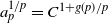 $a_p^{1/p} = C^{1+{g(p)}/{p}}$
, so that, applying
 $\lim_{p \to \infty}$
to both sides,
 $\lim_{p \to \infty} C^{{g(p)}/{p}} = 1$
, which implies
 $\lim_{p \to \infty} ({g(p)}/{p}) = 0$
.
We need the following known inequality (the constant has not been optimized).
Lemma 2. If X is a (real-valued) mean-zero logconcave random variable then
 $\operatorname{\mathbb{E}}(\lvert X\rvert) \geq \frac{1}{8}\sqrt{\operatorname{\mathbb{E}}(X^2)}$
.
Proof. The inequality is invariant under scaling and therefore it is enough to prove it when X is isotropic (i.e. when
 $\operatorname{\mathbb{E}}(X^2)=1$
). It is known [Reference Lovász and Vempala21, Lemma 5.5] that the density of an isotropic logconcave random variable is at most 1. Therefore, using Markov’s inequality,
 $ \frac12 \leq \mathbb{P}\big(\lvert X\rvert \geq \frac14\big) \leq 4\operatorname{\mathbb{E}}(\lvert X\rvert)$
. The claim follows.
3. Facets and k-facets
In this section we study the expected number of k-facets of Gaussian random polytopes. We give an asymptotic formula for the expected number of k-facets in the case when the dimension d goes to infinity and the number of samples n grows linearly with d.
Before establishing our asymptotic formula, we need to establish the following result which reduces the problem of computing
 $\mathbb{E}e_k (\{X_1, \dotsc, X_n\})$
from a d-dimensional problem to a one-dimensional problem.
Theorem 1. Let
 $X_1,\dotsc,X_n$
be
 $n \ge d+1$
i.i.d. standard Gaussian random vectors in
 $\mathbb{R}^d$
. Then the expected number of k-facets of
 $\{X_1,\dotsc,X_n\}$
is equal to
 $\binom{n}{d}\mathbb{P}(Y \in E_k(\{Y,Y_1,\dotsc,Y_{n-d}\}))$
, where Y is
 $N(0,{1}/{d})$
,
 $Y_i$
is
 $N(0, 1)$
for
 $i = 1,\dotsc,n-d$
, and
 $Y,Y_1,\dotsc,Y_{n-d}$
are independent.
Proof. By linearity of expectation and symmetry, it is enough to show that the probability that
 $\{X_1,\dotsc,X_d\}$
is a k-facet is
 $\mathbb{P}(Y \in E_k(\{Y,Y_1,\dotsc,Y_{n-d}\}))$
.
Let V be a random unit vector perpendicular to
 $\operatorname{aff}\{X_1,\dotsc,X_d\}$
but with its orientation (sign) chosen independently at random between the two choices. Define
 $Y = V\cdot X_1$
and
 $Y_i = V \cdot X_{i+d}$
,
 $i=1,\dotsc,n-d$
. Using that V is independent of
 $X_{d+1},\dotsc,X_{n}$
, it is clear that the
 $Y_i$
are i.i.d. N(0,1). Moreover, notice that, by symmetry, the distribution of V conditioned on Y is still uniform on the unit sphere. That is, V is independent of Y, which implies that Y is independent of
 $Y_1,\dotsc,Y_{n-d}$
.
We now determine the distribution of Y. Note that
 $Y^2$
is the squared distance of
 $\operatorname{aff}\{X_1,\dotsc$
,
 $X_d\}$
from the origin. From Lemma 1, the squared distance of
 $\operatorname{aff}\{X_1,\dotsc,X_d\}$
from the origin is given by
 $1/\lVert A^{-1}\mathbf{1}\rVert^2$
, where A is the matrix having
 $X_1,\dotsc,X_d$
as rows. By the invariance under orthogonal transformations of the distribution of A, the distribution of
 $A^{-1}$
is also invariant under orthogonal transformations and the distribution of
 $1/\lVert A^{-1}\mathbf{1}\rVert^2$
is the same as the distribution of
 ${1}/{d\lVert A^{-1}e_1\rVert^2}$
. In this expression,
 ${1}/{\lVert A^{-1}e_1\rVert^2}$
is the squared length of the first column of
 $A^{-1}$
, which is equal to the squared distance between
 $X_1$
and
 $\operatorname{span}\{X_2,\dotsc,X_d\}$
by the definition of inverse matrix. This is distributed as
 $\chi^2_1$
or, in other words, N(0,1) squared. Thus, using the random sign of V, the distribution of Y is
 $N(0,1/d)$
.
In summary, Y and the
 $Y_i$
are distributed as in the statement. Moreover, the event that
 $\{X_1,\dotsc,X_d\}$
is a k-facet of
 $\{X_1,\dotsc,X_n\}$
is the same as the event that Y is a k-facet of
 $ \{Y,Y_1,\dotsc,Y_{n-d}\}$
.
We remark that Theorem 1 is heavily inspired by [Reference Hug, Munsonius and Reitzner15]. In particular, Theorem 1 is a simple generalization of [Reference Hug, Munsonius and Reitzner15, Theorem 3.2] from facets to k-facets. See [Reference Hug, Munsonius and Reitzner15, Theorem 3.2] for an alternative proof of Theorem 1 (in the case of facets) using the affine Blaschke–Petkantschin formula.
We are now ready to state our main result on facets/k-facets of Gaussian random polytopes. We use the notation
 \[ \Phi(y) \,:\!= \frac{1}{\sqrt{2\pi}\,}\int_{-\infty}^y{\mathrm{e}}^{-{s^2}/{2}}\,\mathrm{d}s, \qquad \phi(y) \,:\!= \Phi'(y) = \frac{1}{\sqrt{2\pi}\,}{\mathrm{e}}^{-{y^2}/{2}}\]
for the cumulative distribution function and PDF of the standard Gaussian distribution.
Theorem 2. Fix
 $\alpha>1$
and
 $r \in [0,1]$
, and assume that
 $n/d \to \alpha$
as
 $d \to \infty$
and that
 $k/(n-d) \to r$
as
 $d \to \infty$
. Let X be a set of n i.i.d. Gaussian random points in
 $\mathbb{R}^d$
. Then the expected number of k-facets of X is equal to
 $(2^{\alpha H({1}/{\alpha})}2^{(\alpha-1)H(r)}\sqrt{2\pi}c_{\alpha,r})^{d+o(d)}$
as
 $d\to\infty$
, where
 $c_{\alpha,r} \,:\!= \max_{y\in\mathbb{R}}\{\Phi(y)^{r(\alpha-1)}(1-\Phi(y))^{(1-r)(\alpha-1)}\phi(y)\}$
and H(r) is the binary entropy function. The rate of convergence in the above o(d) is not universal as it depends on
 $\alpha$
and r, and on the rate of convergence of
 $n/d$
to
 $\alpha$
and
 $k/(n-d)$
to r.
Proof. From Theorem 1,
 $\mathbb{E}e_k(X) = \binom{n}{d}\mathbb{P}(Y\in E_k(\{Y,Y_1,\dotsc,Y_{n-d}\}))$
where Y is
 $N(0,{1}/{d})$
,
 $Y_i$
is N(0,1) for
 $i = 1,\dotsc,n-d$
, and
 $Y,Y_1,\dotsc,Y_{n-d}$
are independent. Notice that if
 $k\neq({n-d})/{2}$
, then
 \[ \mathbb{P}(Y\in E_k(\{Y,Y_1,\dotsc,Y_{n-d}\})) = 2\binom{n-d}{k}\frac{\sqrt{d}}{\sqrt{2\pi}\,} \int_{-\infty}^{\infty}\Phi(y)^k(1-\Phi(y))^{n-d-k}{\mathrm{e}}^{-{dy^2}/{2}}\,\mathrm{d}y. \]
If
 $k = ({n-d})/{2}$
, this formula counts each potential k-facet twice, because in this case each side of the hyperplane represented by Y could contain exactly
 $({n-d})/{2}$
points. Therefore, if
 $k = ({n-d})/{2}$
, the formula holds after removing the factor of two on the right-hand side. This factor of two is not important for our result, and we have
 \begin{align*} \mathbb{E}e_k(X) & = \Theta(1)\binom{n}{d}\mathbb{P}(Y\in E_k(\{Y,Y_1,\dotsc,Y_{n-d}\})) \\ & = \Theta(1)\binom{n}{d}\binom{n-d}{k}\frac{\sqrt{d}}{\sqrt{2\pi}\,} \int_{-\infty}^{\infty}\Phi(y)^k(1-\Phi(y))^{n-d-k}{\mathrm{e}}^{-{dy^2}/{2}}\,\mathrm{d}y \\ & = \Theta(1)\binom{n}{d}\binom{n-d}{k}\sqrt{d}(2\pi)^{({d-1})/{2}} \int_{-\infty}^{\infty}\Phi(y)^k(1-\Phi(y))^{n-d-k}\phi(y)^d\,\mathrm{d}y. \end{align*}
We will use Proposition 4 to estimate the integral in this expression. In particular, we will show that the integral is equal to
 $c_{\alpha,r}^{d+o(d)}$
, where
 $c_{\alpha,r}\,:\!=\|f\|_\infty$
and
 $f(y) \,:\!= \Phi(y)^{r(\alpha-1)}(1-\Phi(y))^{(1-r)(\alpha-1)}\phi(y)$
. In order to establish this estimate, we first need to restrict the integral to some finite interval, the length of which does not depend on d but does depend on
 $\alpha,r$
. In order to accomplish this, first observe that we can upper bound the terms in front of the integral by
 $\binom{n}{d}\binom{n-d}{k}\sqrt{d}(2\pi)^{({d-1})/{2}} = O(2^n2^n(2\pi)^{({d-1})/{2}}) = O((4^{\alpha}\sqrt{2\pi})^d)$
. Now choose
 $R(\alpha)$
so that
 $\phi(R(\alpha)) < {1}/{4^\alpha\sqrt{2\pi}}$
. For technical reasons, we also need to assume that our region of integration is big enough so that it contains some
 $y_0 \in \mathbb{R}$
such that
 $c_{\alpha,r} = f(y_0)$
. So choose
 $R(\alpha,r)$
such that
 $R(\alpha,r)\ge R(\alpha)$
and so that
 $[{-}R(\alpha,r),R(\alpha,r)]$
contains
 $y_0$
as above. Using the fact that
 $\Phi(y)^k(1-\Phi(y))^{n-d-k}<1$
and
 $\phi(R(\alpha,r))<{1}/{4^\alpha\sqrt{2\pi}}$
, we know that the right tail of the integral is upper bounded by
 \begin{align*} \int_{R(\alpha,r)}^{\infty}\Phi(y)^k(1-\Phi(y))^{n-d-k}\phi(y)^d\,\mathrm{d}y & \le \int_{R(\alpha,r)}^{\infty}\phi(y)^{d-1}\phi(y)\,\mathrm{d}y \\ & \le \bigg(\frac{1}{4^\alpha\sqrt{2\pi}}\bigg)^{d-1}\int_{R(\alpha,r)}^{\infty}\phi(y)\,\mathrm{d}y = O((4^\alpha\sqrt{2\pi})^{-d}), \end{align*}
and the same estimate holds for the left tail. Therefore,
 \begin{align*} \mathbb{E}e_k(X) & = \Theta(1)\binom{n}{d}\binom{n-d}{k}\sqrt{d}(2\pi)^{({d-1})/{2}} \int_{-\infty}^{\infty}\Phi(y)^k(1-\Phi(y))^{n-d-k}\phi(y)^d\,\mathrm{d}y \\ & = \Theta(1)\binom{n}{d}\binom{n-d}{k}\sqrt{d}(2\pi)^{({d-1})/{2}} \int_{-R(\alpha,r)}^{R(\alpha,r)}\Phi(y)^k(1-\Phi(y))^{n-d-k}\phi(y)^d\,\mathrm{d}y + O(1) \\ & = \Theta(1)\binom{n}{d}\binom{n-d}{k}\sqrt{d}(2\pi)^{({d-1})/{2}} \int_{-R(\alpha,r)}^{R(\alpha,r)}\Phi(y)^k(1-\Phi(y))^{n-d-k}\phi(y)^d\,\mathrm{d}y, \end{align*}
where the last equality uses the fact that
 $\mathbb{E}e_k(X)\ge1$
so that the O(1) term can be absorbed into the
 $\Theta(1)$
factor in front.
Now, for
 $y \in [{-}R(\alpha,r),R(\alpha,r)]$
,
 $\Phi(y)$
and
 $1-\Phi(y)$
both take values in some fixed interval, i.e.
 $\Phi(y) = \Theta(1)$
and
 $1-\Phi(y) = \Theta(1)$
. Recall that we are assuming that
 $n/d \to \alpha$
and
 $k/(n-d)\to r$
as
 $d \to \infty$
, which means that
 $n = \alpha d + o(d)$
and
 $k = r(\alpha-1)d+o(d)$
, and therefore that
 $n-d-k = (\alpha-1)d-r(\alpha-1)d+o(d)$
. This means that
 $\Phi(y)^k = \Phi(y)^{r(\alpha-1)d}\Theta(1)^{o(d)} = {\mathrm{e}}^{o(d)}\Phi(y)^{r(\alpha-1)d}$
, and that
 $(1-\Phi(y))^{n-d-k} = (1-\Phi(y))^{(\alpha-1)d-r(\alpha-1)d}\Theta(1)^{o(d)} = {\mathrm{e}}^{o(d)}(1-\Phi(y))^{(\alpha-1)d-r(\alpha-1)d}$
for
 $y \in [{-}R(\alpha,r),R(\alpha,r)]$
. Therefore, we have shown that
 \begin{multline*} \int_{-R(\alpha,r)}^{R(\alpha,r)}\Phi(y)^k(1-\Phi(y))^{n-d-k}\phi(y)^d\,\mathrm{d}y \\ = {\mathrm{e}}^{o(d)}\int_{-R(\alpha,r)}^{R(\alpha,r)}\Phi(y)^{r(\alpha-1)d}(1-\Phi(y))^{(1-r)(\alpha-1 )d}\phi(y)^d\,\mathrm{d}y. \end{multline*}
Let
 $\hat{f}\,:\!=f\cdot\operatorname{\mathbf{1}}_{-R(\alpha,r) < y < R(\alpha,r)}$
. Define
 $\hat{c}_{\alpha,r} \,:\!= \|\hat{f}\|_{\infty}$
. Recall that we are assuming that f attains its maximum somewhere in the interval
 $[{-}R(\alpha,r),R(\alpha,r)]$
, so
 $\hat{c}_{\alpha,r} = c_{\alpha,r}$
.
By Proposition 4,
 \[ \int_{-R(\alpha,r)}^{R(\alpha,r)}\Phi(y)^{r(\alpha-1)d}(1-\Phi(y))^{(1-r)(\alpha-1)d}\phi(y)^d\,\mathrm{d}y = (\hat{c}_{\alpha,r})^{d+o(d)} = (c_{\alpha,r})^{d+o(d)}. \]
Combining everything,
 \begin{align*} \mathbb{E}e_k(X) & = \Theta(1)\binom{n}{d}\binom{n-d}{k}\sqrt{d}(2\pi)^{({d-1})/{2}} \int_{-R(\alpha,r)}^{R(\alpha,r)}\Phi(y)^k(1-\Phi(y))^{n-d-k}\phi(y)^d\,\mathrm{d}y \\ & = \Theta(1)\binom{n}{d}\binom{n-d}{k}\sqrt{d}(2\pi)^{({d-1})/{2}}{\mathrm{e}}^{o(d)}(c_{\alpha,r})^{d+o(d)} \\ & = (2^{\alpha H({1}/{\alpha})}2^{(\alpha-1)H(r)}\sqrt{2\pi}c_{\alpha,r})^{d+o(d)}. \end{align*}
In order to obtain the asymptotic estimates of the binomial coefficients as above, we can use the fact that
 $({1}/({n+1}))2^{nH({d}/{n})}\le \binom{n}{d} \le 2^{nH({d}/{n})}$
, which follows from Stirling’s approximation [Reference Cover and Thomas12, Example 11.1.3]. This, combined with the fact that
 $d/n\to1/\alpha$
and that the binary entropy function H is continuous can be used to show that
 $\binom{n}{d} = 2^{\alpha dH({1}/{\alpha})+o(d)}$
. A similar argument applies to the asymptotic estimate of
 $\binom{n-d}{k}$
.
4. Estranged facets
We say that two facets of a polytope are estranged if they do not share any vertices. The main result of this section is the following theorem, which gives an asymptotic estimate of the expected number of estranged facets of the convex hull of 2d Gaussian random points in
 $\mathbb{R}^d$
.
Theorem 3. Let X be a set of 2d i.i.d. Gaussian random points in
 $\mathbb{R}^d$
. Let N be the number of (unordered) pairs of estranged facets in [X]. Then
 $\operatorname{\mathbb{E}}(N) = (4C_4)^{d+o(d)}$
, where
 $C_4\in\big(0,\frac12\big)$
is the universal constant from Lemma 4.
Our proof uses the affine Blaschke–Petkantschin formula ((5), see also [Reference Schneider and Weil27, Theorem 7.2.7]), a change of variable formula that involves the volume of a random simplex. We will need the following estimate of the volume of a random simplex in a halfspace.
Lemma 3. Let
 $H \subseteq \mathbb{R}^{d-1}$
be a halfspace that contains the origin. Let
 $Z_1,\dotsc,Z_d$
be i.i.d. random vectors, each distributed as standard Gaussian truncated to be in H. Then
 \[ \operatorname{\mathbb{E}}(\lvert{[Z_1,\dotsc,Z_d]}\rvert) \geq \sqrt{1-\frac{2}{\pi}}\frac{\sqrt{d}}{2^{({d+5})/{2}}\Gamma(({d+1})/{2})} = \bigg(\frac{{\mathrm{e}}}{d}\bigg)^{d/2}2^{o(d)} \]
(where o(d) does not depend on H).
Proof. Let Z denote the
 $(d-1)\times d$
matrix with columns
 $Z_1,\dotsc,Z_d$
. The idea of the proof is to compare Z with the Gaussian case (namely, without truncation). It is easier to do this for the second moment instead of the first, and we can relate the first and the second moments via Jensen’s inequality and a suitable reverse for our case, Lemma 2.
By applying a rotation, it is enough to prove the statement for
 $H = \{x \in \mathbb{R}^{d-1} \colon x_1 \leq t\}$
with
 $t\geq 0$
. Let W be Z with a row of ones appended. Then
 \begin{equation} \lvert[Z_1, \ldots, Z_d] \rvert/d = \lvert\det(W)\rvert/d!. \end{equation}
That is,
 $\lvert[Z_1,\ldots,Z_d]\rvert = \lvert\det(W)\rvert/(d-1)!$
. Let
 $W_1,\dotsc,W_d$
be the rows of W. Let
 $A = \{x\in\mathbb{R}^d\colon \text{for all } i,\, x_i \leq t \}$
. Note that
 $W_1$
is distributed as standard Gaussian truncated to A. We have
 $\lvert\det(W)\rvert = \prod_{i=1}^d \operatorname{d}(W_i, \operatorname{span} W_{(i+1)\ldots d})$
(where
 $\operatorname{d}(\cdot,\cdot)$
denotes point-subspace distance and
 $W_{a\dotsc b}$
is shorthand notation for
 $W_a,\dotsc,W_b$
) and
 \begin{align} \operatorname{\mathbb{E}}(\lvert\det(W)\rvert) & = \operatorname{\mathbb{E}}\Bigg(\operatorname{d}(W_1,\operatorname{span}W_{2\ldots d}) \prod_{i=2}^d\operatorname{d}(W_i,\operatorname{span}W_{(i+1)\ldots d})\Bigg) \\ & = \operatorname{\mathbb{E}}\Bigg( \operatorname{\mathbb{E}}(\operatorname{d}(W_1,\operatorname{span}W_{2\ldots d}) \mid W_{2\ldots d}\bigr) \prod_{i=2}^d\operatorname{d}(W_i,\operatorname{span}W_{(i+1)\ldots d})\Bigg). \nonumber \end{align}
Let
 $v \in \mathbb{R}^d$
be such that
 $\sum_{i=1}^d v_i = 0$
and
 ${\lVert v\rVert} = 1$
. Using Lemma 2,
 $\operatorname{\mathbb{E}}(v^\top W_1) = 0$
, and the fact that the variance of a Gaussian truncated to
 $({-}\infty, t]$
with
 $t\geq 0$
is at least
 $1- 2/\pi$
, we get
 \begin{equation*} \operatorname{\mathbb{E}}(\lvert v^\top W_1\rvert) \geq \frac{1}{8}\sqrt{\operatorname{\mathbb{E}}((v^\top W_1)^2)} = \frac{1}{8}\sqrt{\text{var}(v^\top W_1)} \geq \frac{1}{8}\sqrt{1-\frac{2}{\pi}} \,:\!= c'. \end{equation*}
Now, to express
 $ \operatorname{d}(W_1,\operatorname{span}W_{2\ldots d})$
, let V be a random vector that is a unit vector normal to
 $\operatorname{span}W_{2\ldots d}$
(sign will not matter) and let
 $W_1'$
be an independent standard Gaussian in
 $\mathbb{R}^d$
. We have the following comparison inequality between
 $W_1$
(truncated Gaussian) and
 $W_1'$
(not truncated), using moment inequalities and the fact that, conditioning on
 $W_{2\ldots d}$
, vector V is a fixed unit vector perpendicular to the all-ones vector
 $W_d$
so that our analysis for v above applies:
 \begin{align*} \operatorname{\mathbb{E}}(\operatorname{d}(W_1,\operatorname{span}W_{2\ldots d}) \mid W_{2\ldots d}) = \operatorname{\mathbb{E}}(\lvert V^\top W_1\rvert \mid W_{2\ldots d}) & \geq c' \\ & = c'\sqrt{\operatorname{\mathbb{E}}(\operatorname{d}(W_1',\operatorname{span}W_{2\ldots d})^2 \mid W_{2\ldots d})} \\ & \geq c'\operatorname{\mathbb{E}}(\operatorname{d}(W_1',\operatorname{span}W_{2\ldots d}) \mid W_{2\ldots d}). \end{align*}
This, in (4), implies, defining W
′ as W with the first row
 $W_1$
substituted by
 $W_1'$
,
 \begin{align*} \operatorname{\mathbb{E}}(\lvert\det(W)\rvert) & \geq c'\operatorname{\mathbb{E}}\Bigg( \operatorname{\mathbb{E}}(\operatorname{d}(W_1',\operatorname{span}W_{2\ldots d}) \mid W_{2\ldots d}) \prod_{i=2}^d\operatorname{d}(W_i,\operatorname{span}W_{(i+1)\ldots d})\Bigg) \\ & = c'\operatorname{\mathbb{E}}\Bigg(\operatorname{d}(W_1',\operatorname{span}W_{2\ldots d}) \prod_{i=2}^d\operatorname{d}(W_i,\operatorname{span}W_{(i+1)\ldots d})\Bigg) \\ & = c'\operatorname{\mathbb{E}}(\lvert\det(W')\rvert) \\ & = c'\frac{(d-1)!\sqrt{d}}{2^{({d-1})/{2}}\Gamma(({d+1})/{2})} \quad \text{(using Proposition 2 and the idea in (3))}. \end{align*}
Thus,
 \begin{equation*} \operatorname{\mathbb{E}}(\lvert[Z_1,\ldots,Z_d]\rvert) = \frac{\operatorname{\mathbb{E}}(\lvert\det(W)\rvert)}{(d-1)!} \geq \frac{c'\sqrt{d}}{2^{({d-1})/{2}}\Gamma(({d+1})/{2})}. \end{equation*}
We now complete the proof of Theorem 3. Most of the proof is in Lemma 4, which estimates the probability that a fixed partition of the random points is a pair of facets. Theorem 3 then follows by linearity of expectation. The proof of Lemma 4 is somewhat similar to the proof of [Reference Hug and Reitzner16, Theorem 1.3], which gives an upper bound for the variance of the number of facets of a Gaussian random polytope in the case where the dimension is fixed and the number of points increases. The main difficulty in the proof of both [Reference Hug and Reitzner16, Theorem 1.3] and Lemma 4 is to prove an upper bound on the probability that a partition of the vertices forms two facets. In contrast to [Reference Hug and Reitzner16, Theorem 1.3], our Lemma 4 is meaningful when the dimension increases with the number of points. However, Lemma 4 does not give any bound on the variance because we only consider pairs of facets with no points in common.
Let F(P) be the set of facets (as a family of subsets of vertices) of polytope P.
Lemma 4. Let X,Y be two independent sequences of d i.i.d. Gaussian random points in
 $\mathbb{R}^d$
. Then
 $\mathbb{P}(X,Y\in F([X,Y])) = C_4^{d+o(d)}$
, where
 \[ C_4 \,:\!= \sup\limits_{\substack{\rho\geq0\\w\in[{-}1,1]}}{\mathrm{e}}^{-\rho^2} \Phi\bigg(\frac{\rho(1-w)}{\sqrt{1-w^2}\,}\bigg)^2\sqrt{1-w^2} \approx 0.4424. \]
Proof. For
 $\theta \in S^{d-1}$
and
 $\rho \in \mathbb{R}_+$
, let
 $H(\rho,\theta) = \{x\in\mathbb{R}^d\colon\theta\cdot x = \rho\}$
,
 $H_-(\rho,\theta) = \{x\in\mathbb{R}^d\colon\theta\cdot x < \rho\}$
, and
 $H_+(\rho,\theta) = \{x\in\mathbb{R}^d\colon\theta\cdot x > \rho\}$
. Let f denote the probability density function of the standard d-dimensional Gaussian distribution.
We will use the following form of the affine Blaschke–Petkantschin formula (as stated in [Reference Hug and Reitzner16, p. 302]; see also [Reference Schneider and Weil27, Theorem 7.2.7]):
 \begin{multline} \int_{\mathbb{R}^d}\dotsi\int_{\mathbb{R}^d}f(x_1,\dotsc,x_d)\,\mathrm{d}x_1\dotsm\,\mathrm{d}x_d \\ = \Gamma(d)\int_{\mathbb{R}_+}\int_{S^{d-1}}\int_{H(\rho,\theta)}\dotsi\int_{H(\rho,\theta)}f(x_1,\dotsc,x_d) \big\lvert\big[{\{x_i\}_{i=1}^d}\big]\big\rvert\, \mathrm{d}x_1\dotsm\,\mathrm{d}x_d\,\mathrm{d}\theta\,\mathrm{d}\rho, \end{multline}
where we use the normalization
 $\int_{S^{d-1}}\mathrm{d}\theta = \omega_d$
, and an integral over an affine hyperplane
 $H(\rho,\theta)\subseteq\mathbb{R}^d$
uses the
 $(d-1)$
-dimensional Lebesgue measure.
We have, using the Blaschke–Petkantschin formula (5) twice:
 \begin{align*} & \mathbb{P}(X,Y\in F([X,Y])) \\ & = \int_{\mathbb{R}^{d^2}}\int_{\mathbb{R}^{d^2}} \operatorname{\mathbf{1}}_{\{x_i\}_{i=1}^d, \{y_i\}_{i=1}^d\in F\left(\left[\{x_i, y_i\}_{i=1}^d\right]\right)} \prod_{i=1}^d f(x_i)\,\mathrm{d}x_i\prod_{i=1}^d f(y_i)\,\mathrm{d}y_i \\ & = \Gamma(d)^2\int_{\mathbb{R}_+^2}\int_{{(S^{d-1})}^2}\int_{{H(\rho_1,\theta_1)}^d}\int_{H(\rho_2,\theta_2)^d} \operatorname{\mathbf{1}}_{\{x_i\}_{i=1}^d \in F\left(\left[\{x_i, y_i\}_{i=1}^d\right]\right)} \operatorname{\mathbf{1}}_{\{y_i\}_{i=1}^d \in F\left(\left[\{x_i, y_i\}_{i=1}^d\right]\right)} \\ & \qquad\qquad\quad \times \big\lvert{\big[\{x_i\}_{i=1}^d\big]}\big\rvert \cdot \big\lvert{\big[\{y_i\}_{i=1}^d\big]}\big\rvert \Bigg(\prod_{i=1}^d f(x_i)\,\mathrm{d}x_i\Bigg)\Bigg(\prod_{i=1}^d f(y_i)\,\mathrm{d}y_i\Bigg)\, \mathrm{d}\theta_1\,\mathrm{d}\theta_2\,\mathrm{d}\rho_1\,\mathrm{d}\rho_2. \end{align*}
Reordering terms,
 \begin{align} & \mathbb{P}(X,Y\in F([X,Y])) \nonumber \\ & = \Gamma(d)^2\int_{\mathbb{R}_+^2}\int_{{(S^{d-1})}^2}\biggl(\int_{{H(\rho_1,\theta_1)}^d} \bigl(\operatorname{\mathbf{1}}_{\{\text{for all }i,\,x_i\in H_+(\rho_2,\theta_2)\}} + \operatorname{\mathbf{1}}_{\{\text{for all }i,\,x_i\in H_-(\rho_2,\theta_2)\}}\bigr) \big\lvert{\big[\{x_i\}_{i=1}^d\big]}\big\rvert \nonumber \\ & \qquad\qquad\qquad\qquad\qquad\qquad\quad \prod_{i=1}^d f(x_i)\,\mathrm{d}x_i\biggr) \nonumber \\ & \qquad\qquad\qquad\qquad \times \biggl(\int_{{H(\rho_2,\theta_2)}^d} \bigl(\operatorname{\mathbf{1}}_{\{\text{for all }i,\,y_i\in H_+(\rho_1,\theta_1)\}} + \operatorname{\mathbf{1}}_{\{\text{for all }i,\,y_i\in H_-(\rho_1,\theta_1)\}}\bigr) \big\lvert{\big[\{y_i\}_{i=1}^d\big]}\big\rvert \nonumber \\ & \qquad\qquad\qquad\qquad\qquad\qquad\quad \prod_{i=1}^d f(y_i)\,\mathrm{d}y_i\biggr)\, \mathrm{d}\theta_1\,\mathrm{d}\theta_2\,\mathrm{d}\rho_1\,\mathrm{d}\rho_2. \end{align}
Upper bound. For the upper bound we continue from (6) by rewriting it as a sum over four cases. The four cases correspond to whether X is on the origin side of
 $\operatorname{aff}Y$
or not, and whether Y is on the origin side of
 $\operatorname{aff}X$
or not:
 \begin{align} & \mathbb{P}(X,Y\in F([X,Y])) \nonumber \\ & = \Gamma(d)^2\sum_{s,s'\in\{-,+\}}\int_{\mathbb{R}_+^2}\int_{{(S^{d-1})}^2}\biggl(\int_{{H(\rho_1,\theta_1)}^d} \operatorname{\mathbf{1}}_{\{\text{for all }i,\,x_i\in H_{s}(\rho_2,\theta_2)\}} \big\lvert{\big[\{x_i\}_{i=1}^d\big]}\big\rvert\prod_{i=1}^df(x_i)\,\mathrm{d}x_i\biggr) \nonumber \\ & \qquad\qquad\qquad\qquad\qquad\qquad \times \biggl(\int_{{H(\rho_2,\theta_2)}^d} \operatorname{\mathbf{1}}_{\{\text{for all }i,\,y_i\in H_{s'}(\rho_1,\theta_1)\}} \big\lvert{\big[\{y_i\}_{i=1}^d\big]}\big\rvert\prod_{i=1}^d f(y_i)\,\mathrm{d}y_i\biggr) \nonumber \\ & \qquad\qquad\qquad\qquad\qquad\qquad \mathrm{d}\theta_1\,\mathrm{d}\theta_2\,\mathrm{d}\rho_1\, \mathrm{d}\rho_2. \end{align}
The next step is to see that each innermost integral in (7) can be interpreted as the expected volume of a random simplex with each vertex according to the Gaussian distribution truncated to a halfspace in
 $\mathbb{R}^{d-1}$
(this is up to a normalization constant to turn the integral into an expectation and after identifying
 $H(\rho_1,\theta_1)$
with
 $\mathbb{R}^{d-1}$
). An upper bound to that expectation will follow immediately from the Brascamp–Lieb inequality. The following notation will be convenient. Let
 $Z=(Z_1,\dotsc,Z_d)\in\mathbb{R}^{(d-1)\times d}$
be i.i.d. standard Gaussian. For the identification of
 $H(\rho_1,\theta_1)$
with
 $\mathbb{R}^{d-1}$
, fix
 $\rho_1,\theta_1$
, and pick an isometry from
 $H(\rho_1,\theta_1)$
to
 $\mathbb{R}^{d-1}$
that maps the minimum Euclidean norm point to the origin. Also let
 $h_s(\rho_1,\theta_1,\rho_2,\theta_2) \subseteq \mathbb{R}^{d-1}$
for
 $s \in \{+,-\}$
denote the image of the halfspace
 $H_s(\rho_2,\theta_2) \cap H(\rho_1,\theta_1)$
in
 $\mathbb{R}^{d-1}$
via the isometry (see Figure 1). Finally, E is the event
 $\{Z\in h_-(\rho_1,\theta_1,\rho_2,\theta_2)^d\}$
, and
 $\mu$
is the standard Gaussian probability measure in
 $\mathbb{R}^{d-1}$
.
Halfspaces in the proof of Lemma 4.

We have
 \begin{multline} \int_{{H(\rho_1,\theta_1)}^d}\operatorname{\mathbf{1}}_{\{\text{for all }i,\,x_i\in H_-(\rho_2,\theta_2)\}} \big\lvert{\big[\{x_i\}_{i=1}^d\big]}\big\rvert\prod_{i=1}^d f(x_i)\,\mathrm{d}x_i \\ = \Bigg(\int_{{H(\rho_1,\theta_1)}^d}\prod_{i=1}^d f(x_i)\,\mathrm{d}x_i\Bigg) \operatorname{\mathbb{E}}_Z(\lvert[Z_1,\ldots,Z_d]\rvert\operatorname{\mathbf{1}}_{E}), \end{multline}
where
 \begin{equation} \int_{{H(\rho_1,\theta_1)}^d}\prod_{i=1}^d f(x_i)\,\mathrm{d}x_i = \frac{{\mathrm{e}}^{-d\rho_1^2/2}}{(2\pi)^{d/2}} \end{equation}
and
 \begin{align} \operatorname{\mathbb{E}}_Z(\lvert[Z_1,\ldots,Z_d]\rvert\operatorname{\mathbf{1}}_{E}) & = \mathbb{P}_Z(E)\operatorname{\mathbb{E}}_Z(\lvert[Z_1,\ldots,Z_d]\rvert \mid E) \nonumber \\ & = (\mu(h_-(\rho_1,\theta_1,\rho_2,\theta_2)))^d \operatorname{\mathbb{E}}_Z(\lvert[Z_1,\ldots,Z_d]\rvert \mid E). \end{align}
We now find an upper bound on the last factor in (10). Let A be the covariance matrix of the Gaussian distribution in
 $\mathbb{R}^{d-1}$
truncated to
 $h_-(\rho_1,\theta_1,\rho_2,\theta_2)$
. Namely,
 $A = \operatorname{cov}(Z_1 \mid Z_1 \in h_-(\rho_1,\theta_1,\rho_2,\theta_2))$
. Note that the variance of any univariate marginal of
 $Z_1$
conditioned on
 $Z_1 \in h_-(\rho_1,\theta_1,\rho_2,\theta_2)$
is at most 1 (say, by the Brascamp–Lieb inequality [Reference Brascamp and Lieb8, Section 5]) and this implies that
 $\det A \leq 1$
. Using moment inequalities and Proposition 1 (Blaschke’s formula),
 \begin{equation} \operatorname{\mathbb{E}}_Z(\lvert[Z_1,\ldots,Z_d]\rvert \mid E) \leq \sqrt{\operatorname{\mathbb{E}}_Z(\lvert[Z_1,\ldots,Z_d]\rvert^2 \mid E)} = \sqrt{\frac{d}{(d-1)!}\det A} \leq \sqrt{\frac{d}{(d-1)!}}. \end{equation}
To complete our understanding of (10), we want to express the Gaussian measure of halfspace
 $h_-(\rho_1,\theta_1,\rho_2,\theta_2)$
in a more explicit way. It will be convenient to understand the signed distance of its boundary to the origin of
 $\mathbb{R}^{d-1}$
. For a halfspace H we define the signed distance to be
 $\operatorname{d}(0,\operatorname{bdry}H)$
if
 $0 \in H$
and
 ${-}\text{d}(0,\operatorname{bdry}H)$
otherwise. Let
 $t(\rho_1,\theta_1,\rho_2,\theta_2)$
denote the signed distance of
 $\operatorname{bdry}h_-(\rho_1,\theta_1,\rho_2,\theta_2)$
to the origin.
We now claim that
 $t(\rho_1,\theta_1,\rho_2,\theta_2) = ({\rho_2-\rho_1\cos\alpha})/{\sin\alpha}$
, where
 $\alpha\in[0,\pi]$
is the angle between
 $\theta_1$
and
 $\theta_2$
. See Figure1 for an illustration of the halfspaces. To see the claim, note first that it is enough to perform this calculation in
 $\mathbb{R}^2$
. Assume without loss of generality that
 $\theta_1=(1,0)$
and
 $\theta_2= (\!\cos\alpha,\sin\alpha)$
. Then
 $t(\rho_1,\theta_1,\rho_2,\theta_2)$
is the y-coordinate of the intersection point of the lines defined by the equations
 $(x,y)\cdot\theta_1 = \rho_1$
and
 $(x,y)\cdot\theta_2 = \rho_2$
, which implies that
 $x=\rho_1$
and
 $\rho_1\cos\alpha + y\sin\alpha = \rho_2$
. The claim follows.
In other words,
 $$ t(\rho_1,\theta_1,\rho_2,\theta_2) = \frac{\rho_2-\rho_1\theta_1\cdot\theta_2}{\sqrt{1-(\theta_1\cdot\theta_2)^2}}. $$
To understand this quantity, it will be helpful in the next calculation to reinterpret certain integrals as expectations and to think of
 $\theta_1$
and
 $\theta_2$
as random unit vectors. With that interpretation, we will use the following known fact: the distribution of the random variable
 $W \,:\!= \theta_1\cdot\theta_2$
has density function
 $$w \mapsto \frac{\Gamma({d}/{2})}{\sqrt{\pi}\Gamma(({d-1})/{2})}(1-w^2)^{({d-3})/{2}}$$
with support
 $[{-}1,1]$
. This follows immediately by symmetry from the fact that any one-dimensional marginal of the uniform distribution in
 $S^{d-1}$
has that density function. See [Reference Bonnet, Grote, Temesvari, Thäle, Turchi and Wespi5, Lemma 6] for a proof of this last fact.
We combine the previous calculations to determine the asymptotics of the first term (
 $s=s'=-$
) in the sum in (7). We start by using (8)– (11),
 \begin{align} & \Gamma(d)^2\int_{\mathbb{R}_+^2}\int_{{(S^{d-1})}^2} \biggl(\int_{{H(\rho_1,\theta_1)}^d}\operatorname{\mathbf{1}}_{\{\text{for all }i,\,x_i\in H_-(\rho_2,\theta_2)\}} \big\lvert{\big[\{x_i\}_{i=1}^d\big]}\big\rvert\prod_{i=1}^d f(x_i)\,\mathrm{d}x_i\biggr) \nonumber \\ & \qquad\qquad\qquad\quad \times \biggl(\int_{{H(\rho_2,\theta_2)}^d} \operatorname{\mathbf{1}}_{\{\text{for all }i,\,y_i\in H_-(\rho_1,\theta_1)\}} \big\lvert{\big[\{y_i\}_{i=1}^d\big]}\big\rvert\prod_{i=1}^d f(y_i)\,\mathrm{d}y_i\biggr) \nonumber \\ & \qquad\qquad\qquad\quad \mathrm{d}\theta_1\,\mathrm{d}\theta_2\,\mathrm{d}\rho_1\,\mathrm{d}\rho_2 \nonumber \\ & \leq \frac{\Gamma(d)^2 d}{(d-1)!(2\pi)^d}\int_{\mathbb{R}_+^2}\int_{{(S^{d-1})}^2} {\mathrm{e}}^{-{d(\rho_1^2+\rho_2^2)}/{2}}(\mu(h_-(\rho_1,\theta_1,\rho_2,\theta_2)))^d (\mu(h_-(\rho_2,\theta_2,\rho_1,\theta_1)))^d \nonumber \\ & \qquad\qquad\qquad\qquad\qquad\qquad \mathrm{d}\theta_1\,\mathrm{d}\theta_2\,\mathrm{d}\rho_1\,\mathrm{d}\rho_2, \end{align}
and in the last expression rewrite the integrals over
 $\theta_1$
and
 $\theta_2$
as expectations and use our earlier calculations about the Gaussian measure of
 $h_-(\cdot)$
to write it as
 \begin{align} & \frac{d!\omega_d^2}{(2\pi)^d}\int_{\mathbb{R}_+^2}{\mathrm{e}}^{-{d\left(\rho_1^2+\rho_2^2\right)}/{2}} \operatorname{\mathbb{E}}_{\theta_1,\theta_2}((\Phi(t(\rho_1,\theta_1,\rho_2,\theta_2)))^d (\Phi(t(\rho_2,\theta_2,\rho_1,\theta_1)))^d)\,\mathrm{d}\rho_1\,\mathrm{d}\rho_2 \nonumber \\ & = \frac{d!\omega_d^2}{(2\pi)^d}\int_{\mathbb{R}_+^2}{\mathrm{e}}^{-{d\left(\rho_1^2+\rho_2^2\right)}/{2}} \operatorname{\mathbb{E}}_W\biggl( \bigg(\Phi\bigg(\frac{\rho_2-\rho_1 W}{\sqrt{1-W^2}}\bigg) \Phi\bigg(\frac{\rho_1-\rho_2 W}{\sqrt{1-W^2}}\bigg)\bigg)^d\biggr)\, \mathrm{d}\rho_1\,\mathrm{d}\rho_2 \nonumber \\ & = \frac{d!\omega_d^2\Gamma({d}/{2})}{(2\pi)^d\sqrt{\pi}\Gamma(({d-1})/{2})} \int_{\mathbb{R}_+^2}{\mathrm{e}}^{-{d\left(\rho_1^2+\rho_2^2\right)}/{2}}\int_{-1}^1 \bigg(\Phi\bigg(\frac{\rho_2-\rho_1 w}{\sqrt{1-w^2}}\bigg) \Phi\bigg(\frac{\rho_1-\rho_2 w}{\sqrt{1-w^2}}\bigg)\bigg)^d \nonumber \\ & \qquad\qquad\qquad\qquad\qquad\qquad\qquad\qquad\qquad\quad \times (1-w^2)^{({d-3})/{2}}\,\mathrm{d}w\,\mathrm{d}\rho_1\,\mathrm{d}\rho_2 \nonumber \\ & \leq 2^{o(d)}\int_{\mathbb{R}_+^2}\int_{-1}^1\bigg( {\mathrm{e}}^{\left({-\rho_1^2-\rho_2^2}\right)/{2}}\Phi\bigg(\frac{\rho_2-\rho_1 w}{\sqrt{1-w^2}}\bigg) \Phi\bigg(\frac{\rho_1-\rho_2 w}{\sqrt{1-w^2}}\bigg)\sqrt{1-w^2}\bigg)^{d-3}\, \mathrm{d}w\,\mathrm{d}\rho_1\,\mathrm{d}\rho_2, \end{align}
which, by Proposition 4, is asymptotically equal to
 $C_4^{d+o(d)}$
; here we define
 \begin{equation} C_4 \,:\!= \sup\limits_{\substack{\rho_1,\rho_2\geq0\\w\in[{-}1,1]}}{\mathrm{e}}^{-\left({\rho_1^2+\rho_2^2}\right)/{2}} \Phi\bigg(\frac{\rho_2-\rho_1 w}{\sqrt{1-w^2}}\bigg)\Phi\bigg(\frac{\rho_1-\rho_2 w}{\sqrt{1-w^2}}\bigg) \sqrt{1-w^2} \approx 0.4424 \end{equation}
(the values here and later are estimated via numerical optimization) and we use Stirling’s approximation
 $d! = \Gamma(d+1) \sim \sqrt{2\pi d} (d/{\mathrm{e}})^d$
to get
 \[ \frac{d!\omega_d^2\Gamma({d}/{2})}{(2\pi)^d\sqrt{\pi}\Gamma(({d-1})/{2})} \sim \frac{(d-3)\sqrt{(d-2)d}}{{\mathrm{e}}^{5/2}\pi}\bigg(\frac{d}{\sqrt{(d-3)(d-2)}\,}\bigg)^d \leq 2^{o(d)}. \]
The other three terms in (7) have similar asymptotics, with
 $C_4$
replaced by
 \[ \sup\limits_{\substack{\rho_1,\rho_2\geq0\\w\in[{-}1,1]}}{\mathrm{e}}^{-\left({\rho_1^2+\rho_2^2}\right)/{2}} \bigg(1-\Phi\bigg(\frac{\rho_2-\rho_1 w}{\sqrt{1-w^2}}\bigg)\bigg) \Phi\bigg(\frac{\rho_1-\rho_2 w}{\sqrt{1-w^2}}\bigg)\sqrt{1-w^2} \approx 0.355 \]
and
 \[ \sup\limits_{\substack{\rho_1,\rho_2\geq0\\w\in[{-}1,1]}}{\mathrm{e}}^{-\left({\rho_1^2+\rho_2^2}\right)/{2}} \bigg(1-\Phi\bigg(\frac{\rho_2-\rho_1 w}{\sqrt{1-w^2}}\bigg)\bigg) \bigg(1-\Phi\bigg(\frac{\rho_1-\rho_2 w}{\sqrt{1-w^2}}\bigg)\bigg)\sqrt{1-w^2} = \frac14. \]
Namely, the first of the four terms in (7) is asymptotically the largest, and
 \[ \mathbb{P}(X, Y \in F([X,Y])) \leq C_4^{d+o(d)}. \]
Finally, note that the argument of
 $\sup$
in (14) is logconcave and symmetric in
 $\rho_1,\rho_2$
for any fixed w (using the known fact that
 $\Phi$
is logconcave). This implies that its value at
 $\rho_1,\rho_2,w$
is less than or equal to its value at
 $(\rho_1+\rho_2)/2,(\rho_1+\rho_2)/2,w$
and it is therefore enough to maximize for
 $\rho_1 = \rho_2$
, which justifies the simplified expression in the statement of the theorem.
Lower bound. In (6), consider the term
 $\operatorname{\mathbf{1}}_{\{\text{for all }i,\,x_i\in H_+(\rho_2,\theta_2)\}} + \operatorname{\mathbf{1}}_{\{\text{for all }i,\,x_i\in H_-(\rho_2,\theta_2)\}}$
. Note that, almost surely, one of
 $H_+(\rho_2,\theta_2)$
and
 $H_-(\rho_2,\theta_2)$
is the ‘bigger’ relative to the enclosing integral over
 $H(\rho_1,\theta_1)$
in the sense that it contains in its interior the point in
 $H(\rho_1,\theta_1)$
that is closest to the origin, namely the point
 $\rho_1\theta_1$
. More precisely, let
 $H_\mathrm{M}(\rho_1,\theta_1,\rho_2,\theta_2)$
be, almost surely, the halfspace among
 $H_+(\rho_2,\theta_2)$
and
 $H_-(\rho_2,\theta_2)$
that contains
 $\rho_1\theta_1$
in its interior. Then
 \begin{equation} \operatorname{\mathbf{1}}_{\{\text{for all }i,\,x_i\in H_+(\rho_2,\theta_2)\}} + \operatorname{\mathbf{1}}_{\{\text{for all }i,\,x_i\in H_-(\rho_2,\theta_2)\}} \geq \operatorname{\mathbf{1}}_{\{\text{for all }i,\,x_i\in H_\mathrm{M}(\rho_1,\theta_1,\rho_2,\theta_2)\}}. \end{equation}
Let
 $Z= (Z_1,\dotsc,Z_d)\in\mathbb{R}^{(d-1)\times d}$
be i.i.d. standard Gaussian (identifying
 $H(\rho_1,\theta_1)$
with
 $\mathbb{R}^{d-1}$
as formally described in the ‘upper bound’ part of this proof), let E
′ be the event
 $\{Z\in h_\mathrm{M}(\rho_1,\theta_1,\rho_2,\theta_2)^d\}$
, and let
 $h_\mathrm{M}(\rho_1,\theta_1,\rho_2,\theta_2)$
be the halfspace
 $H_\mathrm{M}(\rho_1,\theta_1,\rho_2,\theta_2) \cap H(\rho_1,\theta_1)$
in
 $\mathbb{R}^{d-1}$
(identifying
 $H(\rho_1,\theta_1)$
with
 $\mathbb{R}^{d-1}$
). Now, using Lemma 3 (a lower bound on the expected volume of a random simplex in a halfspace) and a calculation similar to one in the ‘upper bound’ part of the proof, we have
 \begin{align} \int_{{H(\rho_1,\theta_1)}^d} & \operatorname{\mathbf{1}}_{\{\text{for all }i,\,x_i\in H_\mathrm{M}(\rho_1,\theta_1,\rho_2,\theta_2)\}} \big\lvert{\big[\{x_i\}_{i=1}^d\big]}\big\rvert\prod_{i=1}^d f(x_i)\,\mathrm{d}x_i \nonumber \\ & = \operatorname{\mathbb{E}}_Z(\lvert[Z_1,\ldots,Z_d]\rvert\operatorname{\mathbf{1}}_{E'}) \int_{{H(\rho_1,\theta_1)}^d}\prod_{i=1}^d f(x_i)\,\mathrm{d}x_i \nonumber \\ & = \mathbb{P}_Z(E')\operatorname{\mathbb{E}}_Z(\lvert[Z_1,\ldots,Z_d]\rvert \mid E') \int_{{H(\rho_1,\theta_1)}^d}\prod_{i=1}^d f(x_i)\,\mathrm{d}x_i \nonumber \\ & = {\mathrm{e}}^{-d\rho_1^2/2}(2\pi)^{-d/2}(\mu(h_\mathrm{M}(\rho_1,\theta_1,\rho_2,\theta_2)))^d \operatorname{\mathbb{E}}_Z(\lvert[Z_1,\ldots,Z_d]\rvert \mid E') \nonumber \\ & \geq 2^{o(d)}({\mathrm{e}}/d)^{d/2}{\mathrm{e}}^{-d\rho_1^2/2}(2\pi)^{-d/2}(\mu(h_\mathrm{M}(\rho_1,\theta_1,\rho_2,\theta_2)))^d \nonumber \\ & \geq 2^{o(d)}({\mathrm{e}}/d)^{d/2}{\mathrm{e}}^{-d\rho_1^2/2}(2\pi)^{-d/2}(\mu(h_{-}(\rho_1,\theta_1,\rho_2,\theta_2))\bigr)^d, \end{align}
where we use that
 $\mu(h_\mathrm{M}(\!\cdot\!)) \geq \mu(h_{-}(\!\cdot\!))$
because
 $h_\mathrm{M}(\!\cdot\!)$
contains the origin.
We conclude the lower bound similarly to the end of the upper bound, (12) and (13). Start from (6) and use (15) and (16) twice to get
 \begin{align*} & \mathbb{P}(X,Y\in F([X,Y])) \\ & \geq \Gamma(d)^2 2^{o(d)}\bigg(\frac{{\mathrm{e}}}{2\pi d}\bigg)^d\int_{\mathbb{R}_+^2}\int_{{(S^{d-1})}^2} {\mathrm{e}}^{-d\left(\rho_1^2 + \rho_2^2\right)/2}(\mu(h_{-}(\rho_1,\theta_1,\rho_2,\theta_2)) \mu(h_{-}(\rho_2,\theta_2,\rho_1,\theta_1)))^d \\ & \qquad\qquad\qquad\qquad\qquad\qquad\qquad \mathrm{d}\theta_1\,\mathrm{d}\theta_2\,\mathrm{d}\rho_1\,\mathrm{d}\rho_2; \end{align*}
use Stirling’s approximation, rewrite the integrals over
 $\theta_1$
and
 $\theta_2$
as expectations and use our earlier calculations about the Gaussian measure of
 $h_-(\cdot)$
to get the lower bound
 \begin{align*} & \geq \frac{2^{o(d)}\Gamma(d)\omega_d^2}{(2\pi)^d}\int_{\mathbb{R}_+^2}{\mathrm{e}}^{-{d\left(\rho_1^2+\rho_2^2\right)}/{2}} \operatorname{\mathbb{E}}_{\theta_1,\theta_2}((\Phi(t(\rho_1,\theta_1,\rho_2,\theta_2)))^d (\Phi(t(\rho_2,\theta_2,\rho_1,\theta_1)))^d)\,\mathrm{d}\rho_1\,\mathrm{d}\rho_2 \\ & = \frac{2^{o(d)}\Gamma(d)\omega_d^2}{(2\pi)^d}\int_{\mathbb{R}_+^2}{\mathrm{e}}^{-{d\left(\rho_1^2+\rho_2^2\right)}/{2}} \operatorname{\mathbb{E}}_W\bigg(\bigg(\Phi\bigg(\frac{\rho_2-\rho_1 W}{\sqrt{1-W^2}}\bigg) \Phi\bigg(\frac{\rho_1-\rho_2 W}{\sqrt{1-W^2}}\bigg)\bigg)^d\bigg)\,\mathrm{d}\rho_1\,\mathrm{d}\rho_2 \\ & = \frac{2^{o(d)}\Gamma(d)\omega_d^2\Gamma({d}/{2})}{(2\pi)^d\sqrt{\pi}\Gamma(({d-1})/{2})} \int_{\mathbb{R}_+^2}{\mathrm{e}}^{-{d\left(\rho_1^2+\rho_2^2\right)}/{2}}\int_{-1}^1 \bigg(\Phi\bigg(\frac{\rho_2-\rho_1 w}{\sqrt{1-w^2}}\bigg) \Phi\bigg(\frac{\rho_1-\rho_2 w}{\sqrt{1-w^2}}\bigg)\bigg)^d \\ & \qquad\qquad\qquad\qquad\qquad\qquad\qquad\qquad\qquad\quad \times (1-w^2)^{({d-3})/{2}}\,\mathrm{d}w\,\mathrm{d}\rho_1\,\mathrm{d}\rho_2 \\ & \geq 2^{o(d)}\int_{\mathbb{R}_+^2}\int_{-1}^1\bigg({\mathrm{e}}^{\left({-\rho_1^2-\rho_2^2}\right)/{2}} \Phi\bigg(\frac{\rho_2-\rho_1 w}{\sqrt{1-w^2}}\bigg)\Phi\bigg(\frac{\rho_1-\rho_2 w}{\sqrt{1-w^2}}\bigg) \sqrt{1-w^2}\bigg)^{d-3}\,\mathrm{d}w\,\mathrm{d}\rho_1\,\mathrm{d}\rho_2 \end{align*}
which, by Proposition 4, is asymptotically equal to
 $C_4^{d+o(d)}$
, where
 $C_4$
is defined in (14) and we use Stirling’s approximation in the same way as in the calculation after (13) to get
 \begin{equation*} \frac{\Gamma(d)\omega_d^2\Gamma({d}/{2})}{(2\pi)^d\sqrt{\pi}\Gamma(({d-1})/{2})} \geq 2^{o(d)}. \end{equation*}
Proof of Theorem 3. This is immediate from Lemma 4 and the fact that the number of d-subsets of X is
 $\binom{2d}{d} = 4^{d+o(d)}$
.
Acknowledgements
We would like to thank Károly J. Böröczky and Daniel Hug for helpful discussions.
Funding information
This material is based upon work supported by the National Science Foundation under Grants CCF-1657939, CCF-1934568, and CCF-2006994. This material is also based upon work supported by the National Science Foundation under Grant No. DMS-1929284 while the second author was in residence at the Institute for Computational and Experimental Research in Mathematics in Providence, RI, during the ‘Harmonic Analysis and Convexity’ program.
Competing interests
There were no competing interests to declare which arose during the preparation or publication process of this article.



