1 Introduction
The notion of a heton was introduced into geophysical fluid dynamics by Gryanik (Reference Gryanik1983) and Hogg & Stommel (Reference Hogg and Stommel1985a ), who independently described the properties of a static or translating pair of oppositely signed discrete vortices residing in different layers of a two-layer fast rotating fluid. Due to their oceanographic significance, hetons have been the subject of a number of theoretical, laboratory and numerical studies (e.g. Hogg & Stommel Reference Hogg and Stommel1985b ; Griffiths & Hopfinger Reference Griffiths and Hopfinger1986, Reference Griffiths and Hopfinger1987; Gryanik Reference Gryanik1988; Gryanik, Borth & Olbers Reference Gryanik, Borth and Olbers2004; Gryanik, Sokolovskiy & Verron Reference Gryanik, Sokolovskiy and Verron2006; Sokolovskiy & Carton Reference Sokolovskiy and Carton2010). In particular, the heton concept was extended to incorporate finite-size, or ‘finite-core’ vortices (e.g. Polvani Reference Polvani1991; Sokolovskiy & Verron Reference Sokolovskiy and Verron2000; Makarov, Sokolovskiy & Kizner Reference Makarov, Sokolovskiy and Kizner2012). Note that a heton is a two-vortex relative equilibrium since, in a comoving frame of reference, it is steady. Therefore, when talking of the stability of a heton composed of finite-size patches of potential vorticity (PV), we mean the stability of the relative equilibrium, i.e. weak change in the shape and relative arrangement of the patches in response to weak perturbations (see Makarov et al. (Reference Makarov, Sokolovskiy and Kizner2012) for more details).
A tripole is a centrally symmetric ensemble of three aligned vortices. It is another example of a relative equilibrium since, as a whole, a tripole rotates steadily around the centre of symmetry; under special conditions, a tripole can be static (see, e.g. Sokolovskiy & Verron Reference Sokolovskiy and Verron2008; Kizner Reference Kizner2014; Shteinbuch-Fridman et al. Reference Shteinbuch-Fridman, Makarov, Carton and Kizner2015). Conventionally, the central vortex is termed the core vortex, and the two vortices located on the sides, the satellite vortices, or just ‘the core’ and ‘the satellites’. Two-dimensional vortex tripoles and higher multipoles were observed in laboratory experiments (van Heijst & Kloosterziel Reference van Heijst and Kloosterziel1989; van Heijst, Kloosterziel & Williams Reference van Heijst, Kloosterziel and Williams1991; Kloosterziel & van Heijst Reference Kloosterziel and van Heijst1991; Flór et al. Reference Flór, Govers, van Heijst, van Sluis and Nieuwstadt1993; Carnevale & Kloosterziel Reference Carnevale and Kloosterziel1994; Trieling, van Heijst & Kizner Reference Trieling, van Heijst and Kizner2010) and studied theoretically (Legras, Santangelo & Benzi Reference Legras, Santangelo and Benzi1988; Carton, Flierl & Polvani Reference Carton, Flierl and Polvani1989; Polvani & Carton Reference Polvani and Carton1990; Carton & Legras Reference Carton and Legras1994; Morel & Carton Reference Morel and Carton1994; Kloosterziel & Carnevale Reference Kloosterziel and Carnevale1999; Kizner & Khvoles Reference Kizner and Khvoles2004a ,Reference Kizner and Khvoles b ; Kizner, Khvoles & McWilliams Reference Kizner, Khvoles and McWilliams2007; Kizner Reference Kizner2011, Reference Kizner2014). Here we consider two-layer carousel tripoles. In such a tripole (Carton & Correard Reference Carton, Correard and Sorensen1999; Baey & Carton Reference Baey and Carton2002; Sokolovskiy & Verron Reference Sokolovskiy and Verron2008; Sokolovskiy & Carton Reference Sokolovskiy and Carton2010; Kizner Reference Kizner2011, Reference Kizner2014), the core vortex resides in the upper layer and the two satellite vortices in the lower layer, or vice versa.
In this study, we confine ourselves to the hetons and tripoles composed of uniform-PV patches. In addition, the following assumptions are made: the fluid layers are taken to be equally thick (in the absence of any flow); the hetons and tripoles are assumed to be isolated, i.e. to have zero total PV; in a heton, the PV patches are symmetric in their shapes about the translation axis and are opposite in sign; in a tripole, the core vortex is, integrally, twice as strong as each of the satellite vortices, the core area being half the area of each of the satellites. Using a contour-dynamics approach, Makarov et al. (Reference Makarov, Sokolovskiy and Kizner2012) and Shteinbuch-Fridman et al. (Reference Shteinbuch-Fridman, Makarov, Carton and Kizner2015) constructed the families of such steady-state hetons and tripoles, respectively, and studied the stability properties of these solutions. The hetons and tripoles obtained turned out to be doubly symmetric in their shape, i.e. symmetric about two orthogonal axes.
Independently of hetons, the theory of modons with a smooth circularly symmetric baroclinic mode (Kizner Reference Kizner1984) or a number of baroclinic modes (Kizner Reference Kizner1997) was developed analytically for arbitrary density stratification; later, these analytical solutions were applied to two- and three-layer flows (Kizner, Berson & Khvoles Reference Kizner, Berson and Khvoles2002; Kizner et al. Reference Kizner, Berson, Reznik and Sutyrin2003a ). Numerically, non-circular two-layer smooth modons were constructed by Kizner, Berson & Khvoles (Reference Kizner, Berson and Khvoles2003b ) and Khvoles, McWilliams & Kizner (Reference Khvoles, McWilliams and Kizner2007). Abstracting from minor details, each of the smooth baroclinic modons can be thought of as a couple of oppositely signed PV lumps residing at different depths; the lumps may partially overlap, when viewed from the top (e.g. Kizner Reference Kizner2008). Nowadays, it is customary that a modon and a heton have essentially the same structures and mechanisms of translation, so the terms ‘a baroclinic modon’ and ‘a finite-core heton’ should be regarded as synonyms (e.g. Kizner et al. Reference Kizner, Berson and Khvoles2002, Reference Kizner, Berson and Khvoles2003b ; Kizner Reference Kizner2006, Reference Kizner2008; Reinaud & Carton Reference Reinaud and Carton2016).
Kizner et al. (Reference Kizner, Berson and Khvoles2002, Reference Kizner, Berson and Khvoles2003b
) and Khvoles et al. (Reference Khvoles, McWilliams and Kizner2007) ran two-layer
 $\unicode[STIX]{x1D6FD}$
-plane numerical simulations initializing them by either exact analytical modon solutions of Kizner (Reference Kizner1984, Reference Kizner1997) or by the high-resolution numerical solutions of Kizner et al. (Reference Kizner, Berson and Khvoles2003b
) and Khvoles et al. (Reference Khvoles, McWilliams and Kizner2007). These simulations indicated that the stronger is the overlap of the upper- and lower-layer PV lumps, the less robust is the modon. Weakly and moderately stable overlapping modons, being exposed to external noise (coming from the numerical model), usually got rid of the overlap through ejection of smaller PV portions, making by this transitions to more stable modon states. This process was accompanied by some pre- and post-transition fluctuations. Due to dissipation and Rossby-wave radiation, the post-transition oscillations eventually damped out.
To explain in simple terms the transitions occurring in baroclinic modons, Kizner (Reference Kizner2006, Reference Kizner2008) invoked a point-vortex approach and suggested the notion of a hetonic quartet. A hetonic quartet, being a low-dimensional model of the overlap in baroclinic modons, is an ensemble of four aligned vortices, two of which are positive and reside in the same layer, whereas the two remaining vortices are negative and are located in the other layer. The stability of hetonic quartets was studied analytically. Numerically, it was demonstrated that, in response to long exposure to small perturbations, a weakly stable hetonic quartet loses its stability and breaks down into two oppositely moving hetons, a strong and a weak one, thereby turning into a non-overlapping state. Another observation was that the
 $\unicode[STIX]{x1D6FD}$
-effect, while conducive to maintenance of the antisymmetry in modons, does not play any significant role during the transition itself. Thus, the
 $f$
-plane model supplemented with the antisymmetry condition (aimed to replace the
 $\unicode[STIX]{x1D6FD}$
-effect) appears to be an appropriate framework to study the transition processes in baroclinic
 $\unicode[STIX]{x1D6FD}$
-plane modons.
Instructive as it is, the point-vortex model is not sufficiently complex to describe the events occurring immediately before, during and after the transition of a two-layer modon. For this reason, as a next step, here we consider finite-core uniform-PV hetons. The same line is followed when dealing with tripoles. We run contour-dynamics simulations initializing them by some of the steady-state finite-core antisymmetric heton solutions and centrally symmetric carousel tripole solutions, which were obtained numerically and tested for stability by Makarov et al. (Reference Makarov, Sokolovskiy and Kizner2012) and Shteinbuch-Fridman et al. (Reference Shteinbuch-Fridman, Makarov, Carton and Kizner2015).
This paper focuses on the transitions and associated oscillatory regimes in initially weakly stable uniform-PV hetons and carousel tripoles. By weak stability we mean the situation, where a steady-state heton or tripole is stable and is located close to the stability bound in the space of parameters that determine the heton or tripole equilibria.
Regarding hetons, two major scenarios of evolution are examined, these being the transition of a weakly stable heton into a more stable heton, and the transition into a carousel tripole that moves in a circular path, while rotating and oscillating. In the first case, which receives the bulk of our attention, the external noise triggering the transition is antisymmetric, while in the second case it is arbitrary, i.e. generally asymmetric. Due to the stability of the initial states, any transition is preceded by some oscillation near the original state. Also, post-transition oscillations are observed, which fact indicates that the state achieved after the transition is not steady, but is close to a stable steady state. The kinematics of the pre- and post-transition oscillations is investigated.
In weakly stable tripoles, transitions to three formerly unrecognized two-layer coherent structures, or V-states, are discovered, these being an hourglass, a horseshoe and a ringed-monopole state. Because the shape of the core vortex barely changes in a transition, these names characterize, in fact, the shapes emerging due to the merger of the satellites. The virtually doubly symmetric hourglass state results from the transition of a relatively small-size (the so-called leaf-like) tripole, in which the satellite vortices come in contact in their close parts and merge forming a single patch with a more or less thin waist. The horseshoe structure results from centrally asymmetric merger of the satellite vortices of a moderate-size tripole. The ringed monopole results from an almost doubly symmetric transition of a large-size tripole in which the bean-like satellite vortices merge and form a ring enclosing the core vortex (when the whole vortex structure is viewed from the top). As with hetons, the pre- and post-transition oscillations are discussed.
The structure of the paper is as follows. The two-layer quasigeostrophic model and the numerical method used are briefly outlined in § 2. The heton and tripole transitions are discussed in §§ 3 and 4, respectively. Concluding remarks appear in § 5.
2 The model and methods
A quasigeostrophic flow in a two-layer inviscid incompressible fluid is described by the equations of the PV conservation. Assuming the Coriolis parameter
 $f$
to be constant, these equations can be written in a non-dimensional form as follows:
 $$\begin{eqnarray}\displaystyle \unicode[STIX]{x1D6F1}_{1}=\unicode[STIX]{x1D6FB}^{2}\unicode[STIX]{x1D713}_{1}-{\textstyle \frac{1}{2}}\unicode[STIX]{x1D6FE}^{2}(\unicode[STIX]{x1D713}_{1}-\unicode[STIX]{x1D713}_{2}),\quad \unicode[STIX]{x1D6F1}_{2}=\unicode[STIX]{x1D6FB}^{2}\unicode[STIX]{x1D713}_{2}+{\textstyle \frac{1}{2}}\unicode[STIX]{x1D6FE}^{2}(\unicode[STIX]{x1D713}_{1}-\unicode[STIX]{x1D713}_{2}), & & \displaystyle\end{eqnarray}$$
 $$\begin{eqnarray}\displaystyle \frac{\unicode[STIX]{x2202}\unicode[STIX]{x1D6F1}_{1}}{\unicode[STIX]{x2202}t}+J(\unicode[STIX]{x1D713}_{1},\unicode[STIX]{x1D6F1}_{1})=0,\quad \frac{\unicode[STIX]{x2202}\unicode[STIX]{x1D6F1}_{2}}{\unicode[STIX]{x2202}t}+J(\unicode[STIX]{x1D713}_{2},\unicode[STIX]{x1D6F1}_{2})=0, & & \displaystyle\end{eqnarray}$$
where
 $\unicode[STIX]{x1D713}$
and
 $\unicode[STIX]{x1D6F1}$
supplied with the subscripts 1 and 2 are the streamfunction and the PV in layers 1 and 2; parameter
 $\unicode[STIX]{x1D6FE}=L/L_{Ro}$
is the ratio of the flow length scale
 $L$
to the Rossby deformation radius
 $L_{Ro}$
, so that
 $1/\unicode[STIX]{x1D6FE}^{2}$
is the Burger number;
 $J$
is the Jacobian;
 $t$
is time. The length scale
 $L$
is set to
 $\sqrt{S}$
, with
 $S$
being the area of one of the PV patches in a heton and the satellite’s area in a tripole;
 $L_{Ro}=\sqrt{gH\unicode[STIX]{x1D6FF}\unicode[STIX]{x1D70C}/(2f^{2}\unicode[STIX]{x1D70C})}$
, where
 $H$
, is the depth of each of the layers in the absence of any flow,
 $\unicode[STIX]{x1D6FF}\unicode[STIX]{x1D70C}$
is the density jump at the interface between the layers and
 $\unicode[STIX]{x1D70C}$
is the mean density in the layers
 $(\unicode[STIX]{x1D6FF}\unicode[STIX]{x1D70C}\ll \unicode[STIX]{x1D70C})$
. As the time scale we take
 $1/\bar{\unicode[STIX]{x1D6F1}}$
, with
 $\bar{\unicode[STIX]{x1D6F1}}$
being the mean (over patches) absolute value of PV.
To simulate the evolution of an ensemble of uniform-PV patches in a two-layer model, the contour-dynamics method is applied. Zabusky, Hughes & Roberts (Reference Zabusky, Hughes and Roberts1979) suggested this method for high-resolution simulation of the evolution of uniform-vorticity patches in two dimensions. Later on, the method was refined by incorporating the option of removal of thin vorticity filaments and pooling nearby patches (or filaments) of equal vorticity to create bigger patches (Dritschel Reference Dritschel1988, Reference Dritschel1989). The modified method termed ‘the contour surgery’ made long-term simulations feasible. Since 1986, the contour-dynamics (surgery) method has been applied to two-layer flows (Kozlov, Makarov & Sokolovskiy Reference Kozlov, Makarov and Sokolovskiy1986; Helfrich & Send Reference Helfrich and Send1988; Polvani, Zabusky & Flierl Reference Polvani, Zabusky and Flierl1988; Polvani Reference Polvani1991; Sokolovskiy & Verron Reference Sokolovskiy and Verron2000; Makarov et al. Reference Makarov, Sokolovskiy and Kizner2012). Here, alongside the conventional contour-surgery code, which produces generally asymmetric numerical noise, we use modifications that preserve either the axial antisymmetry (in hetons) or central symmetry (in tripoles).
A steady-state heton or tripole can be characterized by a pair of parameters, say, the size parameter
 $\unicode[STIX]{x1D6FE}$
and the horizontal separation
 $d$
. In hetons,
 $d$
is the separation between the centroids of the two mirror-symmetric PV patches (Makarov et al.
Reference Makarov, Sokolovskiy and Kizner2012), while in tripoles it is the separation between the centroids of the core and one of the satellite PV patches (Shteinbuch-Fridman et al.
Reference Shteinbuch-Fridman, Makarov, Carton and Kizner2015). Appropriate for the demonstration of rotational properties of the tripole equilibria are the tripole’s angular velocity
 $\unicode[STIX]{x1D6FA}$
and angular momentum
 $J$
at a given
 $\unicode[STIX]{x1D6FE}$
. In order to explore the transitions and the oscillatory regimes associated with the transitions, we initialize our simulations by weakly stable steady-state hetons and tripoles subjected to small perturbations.
3 Heton transitions
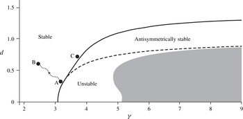
The set of steady-state doubly symmetric (in shape) hetons constructed by Makarov et al. (Reference Makarov, Sokolovskiy and Kizner2012) subdivides into three classes, namely, the generally stable, antisymmetrically stable and unstable hetons (figure 1). Here we track the evolution of two hetons labelled A and C in figure 1. Heton A is weakly stable in both senses, and heton B is substantially stable to antisymmetric perturbations but weakly stable in the general sense.
First we test heton A, whose coordinates on the (
 $\unicode[STIX]{x1D6FE}$
,
 $d$
)-plane are
 $\unicode[STIX]{x1D6FE}=3.2$
and
 $d=0.3$
. Due to its closeness to the stability bounds with respect to both asymmetric and antisymmetric perturbations (figure 1), this equilibrium might be disrupted by a small-amplitude perturbation, whether asymmetric or antisymmetric. Aiming to explain the observations made in the
 $\unicode[STIX]{x1D6FD}$
-plane simulations of modon transitions, we focus on antisymmetric perturbations using the version of the contour dynamics, which does not violate the antisymmetry of the upper- and lower-layer PV patches about the translation axis (see the reasoning in § 1).
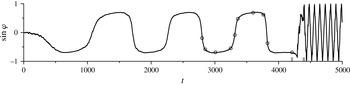
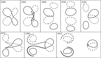
The accumulated effect of the antisymmetric numerical noise manifests itself in developing an oscillation (figure 2) with almost periodical stretching and cross-over of the upper and lower PV patches and subsequent regaining of their initial shape and mutual arrangement. This behaviour culminates in a transition, which occurs after a few complete oscillation cycles. More specifically, in the end of the last oscillation cycle, at the highest stage of the cross-over overlap of the front parts of the two vortices, the stretching becomes especially strong. Consequently, the bigger part of the upper-layer vortex captures the frontal part of the lower-layer PV patch (and vice versa), tears and advects it round (figure 3). This advection ends up with discharging of the detached vortices backwards. As a result, two vortex pairs emerge, a pair of weakly interacting vortices (on the left) and a new moving heton (on the right) with a less overlap than in the initial heton. Originally, the overlap of the almost circular upper- and lower-layer PV patches in heton A is pretty strong (figure 4 a). Therefore, it is no wonder that the evolution of heton A shares some traits with that of an unstable static (i.e. fully overlapping) circular columnar two-layer vortex induced by a finite-amplitude mode-2 perturbation, as described by Helfrich & Send (Reference Helfrich and Send1988).
Existence, stability and transitions of hetons. Shaded is the region in the (
 $\unicode[STIX]{x1D6FE}$
,
 $d$
)-plane, where no antisymmetric hetons are found. The solid and dashed lines are the bounds of stability to general (asymmetric) and antisymmetric perturbations, respectively. The region above the upper stability bound is populated by unconditionally stable hetons; the region between the two stability bounds is occupied by hetons that are stable to antisymmetric perturbations but unstable to asymmetric perturbations, and the region below the lower stability bound, by hetons unstable to the both types of perturbations. The two solid circles represent the original heton with
 $\unicode[STIX]{x1D6FE}=3.2$
and
 $d=0.3$
(labelled A) exposed to antisymmetric external noise, and the heton with
 $\unicode[STIX]{x1D6FE}\approx 2.45$
and
 $d\approx 0.6$
(labelled B), around which oscillates the heton resulting from the transition made by heton A. The dotted arrowed sinuous line symbolizes the transition from A to B. The solid circle with
 $\unicode[STIX]{x1D6FE}\approx 3.7$
and
 $d=0.7$
(labelled C) represents the heton, which makes a transition into a carousel tripole induced by asymmetric noise. This figure is an adaptation of figure 4(b) from Makarov et al. (Reference Makarov, Sokolovskiy and Kizner2012) with some additions and
 $\unicode[STIX]{x1D6FE}$
scaled according to the definition of
 $L$
given in § 2.

Heton-to-heton transition (A to B in figure 1) in a simulation with antisymmetric perturbations. Sine of the angle
 $\unicode[STIX]{x1D711}$
between the axis of translation and the longest chord of the biggest upper-layer PV patch. The transition event (see figure 3) occurs within the time interval from
 $t=4280$
to
 $t=4412$
indicated by two grey upward tick marks. Open circles indicate the states passed by heton A in the final cycle of the pre-transition oscillation (the corresponding shapes are shown in 4
a), and the state just before the beginning of the transition.

Heton-to-heton transition. Succession of shapes taken by the PV patches and filaments during the time interval from
 $t=4280$
to
 $t=4412$
(indicated in figure 2 by two grey upward tick marks), in which the transition from heton A to heton B occurs. Solid and dashed lines are the contours bounding the upper- and lower-layer PV patches, respectively; time is indicated in the upper-left corner of each plot.

After the splitting of the PV patches, in figure 2, we track the heton arranged by the bigger vortices, which moves very orderly in the same direction as heton A. The new heton is not an exact equilibrium, but is close to a steady-state heton labelled B in figure 1 and determined by
 $d\approx 0.6$
and
 $\unicode[STIX]{x1D6FE}\approx 2.45$
. These estimates of
 $d$
and
 $\unicode[STIX]{x1D6FE}$
are found as the mean separation between the PV patches and the patch size in the new heton, and its size, which is approximately 76 % of the original size of heton A. Heton B has a higher separation and a lesser overlap than A, i.e. is more distant from the stability bound on the parameter plane (figure 1), thus possessing higher stability. As any non-dissipative dynamical system, which is not in a steady state but is close to a stable equilibrium, the new heton oscillates in the vicinity of heton B. This correlates with the situation on the
 $\unicode[STIX]{x1D6FD}$
-plane, where the modon that forms as a result of a transition from a highly overlapping modon moves quasi-steadily, while performing some slowly damping oscillations (Kizner et al.
Reference Kizner, Berson and Khvoles2002; Khvoles et al.
Reference Khvoles, McWilliams and Kizner2007).
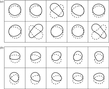
Examination of the shapes taken by the PV patches before and after the transition reveals a fundamental difference between the two oscillations. As noted above, before the transition, the perturbation consists in a nearly periodical stretching and tilting of the upper and lower PV patches within approximately
 $\pm 50^{\circ }$
(figures 2 and 4
a). During one period of this oscillation, approximately within 1000 time units (figure 2), the heton travels the distance of about 40
 $L$
. One cycle of the post-translation oscillation near heton B appears as turning by
 $360^{\circ }$
of a protuberance on the PV contour in each layer (figure 4
b). The period of this running-round oscillation, approximately 85 time units, is much shorter than the period of the pre-transition oscillation (figure 2), and is four times as long as the time it takes for a fluid parcel located at the patch boundary to make a complete revolution. Thus, most significant in this oscillation is not the mass transfer, but just the fluctuations in the PV distribution; in other words, the post-transition oscillation proceeds in a wave-like manner.
When comparing the frequencies of the two oscillations, a qualitative analogy with a mechanical pendulum suggests itself. We surmise that the low frequency of the pre-transition oscillation (relative to that of the post-transition one) is mostly due to the bigger size of heton A and to the elongation of its PV patches in the course of oscillation.
Succession of shapes (from top left to bottom right) (a) within the final cycle of the pre-transition, elongation–tilt oscillation (the corresponding phases are indicated in figure 2 by open circles), and (b) within one cycle of the post-transition, running-round oscillation. Lines as in figure 3.

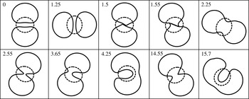
We now turn to the heton-to-tripole transition. Collision of two equal finite-core hetons sometimes results in the formation of a tripole (Sokolovskiy & Carton Reference Sokolovskiy and Carton2010). However, a tripole can also emerge due to the breakdown of a single barotropic dipole (Makarov & Kizner Reference Makarov and Kizner2011) or a heton, as shown below (figures 5 and 6). To initiate a simulation we take a heton with
 $\unicode[STIX]{x1D6FE}\approx 3.7$
and
 $d=0.7$
(labelled C in figure 1). This heton is stable to asymmetric perturbations, but is located close to the general-stability bound. Long-lasting exposure of the heton to small asymmetric perturbations of the PV contours gives rise to the formation of a baroclinic tripole.
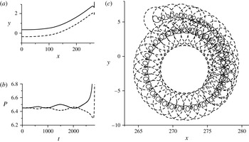
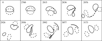
Initially, the accumulation of the effect of perturbations leads to bending of the heton trajectory (figure 5 a) and to the development of a low-frequency oscillation of the tilt type, visible in the graphs of the perimeters of the two patches versus time (figure 5 b). The growth of this oscillation culminates in splitting of the heton into two asymmetric hetons; subsequently, the two hetons collide making up the tripole (figure 6). Due to considerable filamentation during the transition and loss of PV, the resulting tripole acquires non-zero total circulation. So, the tripole’s motion can be described as a superposition of an orbital motion of the tripole as a whole, its own rotation and some oscillation in the mutual arrangement of three vortices (figure 5 c).
Transition of a doubly symmetric heton (labelled C in figure 1) into a carousel tripole in a simulation with asymmetric numerical noise. (a) Trajectories of the centroids of the upper- and lower-layer vortices before the transition. (b) Perimeters of the PV patches versus time before and at the beginning of the transition. (c) Trajectories of the centroids of the upper-layer core and one of the lower-layer satellites of the tripole that results from the transition. The (
 $x$
,
 $y$
)-coordinate system is related to the axis of antisymmetry and the transverse axis of the original heton. Lines as in figure 3.

Transition of a doubly symmetric heton into a carousel tripole. The original unperturbed heton (top left) and the succession of shapes taken by the PV patches and most pronounced filaments during the formation of a tripole. Lines and time as in figure 3.

In the both simulations presented above, before and after the transitions, the surgery is hardly involved; for this reason, the error in preservation of the integral invariants of motion does not exceed 0.01 %. However, the impetuous events that take place during the transitions necessarily affect the invariants, since at this time, strong PV filamentation occurs, thin filaments and debris are removed, and some far-scattered PV patches are just excluded from the consideration.
4 Tripole transitions
Depending on the shape of the satellite vortices (we place them in the lower layer), the steady-state uniform-PV doubly symmetric carousel tripoles can be categorized as either leaf-like or bean-like tripoles (Shteinbuch-Fridman et al.
Reference Shteinbuch-Fridman, Makarov, Carton and Kizner2015). At
 $\unicode[STIX]{x1D6FE}<2.905$
, only leaf-like steady states exist. In the
 $\unicode[STIX]{x1D6FE}\rightarrow 0$
limit, the flows in the two layers become independent of one another, being governed by barotropic equations each. Therefore, in this limit, the lower-layer vortices behave as a pair of identical vorticity patches whose motion was first investigated by Saffman & Szeto (Reference Saffman and Szeto1980); see also Saffman (Reference Saffman1992) and references therein. At
 $\unicode[STIX]{x1D6FE}>3.488$
and at moderate values of
 $d$
, only bean-like tripoles exist. In another limit,
 $\unicode[STIX]{x1D6FE}\rightarrow \infty$
, the streamlines in the layers become identical, so the shapes of the core and satellite vortices in a carousel tripole solution should look as if the tripole is barotropic; for instance, the core and satellites of such a tripole cannot overlap. This explains why the solutions obtained at large
 $\unicode[STIX]{x1D6FE}$
by Shteinbuch-Fridman et al. (Reference Shteinbuch-Fridman, Makarov, Carton and Kizner2015) are similar in shape to the barotropic tripoles observed in laboratory experiments (e.g. van Heijst & Kloosterziel Reference van Heijst and Kloosterziel1989; van Heijst et al.
Reference van Heijst, Kloosterziel and Williams1991) and to the semi-analytical solutions by Kizner & Khvoles (Reference Kizner and Khvoles2004a
,Reference Kizner and Khvoles
b
) and Kizner et al. (Reference Kizner, Khvoles and McWilliams2007). For a more detailed discussion of the two limits,
 $\unicode[STIX]{x1D6FE}\rightarrow 0$
and
 $\unicode[STIX]{x1D6FE}\rightarrow \infty$
, see Makarov et al. (Reference Makarov, Sokolovskiy and Kizner2012) and Shteinbuch-Fridman et al. (Reference Shteinbuch-Fridman, Makarov, Carton and Kizner2015). In the interval
 $2.905<\unicode[STIX]{x1D6FE}<3.488$
, both leaf-like and bean-like solutions are found. Below, we show that the transitions that slightly perturbed weakly stable tripoles can make depend greatly on which of these three intervals is considered.
Shteinbuch-Fridman et al. (Reference Shteinbuch-Fridman, Makarov, Carton and Kizner2015) studied numerically the stability of finite-core carousel tripoles to general-type (asymmetric) perturbations. Now, to better understand what routs the evolution of a weakly stable tripole might take, we check, in addition, the ‘symmetric stability’ i.e. the stability to perturbations that do not break the central symmetry of the tripoles. Clearly, any tripole, which is stable to general perturbations is stable to symmetric perturbations, but the opposite is not true. Therefore, as with hetons, the bounds of stability to the perturbations of the first and second type should not necessarily coincide. For tripoles, the greatest difference in the stability bounds is observed in the interval
 $2.905<\unicode[STIX]{x1D6FE}<3.488$
, where the leaf-like and bean-like tripoles coexist, and baroclinicity is most significant. For
 $\unicode[STIX]{x1D6FE}<2.905$
, the two stability bounds approach each other as
 $\unicode[STIX]{x1D6FE}$
decreases, and similarly for
 $\unicode[STIX]{x1D6FE}>3.488$
as
 $\unicode[STIX]{x1D6FE}$
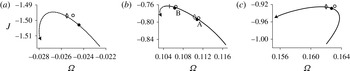
increases. This can be seen in figure 7 in which, as an example, the families of steady-state tripole solutions at
 $\unicode[STIX]{x1D6FE}=1$
, 3.4 and 5 are shown by curved lines on the (
 $\unicode[STIX]{x1D6FA}$
,
 $J$
)-plane made by the tripole’s angular velocity
 $\unicode[STIX]{x1D6FA}$
and angular momentum
 $J$
. Diamonds and short vertical bars on these lines mark the bounds of stability to general-type and symmetric perturbations, respectively; bold and empty circles indicate, respectively, the steady and perturbed tripoles used to initialize our simulations; arrows mark the marginal solutions, in which the satellite vortices touch each other. Note that, in the
 $\unicode[STIX]{x1D6FE}=1$
and 5 cases, the two stability bounds are indistinguishable.
The tripoles chosen for simulations possess some ‘margin of safety’, so that the asymmetric noise coming from the numerical code is insufficient to induce a true transition. Instead, it leads to smooth and slow growth in the separation between the core and the satellites, i.e. to slow ‘creeping’ of a tripole in the manifold of steady-state solutions towards a more stable equilibrium. Therefore, in order to initiate a transition, we impose an initial perturbation on an original equilibrium state.
Families of steady-state carousel tripoles on the (
 $\unicode[STIX]{x1D6FA}$
,
 $J$
)-plane at (a)
 $\unicode[STIX]{x1D6FE}=1$
, (b)
 $\unicode[STIX]{x1D6FE}=3.4$
, and (c)
 $\unicode[STIX]{x1D6FE}=5$
. Leaf-like and bean-like tripoles are shown by dashed and solid lines, respectively. Arrows mark marginal tripoles in which the two satellite vortices touch each other; short bars and diamonds mark the bounds of stability to symmetric and asymmetric perturbations, respectively (indistinguishable in a,c); unstable states are located to the left of the stability bounds; the states located in (b) between the bar and the diamond are stable to symmetric but unstable to asymmetric perturbations. Solid circles indicate the steady states subjected to initial perturbations, and open circles, the perturbed tripoles used to initialize the numerical simulations. In (b), the tripoles chosen for simulations are labelled A (generally stable) and B (symmetrically stable).

The initial perturbation consists in shortening, by a small value
 $\unicode[STIX]{x1D700}$
, the separation between the centroids of the core vortex and of each of the satellite vortices without changing the shapes of the PV patches. In the perturbed tripoles, the linear momentum and total PV remain unchanged, but the parameters
 $d$
,
 $\unicode[STIX]{x1D6FA}$
and
 $J$
do change to some extent. When
 $\unicode[STIX]{x1D700}$
is sufficiently small, the perturbed tripole undergoes oscillations without a structural change; this testifies to the tripole’s stability. By increasing
 $\unicode[STIX]{x1D700}$
we seek out the critical perturbation strength,
 $\unicode[STIX]{x1D700}_{CR}$
, above which the perturbation ultimately leads to the satellites’ merger and to a transition to a new non-tripole configuration.
When presenting the results related to tripoles, it is useful to renormalize time, taking the period of revolution of the unperturbed stationary tripole as the time unit. In contrast to what we did in § 3, below, the upper-layer contours are shown by a dashed line, and the lower-layer contours, by a solid line. This is because, in the simulations initialized by tripoles, the shape of the upper-layer (core) vortex barely changes, and the most important events occur in the lower layer. Oscillations and transitions are tracked through monitoring the total perimeter
 $P$
of the lower-layer PV patches. Although the initial perturbations of the tripoles are always symmetric, in all the simulations discussed below, we use the standard version of the contour-surgery algorithm which is not supposed to preserve any symmetry. The errors in conservation of the quantities that, in theory, should be integral invariants, remain within fractions of a per cent for hundreds of normalized time units (since the linear momentum of a steady-state tripole is zero, we track it separately for the core and each of the satellites).
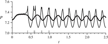
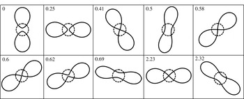
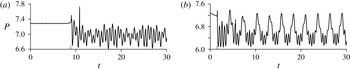
Evolution of a weakly stable tripole at
 $\unicode[STIX]{x1D6FE}=1$
(see figure 7
a) initiated by shortening the separation by
 $\unicode[STIX]{x1D700}$
. The total perimeter of the lower-layer PV patches versus time. Bold line,
 $\unicode[STIX]{x1D700}=0.0019202$
; thin line,
 $\unicode[STIX]{x1D700}=0.001920201$
. The times of the first merger of the lower-layer PV patches and of the three separation–merger events are indicated by grey upward marks.

Formation of an almost doubly symmetric hourglass shape from a perturbed (
 $\unicode[STIX]{x1D700}=0.001920201$
) tripole with
 $\unicode[STIX]{x1D6FE}=1$
and
 $d=0.815$
(see figure 7
a). Succession of shapes in a simulation that was run using the conventional code (i.e. without imposed preservation of any symmetry). The dashed and solid lines are the contours bounding the upper- and lower-layer PV patches, respectively; time is indicated in the upper-left corner of each frame. The corresponding evolution of
 $P$
is shown in figure 8.

We begin with the case where
 $\unicode[STIX]{x1D6FE}=1$
(figure 7
a). In the tripole used for the simulation, the unperturbed separation is
 $d=$
0.815, and the rotation is satellite dominated, i.e. clockwise. At the critical perturbation strength,
 $\unicode[STIX]{x1D700}_{CR}=0.0019202$
, the tripole oscillates around the original stationary tripole state (bold line in figure 8), but an increase of
 $\unicode[STIX]{x1D700}$
by just
 $10^{-9}$
changes the tripole behaviour significantly (thin line in figure 8). For a quarter of a revolution period, from
 $t=0$
to
 $t=0.25$
, the bold and thin lines in figure 8 go close to each other. Then the satellites’ perimeter increases rapidly (the thin line deviates from the bold one). The latter means that the satellites become more and more stretched; from this point, the transition begins. The initial state and the succession of shapes taken by the PV patches by
 $t=2.32$
are provided in figure 9. In fact, the simulation lasted for a much longer time than is shown in figures 8 and 9, and the integral invariants were preserved to a high accuracy; also the angular velocity of the vortex structure barely changed.
At
 $t=0.41$
the satellites merge forming a single hourglass-shaped patch (figure 9). Thereafter by
 $t=1$
, for three times, the lower-layer PV structure again takes on the form of two leafs with non-touching sharp tips (figures 8 and 9). After the lapse of one revolution period, the process stabilizes in a quasi-periodic oscillation of the rotating hourglass structure. In figure 8, the crest in the perimeter oscillation corresponds to the minimum ‘waist’ thickness, which is close to zero (e.g. frame
 $t=2.23$
in figure 9), while the trough, to the maximum waist thickness (e.g. frame
 $t=2.32$
in figure 9). The shape of the upper-layer core vortex also oscillates, but with a substantially lesser amplitude. The configuration resulting from the transition is almost doubly symmetric.
The repeated merger and splitting of the lower-layer vortices observed in this simulation resembles the behaviour of two identical barotropic vortices (Saffman & Szeto Reference Saffman and Szeto1980; Dritschel Reference Dritschel1986, Reference Dritschel1995; Saffman Reference Saffman1992). This is natural, taking into account the fact that the smaller
 $\unicode[STIX]{x1D6FE}$
, the weaker the interaction between the flows in the two layers. In the barotropic case, reduction below some critical value of the separation between two like symmetrically arranged vortices leads to their merger and to the formation of a quasi-elliptical vortex. The reverse process of splitting of a slightly perturbed sufficiently elongated elliptic vortex into a couple of nearly identical vortices was first described by Dritschel (Reference Dritschel1986).
Next we consider the case of
 $\unicode[STIX]{x1D6FE}=3.4$
, where both the leaf-like and bean-like steady-state tripoles exist and rotate counterclockwise, and the bounds of stability to general (asymmetric) and centrally symmetric perturbations differ noticeably from one another (figure 7
b). The tripoles located on the parameter plane between the two bounds are stable to symmetric perturbations, but unstable in the general sense. Therefore, if a simulation is run with the code that preserves the central symmetry, small initial perturbations imposed on the intermediate tripoles will not grow. However, when the conventional code is used to simulate the evolution of such a tripole (this is what is done in fact), asymmetric numerical noise will necessarily lead to unstable developments and to growing asymmetry of the vortex structure. More or less similar evolution can be expected if a tripole, which is weakly stable in the general sense, is moved away from the equilibrium by a small initial perturbation: the accumulation of the effect of asymmetric numerical noise will take the tripole into the intermediate range, thus causing unstable behaviour of the tripole. Below, the evolution of two initially perturbed tripoles is discussed (figures 10–12). The first of these tripoles is weakly stable to general-type perturbations, and the second one is weakly stable to symmetric perturbations (labelled, respectively, A and B in figure 7
b).
Evolution of two weakly stable tripoles at
 $\unicode[STIX]{x1D6FE}=3.4$
(see figure 7
b), initiated by shortening the separation by
 $\unicode[STIX]{x1D700}$
. The total perimeter of the lower-layer PV patches versus time in simulations that were run using the conventional code. (a) The tripole with
 $d=0.554$
(labelled A in figure 7
b), stable to general-type perturbations;
 $\unicode[STIX]{x1D700}=0.001108$
. (b) The tripole with
 $d=0.545$
(labelled B in figure 7
b), stable to centrally symmetric perturbations;
 $\unicode[STIX]{x1D700}=0.00122625$
. The moments of the transitions to non-tripole configurations are indicated by grey upward tick marks.


Transition of the tripole labelled B in figure 7(b) (
 $\unicode[STIX]{x1D700}=0.00122625$
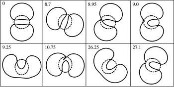
) to an oscillating horseshoe–hourglass regime. Succession of shapes in a simulation that was run using the conventional code. The corresponding evolution of
 $P$
is shown in figure 10(b). Lines and time as in figure 9.

In figures 10(a) and 11, a transition of a tripole to a horseshoe configuration is shown. The initial state for this simulation is obtained through shortening the separation in tripole A (with
 $\unicode[STIX]{x1D6FE}=3.4$
and
 $d=0.554$
) by
 $\unicode[STIX]{x1D700}=0.001108$
; an increase of
 $\unicode[STIX]{x1D700}$
above this value accelerates the onset of the transition, but does not change the sequence of events. At the first stage of evolution, a low-amplitude oscillation in the vicinity of the original steady state A occurs, which is evidenced by some quite regular fluctuations of the total perimeter of the lower-layer PV (figure 10
a). However, at this stage, the tilt of the satellites with respect to one another gradually increases (frame
 $t=8.7$
in figure 11). This leads to the merger of the two asymmetric satellites by approximately
 $t=8.95$
–9.0 (grey upward tick mark on the
 $t$
-axis in figure 10
a) and to the emergence of an oscillating horseshoe-shaped structure, which rotates with almost the same angular velocity as the original unperturbed tripole. In figures 10(a) and 11, only the first few tens of rotation cycles are shown. In fact, the computations were terminated at
 $t=510$
, and no visible changes in the behaviour of the horseshoe-shaped structure were detected within approximately 500 cycles of its rotation. The overall rotation and oscillation of the vortex structure is accompanied by slow translational motion. The latter is due to the contour surgery, which is most active during the time interval
 $8.5<t<11.5$
. We note, however, that the changes in the invariants of motion, including the total areas of the upper- and lower-layer PV patches, do not exceed 0.1 %. A transition to an asymmetric structure due to the merger of the satellites was first observed by Polvani & Carton (Reference Polvani and Carton1990) in some of their barotropic tripoles obtained with a contour-surgery algorithm and perturbed by a random displacement of each of the nodes on the equilibrium vorticity contours.
Evolution of a weakly stable tripole at
 $\unicode[STIX]{x1D6FE}=5$
(see figure 7
c), initiated by shortening the separation by
 $\unicode[STIX]{x1D700}$
. The total perimeter of the lower-layer PV patches versus time. Bold line,
 $\unicode[STIX]{x1D700}=0.0010868$
; thin line,
 $\unicode[STIX]{x1D700}=0.0010869$
. The moments of closure and opening of the lower-layer ring are indicated by grey upward tick marks.

The transition made by tripole B (
 $\unicode[STIX]{x1D6FE}=3.4$
,
 $d=0.545$
and
 $\unicode[STIX]{x1D700}=0.00122625$
) is shown in figures 10(b) and 12. In this simulation, the transition is to a quasi-periodic regime, in which the horseshoe and hourglass shapes (corresponding, respectively, to the crests and troughs in figure 10
b) are taken successively. This periodic change in shape is observed till the termination of the computations at
 $t=500$
. By this time the vortex structure makes some 300 complete rotations while oscillating. Since the original, unperturbed tripole is unstable to asymmetric perturbations, independently of
 $\unicode[STIX]{x1D700}$
, no oscillation around a steady-state tripole occurs before the transition; the magnitude of the initial perturbation affects only how quickly the satellites merge.
The last case in this series is
 $\unicode[STIX]{x1D6FE}=5$
, in which only bean-like steady-state tripoles exist and rotate counterclockwise. The separation in the original weekly stable steady-state tripole taken for simulation is
 $d=0.575$
, and the critical perturbation strength is
 $\unicode[STIX]{x1D700}_{CR}=0.0010868$
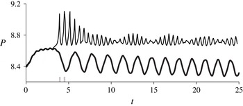
. At
 $\unicode[STIX]{x1D700}=\unicode[STIX]{x1D700}_{CR}$
, the tripole oscillates close to the original steady state with a slowly decaying amplitude (figure 13, bold line), but an increase of
 $\unicode[STIX]{x1D700}$
by
 $10^{-7}$
changes the behaviour. This becomes evident after
 $t=3$
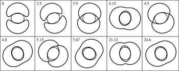
, when the thin and bold lines in figure 13 diverge. The two-sided merger of the satellites (figure 14) occurs at about
 $t=3.9$
(the left grey tick mark in figure 13) when their tips come in contact, and shortly after that a well-pronounced ring vortex (though non-circular) is formed in the lower layer (frame
 $t=4.15$
in figure 14). So, one may speak now about the formation of a two-layer ringed (or shielded) monopole. The ring opens for a while (frame
 $t=4.5$
in figure 14; the right grey upward tick mark in figure 13). Then, by
 $t=7$
, a slowly decaying modulated quasi-periodic regime is reached, in which the ringed monopole oscillates between the shapes shown in the frames
 $t=21.12$
and
 $t=24.6$
in figure 14. The error in preserving the integral invariants in this simulation is under 0.5 %.
The bounds of stability to the both types of perturbations nearly coincide at
 $\unicode[STIX]{x1D6FE}=5$
(figure 7
c). In this respect, the case
 $\unicode[STIX]{x1D6FE}=5$
is akin to
 $\unicode[STIX]{x1D6FE}=1$
. For example, despite the fact that the numerical noise is asymmetric, the vortex structures in the first and the last simulations remain virtually doubly symmetric.
In barotropic flows, the formation of a tripole or higher multipoles from a shielded monopole was discussed in a number of publications based on laboratory experiments and numerical simulations (for references see § 1). Likewise, it has been known that unstable evolution of a two-layer isolated columnar or shielded monopole can result in the formation of more complex structures, including tripoles (e.g. Kozlov et al. Reference Kozlov, Makarov and Sokolovskiy1986; Flierl Reference Flierl1988; Helfrich & Send Reference Helfrich and Send1988; Carton & Correard Reference Carton, Correard and Sorensen1999; Baey & Carton Reference Baey and Carton2002). A reverse tendency of a barotropic tripole towards the formation of a convoluted shape resembling a shielded monopole, as far as we know, was reported only once, by Polvani & Carton (Reference Polvani and Carton1990), who dealt with a strongly perturbed barotropic tripole with big satellites. In this present work, for the first time, the possibility is demonstrated for a transition from a weakly stable two-layer carousel tripole to a fundamentally robust ringed (shielded) monopole.
Formation of an almost doubly symmetric ringed (shielded) monopole from a perturbed (
 $\unicode[STIX]{x1D700}=0.0010869$
) tripole at
 $\unicode[STIX]{x1D6FE}=5$
and
 $d=0.575$
(see figure 7
c). Succession of shapes in a simulation that was run using the conventional code. The corresponding evolution of
 $P$
is shown in figure 13. Lines and time as in figure 9.

5 Conclusion
We considered quasigeostrophic two-layer finite-core uniform-PV hetons and carousel tripoles on the
 $f$
-plane. Simulations of the evolution of weekly stable hetons and tripoles exposed for a long time to small perturbations were performed with the use of the contour-surgery method. The focus was on the transitions and pre- and post-transition oscillations.
In hetons, two types of transitions were observed. In response to antisymmetric perturbations, a substantially overlapping (therefore, located close to the mutual bound of stability to antisymmetric and, generally, asymmetric perturbations) heton makes a transition to a new heton state. The transition is a culmination of a periodical stretching and tilting of the upper- and lower-layer PV patches of the heton. At a certain stage of the oscillation, when the stretching becomes especially strong, due to the cross-over overlap of the two patches, the frontal part of the vortex located in one layer is captured by the bigger part of the vortex residing in the other layer, teared away and advected backward. The pair of smaller, weakly interacting vortices formed by this means is then discharged, and what remains is a new unsteady heton which oscillates quasi-periodically around some steady-state heton equilibrium. This steady-state heton is smaller than the original one, but has a larger separation and a lesser overlap, thus being fairly stable. The results obtained with antisymmetrically perturbed hetons explain the mechanism of the transitions observed earlier in baroclinic modons on the
 $\unicode[STIX]{x1D6FD}$
-plane (overviewed in § 1). Asymmetric perturbations are shown to be able to induce a transition of a heton to a periodically oscillating tripole state.
Transitions in finite-core baroclinic tripoles, to the best of our knowledge, were not discussed so far. Our simulations show that a slightly perturbed weakly stable carousel tripole is able to make a transition to a new, non-tripole state due to the merger of the lower-layer satellites. The shape of the resulting vortex structure depends on the shape of the satellites in the original tripole (leaf-like or bean-like), which, in turn, is determined mostly by the size parameter
 $\unicode[STIX]{x1D6FE}$
. At low and high values of
 $\unicode[STIX]{x1D6FE}$
, the bounds of stability to symmetric and asymmetric perturbations go close to each other and only one scenario of transition is revealed, a transition to an hourglass structure at low
 $\unicode[STIX]{x1D6FE}$
, or to a ringed monopole at high
 $\unicode[STIX]{x1D6FE}$
. Noticeably, in these two cases, small asymmetric perturbations barely affect the overall double symmetry. In the intermediate range of
 $\unicode[STIX]{x1D6FE}$
, two variants of transition are observed. The route taken in the tripole evolution depends on whether the initial tripole is stable to general (asymmetric) perturbations, or to symmetric perturbations only. A tripole, which is weakly stable in the general sense, transits to an asymmetric horseshoe-shape structure. A tripole, which is stable to symmetric perturbations only, transforms into a fundamentally quasi-periodic regime, in which an oscillation between the hourglass and horseshoe shapes occurs.
The heton transitions discussed in § 3 are specifically baroclinic phenomena. In tripoles (§ 4), the effect of baroclinicity is highest in the intermediate range of
 $\unicode[STIX]{x1D6FE}$
. At smaller
 $\unicode[STIX]{x1D6FE}$
, the upper-layer vortex remains nearly circular, its interaction with the lower-layer satellites being weak. Thus the behaviour of the lower-layer vortices recalls that of a couple of like barotropic vortices. In the simulation, in which the transition to a ringed monopole is observed, the upper- and lower-layer PV patches hardly overlap, that is, behave in a barotropic-like manner. A tripole-to-monopole transition in two-layer flows has not been reported up to date. Regarding barotropic tripoles, we are aware of only one publication where a scenario of this kind was discussed (Polvani & Carton Reference Polvani and Carton1990). Such a transition, however, is consistent with the tendency of multipolar vortices to transform into less complex configurations. This has been observed in numerical simulations (Morel & Carton Reference Morel and Carton1994) and laboratory experiments (Trieling et al.
Reference Trieling, van Heijst and Kizner2010). As one of the lines of our future work, we plan an extensive study of the mutual transitions of monopoles and tripoles in terms of dynamical systems, by examining the fixed points in a parameter space and of the trajectories in which unsteady vortex structures move.
Acknowledgements
Z.K. and B.S.-F. acknowledge the financial support of this research by the Binational Israel–US Science Foundation (BSF), grant 2014206.