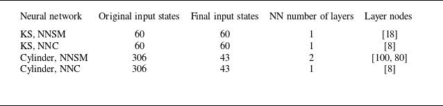
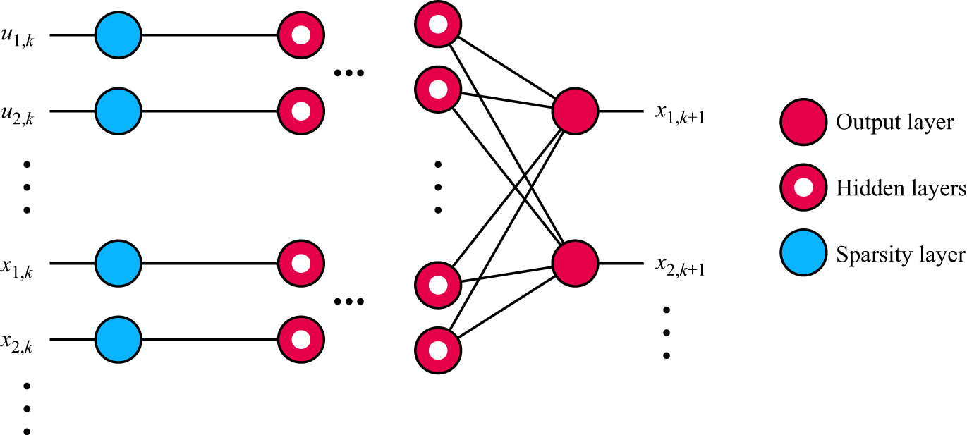
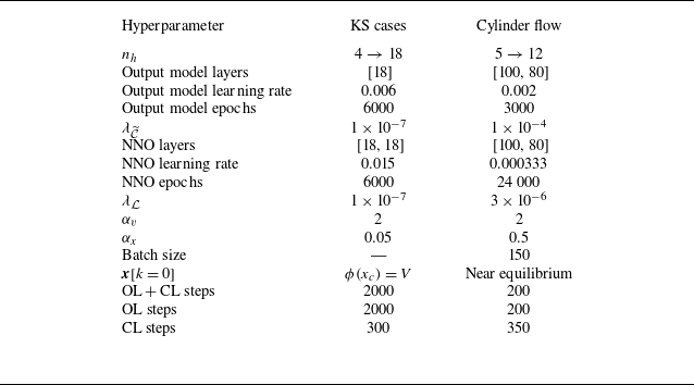
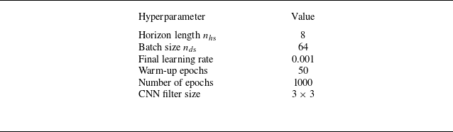
1. Introduction
Active control of fluidic systems is a challenging task, partly due to complex nonlinear phenomena and high dimensionality. Closed-loop flow control requires particular attention to challenges related to sensor placement, data acquisition systems, real-time adjustable actuators and sampling specifications (e.g. sensor bandwidth, noise levels and sampling frequency), which are often limited by cost and technological limitations. Frameworks commonly studied in flow sciences, such as resolvent analysis, machine learning and network analysis often serve as effective tools for designing control algorithms (Gad-el Hak Reference Gad-el Ha2001; Brunton & Noack Reference Brunton and Noack2015; Brunton, Noack & Koumoutsakos Reference Brunton, Noack and Koumoutsakos2020; Taira & Nair Reference Taira and Nair2022; Audiffred et al. Reference Audiffred, Cavalieri, Brito and Martini2023).
Resolvent analysis has been combined with experimental set-ups to model fluidic systems and design optimal controllers. For instance, Audiffred et al. (Reference Audiffred, Cavalieri, Brito and Martini2023) achieved the attenuation of flow unsteadiness using plasma actuators to cancel incoming Tollmien–Schlichting waves. Although their set-up did not involve feedback control, a feedforward resolvent-based methodology was proposed to find an optimal causal control kernel via the Wiener–Hopf formalism. The experimental results showed that the approach is capable of promoting better attenuations compared with direct cancellation through transfer function inversion, which requires truncation to a causal kernel that leads to suboptimal solutions.
The development of learning techniques is also leveraged in the field of experimental flow control. Fan et al. (Reference Fan, Yang, Wang, Triantafyllou and Karniadakis2020) developed a closed-loop control system using reinforcement learning to maximise power gain efficiency in a cylinder flow by evaluating the states that comprise the drag and lift coefficients. Their actuation set-up used smaller rotating cylinders in the wake, enabling considerable drag reduction.
In recent studies, researchers explored new control concepts through numerical simulations, which provide controlled environments with access to variables that are often inaccessible in experiments. Rabault et al. (Reference Rabault, Kuchta, Jensen, Réglade and Cerardi2019), Ren, Rabault & Tang (Reference Ren, Rabault and Tang2021), Castellanos et al. (Reference Castellanos, Cornejo Maceda, De La Fuente, Noack, Ianiro and Discetti2022), Varela et al. (Reference Varela, Suárez, vila, Francisco, Arnau, Jean, Bernat, Miguel, Lehmkuhl and Vinuesa2022) and Déda et al. (Reference Déda, Wolf and Dawson2024) employed machine learning techniques to control the flow past a confined cylinder and successfully achieved performance goals such as stabilisation and drag reduction. One of the set-ups used in these studies – which is also explored in the current work – makes use of minijets actuating in phase opposition, modulated by feedback of flow field velocity measurements. The machine learning algorithms proposed in these studies were shown to be powerful tools for controlling idealised flow systems. Closed-loop control, however, relied on feedback of wake velocity measurements, bypassing observability constraints that can arise in real-world set-ups, where technology limits the number and positioning of sensors. The impracticality of such a sensing approach motivates research on flow estimation under restricted sampling, where the system states must be inferred from a limited number of sensors with constrained placement and real-time measurement capabilities.
The control of turbulent flows within numerical environments has also been studied (Park & Choi Reference Park and Choi2020; Guastoni et al. Reference Guastoni, Rabault, Schlatter, Azizpour and Vinuesa2023). Sonoda et al. (Reference Sonoda, Liu, Itoh and Hasegawa2023) presented a neural network (NN) approach to perform continuous actuation along the walls of a turbulent channel flow. The proposed multi-layer perceptrons were fed with information locally related to the actuation point. In one of the studied cases, the flow was completely relaminarised, demonstrating the potential of machine learning techniques for flow control. Another way to leverage NNs for flow control was proposed by Morton et al. (Reference Morton, Witherden, Jameson and Kochenderfer2018), who modelled the dynamics of a cylinder flow through networks trained to learn state mappings to span a Koopman invariant subspace. Significant vortex shedding attenuation was achieved by feeding flow images into a convolutional neural network (CNN) model iterated through time within a finite horizon, which was used for model predictive control (MPC). Other techniques employed for flow control include network analysis for control design (Yeh, Meena & Taira Reference Yeh, Meena and Taira2021), sparse identification of nonlinear dynamics (SINDy) with control (Brunton, Proctor & Kutz Reference Brunton, Proctor and Kutz2016), online extremum seeking (Déda & Wolf 2022; Payne, Zhang & Cattafesta Reference Payne, Zhang and Cattafesta2024) and direct opposition control (Choi, Moin & Kim Reference Choi, Moin and Kim1994).
While these previous studies presented innovative control designs capable of accomplishing important goals, there are barriers that hinder their implementation in real-world systems. One of the most important limitations is the sensor set-up. In experiments, online sensing is usually limited to a few pressure and skin friction probes that need to be located along the walls, since velocity measurements in the flow field, e.g. through particle image velocimetry (PIV), can be both expensive and computationally prohibitive in real time. While velocity measurements with hotwire probes can be feasible for online sensing, these also only typically allow for a smaller number of sensors, and can be disruptive to the downstream flow field. For these reasons, open-loop control strategies are also often explored to manipulate fluid flows. In such cases, the optimisation of flow variables is done by tuning the actuator to work offline, regardless of the online flow signals. For example, through large-eddy simulations, Visbal & Benton (Reference Visbal and Benton2018), Ramos et al. (Reference Ramos, Wolf, Yeh and Taira2019) and de Souza et al. (Reference de Souza, Wolf, Safari and Yeh2025) studied the open-loop control of aerofoils under dynamic stall. By setting specific actuation frequencies for oscillatory jets near the leading edge, significant reductions were observed in the phase-averaged drag. Genetic algorithms (GAs) have also been applied in experimental studies to find the best actuation set-ups to optimise flow variables. Zigunov et al. (Reference Zigunov, Sellappan and Alvi2022a ) employed a GA to find a subset of actuators from a set of candidates to reduce drag in a flow over a bluff body, while Zigunov et al. (Reference Zigunov, Song, Sellappan and Alvi2023) used a similar approach to maximise the thrust vectoring angle in a supersonic jet. Raibaudo et al. (Reference Raibaudo, Zhong, Noack and Martinuzzi2020) used GAs to control the flow past a triangular array of cylinders known as a fluidic pinball, targeting either drag reduction or flow symmetry by setting the rotation speed of the cylinders. Another way to approach sensor limitations is by discovering optimal sensor placement to reduce the required number of probes. For example, Paris, Beneddine & Dandois (Reference Paris, Beneddine and Dandois2021) introduced a reinforcement learning approach to develop drag reduction control strategies while optimising sensor placement using an L0 regularisation scheme. Déda et al. (Reference Déda, Wolf and Dawson2024) trained NN models for control design using an L1 regularisation approach to reduce the number of sensors used to evolve the system states in time.
Flow reconstruction from limited sensor data is also an area of interest within fluid dynamics. Different techniques have been used to approach this problem, such as gappy proper orthogonal decomposition (Willcox Reference Willcox2006), a pivoted QR decomposition of an identified set of basis functions (Manohar et al. Reference Manohar, Brunton, Kutz and Brunton2018), data-driven dynamical models with Kalman filters (Sashittal & Bodony Reference Sashittal and Bodony2021; Graff, Medina & Lagor Reference Guastoni, Rabault, Schlatter, Azizpour and Vinuesa2023), and decoder NNs (Williams, Zahn & Kutz Reference Williams, Zahn and Kutz2022). Mousavi & Eldredge (Reference Mousavi and Eldredge2025) and Fukami et al. (Reference Fukami, Iwatani, Maejima, Asada and Kawai2025) developed encoder NNs to map complex flow fields to reduced latent spaces, enabling the low-dimensional sensor-based estimation of features. Their approach facilitated sensor sensitivity analyses, allowing for finding the most relevant directions in the sensor space. Nair & Goza (Reference Nair and Goza2020) utilised fully connected NNs to identify reduced states over time and then employed reduced-order models to map these states back to the high-dimensional state space. Turbulent channel flow reconstruction from wall probes that read pressure and shear stresses was performed by Nakamura & Fukagata (Reference Nakamura and Fukagata2022). Resolvent analysis is also a powerful tool for flow reconstruction. Its applications include the inference of statistical properties and reconstruction of flow fields, also allowing for causal approximations of the relevant transfer functions, either through truncation of optimal kernels or by optimal modelling through a Wiener–Hopf procedure (Martini et al. Reference Martini, Cavalieri, Jordan, Towne and Lesshafft2020; Towne, Lozano-Durán & Yang Reference Towne, Lozano-Durán and Yang2020; Amaral et al. Reference Amaral, Cavalieri, Martini, Jordan and Towne2021).
Reconstruction problems such as estimating velocity fields from particle images and super-resolution have also been investigated (Morimoto et al. Reference Morimoto, Fukami, Zhang and Fukagata2022; Miotto, Wolf & Zigunov Reference Miotto, Wolf and Zigunov2025). The latter approach involves techniques developed for upscaling low-resolution flow images (Fukami, Fukagata & Taira Reference Fukami, Fukagata and Taira2023). The super-resolution analysis of the flow past two cylinders distanced by a varying gap was done by Morimoto et al. (Reference Morimoto, Fukami, Zhang and Fukagata2022), where low-resolution images are upscaled using CNNs to provide a flow field with finer details. Fukami, Fukagata & Taira (Reference Fukami, Fukagata and Taira2019) implemented a NN architecture that combines a CNN upscaler with downsampled skip connections and a CNN with multiscale filters to infer details of a turbulent flow. Page (Reference Page2024) proposed a super-resolution estimation approach where NNs are trained using backpropagation through time (BPTT) without the need for high resolution reference data by leveraging a differentiable dynamic flow model. Starting from a coarse initial condition, their approach stores memory from past estimations and produces accurate flow estimations after a few iterations over time.
In the present work we approach flow estimation from limited sensor data by leveraging topologies commonly used in control theory. For example, two well-established state estimation approaches integral to modern control theory are the Luenberger observer and the Kalman filter. Taking inspiration from such approaches, we propose a dynamic estimation of the flow variables – as opposed to a static reconstruction – by leveraging models with memory signals that correspond to the plant state space. The implementation of closed-loop NN-based state observers, or simply neural network observers (NNOs), can be done through approaches analogous to neural network controllers (NNCs). Déda et al. (Reference Déda, Wolf and Dawson2024), for example, proposed the training of NNCs via BPTT, where the controller is trained to stabilise a neural network surrogate model (NNSM) by approaching an equilibrium point within a finite-time horizon. A similar framework was presented by Yadaiah & Sowmya (Reference Yadaiah and Sowmya2006), who leveraged BPTT to train state observers for simple plants. By testing their technique with low-dimensional nonlinear systems, the authors showed that the NNs were able to outperform implementations of the extended Kalman filter (EKF).
Here, we propose the implementation of NNOs to enable dynamic output feedback control of flows by dynamically estimating states from limited sensor data. To do so, we leverage previously trained NNSMs, which contain states whose sensing is not feasible in real-world systems. Instead of assuming online feedback of the states, we leverage data from more realistic sensors to infer the states required to feed the controllers. The present methodology is inspired by the Luenberger observer, but machine learning tools are used to replace the systems from the traditional linear approach, which can present prohibitive limitations when working with strongly nonlinear systems such as fluid flows. Other approaches for the generalisation of the Luenberger observer include the application of NNs for learning mappings to provide a nonlinear observer considering continuous-time input-affine systems (Ramos et al. Reference Ramos, Wolf, Yeh and Taira2020). Furthermore, Zeitz (Reference Zeitz1987) and Afri et al. (Reference Afri, Andrieu, Bako and Dufour2016) reported extensions of the Luenberger observer applied to low-dimensional single-input single-output systems. In the realm of fluid flows, NNs can be used to provide more general approaches that are not necessarily limited to very strict assumptions. This comes, at the same time, with the cost of not providing formal convergence proofs, but the complex dynamics of unstable flows make it necessary to explore black-box techniques. Current literature provides estimation techniques that employ flow solvers or surrogate models to complete information by embedding dynamics (Zhong et al. Reference Zhong, Fukami, An and Taira2023; Page Reference Page2024).
The proposed framework is tested with three different nonlinear systems, namely a modified Kuramoto–Sivashinsky (KS) equation, a confined cylinder flow previously studied by Rabault et al. (Reference Rabault, Kuchta, Jensen, Réglade and Cerardi2019) and experimental data obtained from a turbulent boundary layer. The first two cases are tested within numerical simulations, and the observers are employed to estimate the states that are in turn fed to a pre-trained stabilising controller. Online sensing for state estimation is obtained assuming adverse conditions, such as insufficient sampling time to match the discrete plant model, reduced number of sensors and different types of random noise. For the boundary layer case, we use the experimental data provided by Zigunov (Reference Zigunov2020) to train all required NNs. For this set-up, specialised NN architectures are proposed to process PIV data. Low-resolution images of the flow velocities are employed for the estimation of flow variables, in an approach that differs from current super-resolution techniques by leveraging NNSM predictions. Since the available turbulent boundary layer dataset is from a previous experiment to which our group does not have access, the tests are restricted to flow state estimation without control. The remaining sections of the present work are organised as follows: § 2 discusses the methodology employed for flow state estimation through limited sensor data, § 3 presents the plant set-ups studied, § 4 reports the results obtained for each case and § 5 discusses the main achievements and limitations of the proposed methodology. In the scope of the present work, the terms ‘observer’ and ‘estimator’ are used interchangeably.
2. Methodology
In this section the mathematical tools utilised in the implementation of the NNOs are presented. First, a review on the discrete Luenberger observers is provided in § 2.1 to introduce the main ideas that inspired the choices regarding the NN approach. A nonlinear scheme analogous to the Luenberger observers is then presented in § 2.2. Finally, a modified structure for the estimator loop is introduced in § 2.3, in order to make the implementation feasible in the context of the studied systems. The training set-up for the NNOs is then presented. For a general overview on state observers, we refer the reader to Luenberger (Reference Luenberger2007) and Friedland (Reference Friedland2012) for a review on observers.
2.1. Discrete Luenberger observer
Consider the discrete-time invariant linear dynamical system described by
 \begin{align} \boldsymbol{x}[k+1] &= \unicode{x1D63C} \boldsymbol{x}[k] + \unicode{x1D63D} \boldsymbol{u}[k] , \\[-10pt] \nonumber \end{align}
 \begin{align} \boldsymbol{y}[k] &= \unicode{x1D63E} \boldsymbol{x}[k] , \\[10pt] \nonumber \end{align}
where
 $\boldsymbol{x}[k]$
is the state vector at discrete time
 $k$
,
 $\boldsymbol{u}[k]$
is the control input vector and
 $\boldsymbol{y}[k]$
is the measurable output vector. Matrices
 $\unicode{x1D63C}$
,
 $\unicode{x1D63D}$
and
 $\unicode{x1D63E}$
are the state, input-to-state and state-to-output matrices, respectively. Given that
 $\boldsymbol{u}[k]$
is known, a discrete Luenberger observer can be employed to estimate the plant states by solving the corresponding system of difference equations:
 \begin{align} \hat {\boldsymbol{x}}[k+1] &= \kern3pt \widetilde {\kern-3pt \unicode{x1D63C}} \hat {\boldsymbol{x}}[k] + \kern3pt \widetilde {\kern-3pt \unicode{x1D63D}} \boldsymbol{u}[k] + \boldsymbol{v}[k] , \\[-10pt] \nonumber \end{align}
 \begin{align} \boldsymbol{v}[k] &= \unicode{x1D647}(\boldsymbol{y}[k] - \hat {\boldsymbol{y}}[k]) , \\[-10pt] \nonumber \end{align}
 \begin{align} \hat {\boldsymbol{y}}[k] &= \kern3pt \widetilde {\kern-3pt \unicode{x1D63E}}\hat {\boldsymbol{x}}[k] \mbox{.} \\[10pt] \nonumber \end{align}
Here
 $\unicode{x1D647}$
is the estimator gain and
 $\kern3pt \widetilde {\kern-3pt \unicode{x1D63C}}$
,
 $\kern3pt \widetilde {\kern-3pt \unicode{x1D63D}}$
and
 $\kern3pt \widetilde {\kern-3pt \unicode{x1D63E}}$
are approximations of the real plant parameter matrices
 $\unicode{x1D63C}$
,
 $\unicode{x1D63D}$
and
 $\unicode{x1D63E}$
. Correction signals
 $\boldsymbol{v}[k]$
are computed to rectify estimation errors. The estimated states
 $\hat {\boldsymbol{x}}[k+1]$
are predicted from the current estimate
 $\hat {\boldsymbol{x}}[k]$
and from the known control input
 $\boldsymbol{u}[k]$
. A closed-loop correction law uses the sensed variables
 $\boldsymbol{y}[k]$
to correct
 $\hat {\boldsymbol{x}}[k+1]$
based on the estimated output
 $\hat {\boldsymbol{y}}[k] = \kern3pt \widetilde {\kern-3pt \unicode{x1D63E}} \hat {\boldsymbol{x}}[k]$
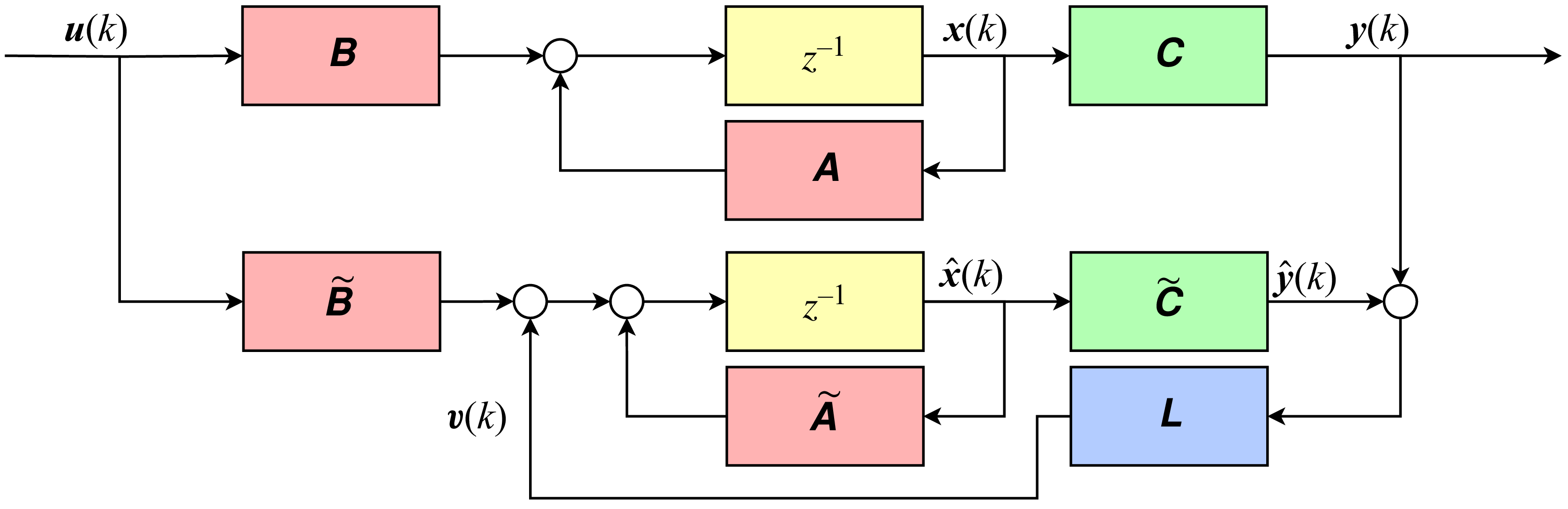
. The block diagram for this classic set-up is presented in figure 1, where
 $z^{-1}$
represents one time step delay with a notation that comes from the Z transform in the frequency domain. If the system is observable and
 $\unicode{x1D647}$
is designed (e.g. through pole placement) such that
 $\boldsymbol{x} - \hat {\boldsymbol{x}} \to 0$
as
 $k \to \infty$
, a perfect model (i.e.
 $\kern3pt \widetilde {\kern-3pt \unicode{x1D63C}} = \unicode{x1D63C}$
,
 $\kern3pt \widetilde {\kern-3pt \unicode{x1D63D}} = \unicode{x1D63D}$
and
 $\kern3pt \widetilde {\kern-3pt \unicode{x1D63E}} = \unicode{x1D63E}$
) would tendentially bring
 $\boldsymbol{v}[k]$
to zero and correction would no longer be needed.
Block diagram representing the discrete Luenberger observer for a linear dynamical system. The plant model is simulated in real time as the real system evolves. The correction signal
 $\boldsymbol{v}[k]$
is produced to rectify errors due to initial conditions, plant imperfections and unmodelled disturbances.

Another famous approach to estimators is the Kalman filter, which consists of an algorithm similar to the Luenberger observer. The main difference is that the estimator gain (here represented by
 $\unicode{x1D647}$
) is updated every time step according to the covariances related to process and measurement noises. The Kalman gain represents the optimal correction factor, assuming noise sources are Gaussian and white. Although the focus of the present work is to estimate states from limited sensor data without noise, we also present possible modifications to the NNO training to encompass measurement noise and insufficient sampling rate.
2.2. A nonlinear generalisation of the Luenberger observer
Consider the nonlinear dynamical system described by
 \begin{align} \boldsymbol{x}[k+1] &= \mathcal{F}(\boldsymbol{x}[k], \boldsymbol{u}[k]) , \\[-10pt] \nonumber \end{align}
 \begin{align} \boldsymbol{y}[k] &= \mathcal{C}(\boldsymbol{x}[k]) , \\[10pt] \nonumber \end{align}
where
 $\mathcal{F}(\boldsymbol{x}, \boldsymbol{u})$
is a general nonlinear function that governs the dynamics of the states and
 $\mathcal{C}(\boldsymbol{x})$
is a general nonlinear function that maps the states to the output variable space. If approximations
 $\widetilde {\mathcal{F}}(\boldsymbol{x}, \boldsymbol{u}) \approx \mathcal{F}(\boldsymbol{x}, \boldsymbol{u})$
and
 $\widetilde {\mathcal{C}}(\boldsymbol{x}, \boldsymbol{u}) \approx \mathcal{C}(\boldsymbol{x}, \boldsymbol{u})$
are available, an estimator loop can be built through the implementation of the difference equations
 \begin{align} \hat {\boldsymbol{x}}[k+1] &= \widetilde {\mathcal{F}}(\hat {\boldsymbol{x}}[k], \boldsymbol{u}[k]) + \boldsymbol{v}[k] , \\[-10pt] \nonumber \end{align}
 \begin{align} \boldsymbol{v}[k] &= \mathcal{L}(\boldsymbol{y}[k], \hat {\boldsymbol{y}}[k]) , \\[-10pt] \nonumber \end{align}
 \begin{align} \hat {\boldsymbol{y}}[k] &= \widetilde {\mathcal{C}}(\hat {\boldsymbol{x}}[k]). \\[10pt] \nonumber \end{align}
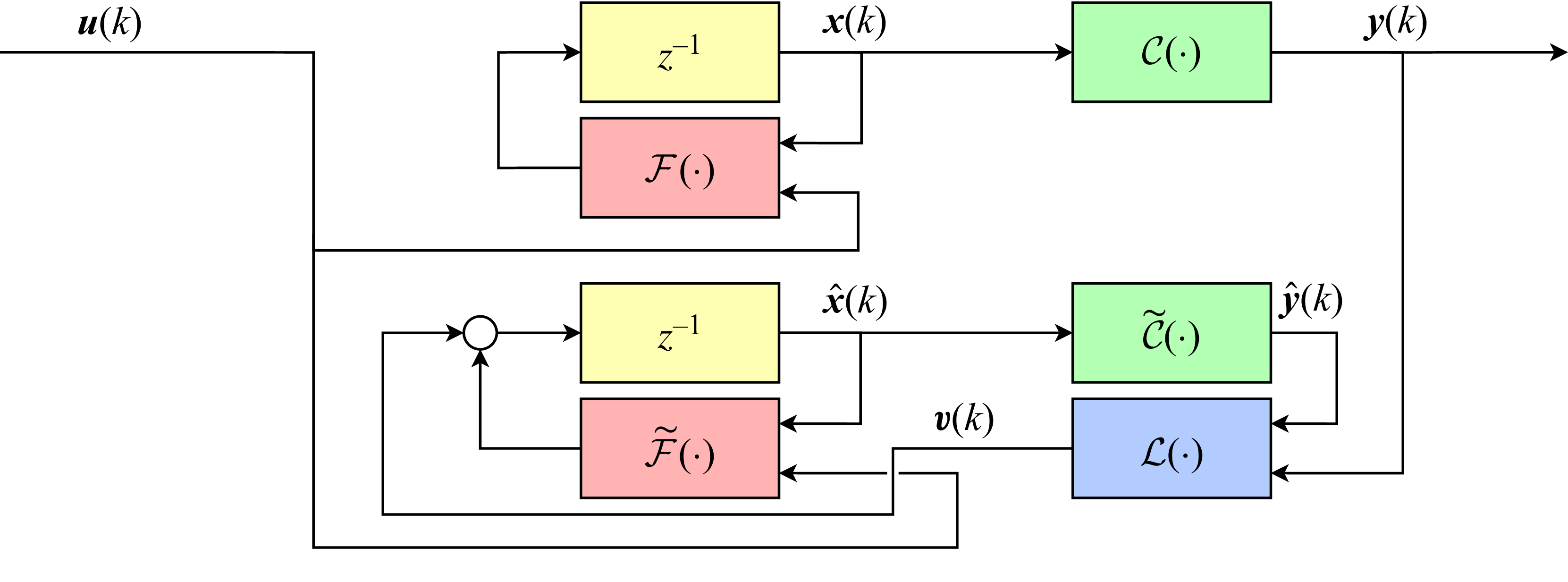
The structure is similar to the Luenberger approach, which can be verified by comparing the equations or by noticing the similarities between the block diagrams in figures 1 and 2. In both cases, the convergence of
 $\hat {\boldsymbol{x}}$
to
 $\boldsymbol{x}$
would also imply the convergence of
 $\hat {\boldsymbol{y}}$
to
 $\boldsymbol{y}$
and, since the trajectories for the estimated and actual states are constrained by the same dynamics (assuming the plant model is perfect),
 $\boldsymbol{v}[k]$
tends to zero and the estimation would be based only on predictions. In the present work the nonlinear operators
 $\widetilde {\mathcal{F}}$
,
 $\widetilde {\mathcal{C}}$
and
 $\mathcal{L}$
are implemented as NNs. Note that the process of computing
 $\boldsymbol{u}[k]$
is omitted, but it could be represented as
 \begin{align} \boldsymbol{u}[k] &= \boldsymbol{u}_{{c}}[k] + \boldsymbol{u}_{{o}}[k] , \\[-10pt] \nonumber \end{align}
 \begin{align} \boldsymbol{u}_{{c}}[k] &= \mathcal{K}(\hat {\boldsymbol{x}}) , \\[10pt] \nonumber \end{align}
where
 $\boldsymbol{u}_{{c}}[k]$
and
 $\boldsymbol{u}_{{o}}[k]$
are the closed-loop and open-loop components of the control input, respectively. The nonlinear function
 $\mathcal{K}$
is implemented as a NNC, and is not represented in figures 1 and 2 for simplicity. For more details on the controller, see Appendix A.
Block diagram representing a nonlinear generalisation of the discrete Luenberger observer. The colours are chosen to highlight the analogy with the classic approach for linear systems, depicted in figure 1.

2.3. Training set-up
The proposed observer loop consists of three main NNs: the NNSM
 $\widetilde {\mathcal{F}}$
, the output model
 $\widetilde {\mathcal{C}}$
and the NNO
 $\mathcal{L}$
. For closed-loop control cases, the loop will also contain the NNC
 $\mathcal{K}$
. To train the NNSM and the NNC, the methodology proposed by Déda et al. (Reference Déda, Wolf and Dawson2024) is followed; implementation details are provided in Appendix A. Thus, these models have already been trained and our objective is to train
 $\widetilde {\mathcal{C}}$
and
 $\mathcal{L}$
. All NNs involved in this work have a scaling layer to normalise their inputs such that the average and standard deviation of the data entering the first hidden layer are zero and one, respectively.
2.3.1. Output model
To train
 $\widetilde {\mathcal{C}}$
, a simple supervised learning approach is followed. First, let us consider numerical simulations, where all time-resolved system variables are available. In this case, one can simply collect
 $\boldsymbol{u}$
,
 $\boldsymbol{x}$
and
 $\boldsymbol{y}$
and find the best fit through backpropagation. The loss function chosen is
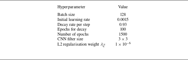
 \begin{align} l_{{\widetilde {\mathcal{C}}}} = \frac {1}{n_d} \sum _{i=1}^{n_d} \left \lVert \boldsymbol{y}_i - \widetilde {\mathcal{C}}(\boldsymbol{x}_i)\right \rVert _2^2 + \lambda _{\widetilde {\mathcal{C}}} \lVert \boldsymbol{w}_{\widetilde {\mathcal{C}}} \rVert _2^2 , \end{align}
where
 $\boldsymbol{w}_{\widetilde {\mathcal{C}}}$
are the weights of the output model,
 $\lambda _{\widetilde {\mathcal{C}}}$
tunes the strength of the L2 regularisation and
 $n_d$
is the number of samples in the input/output training batch.
For experimental applications, the training data for
 $\widetilde {\mathcal{C}}$
must be obtained through alternative means, as full state information is typically not available. One possible approach is to use models derived from equivalent numerical simulations to approximate
 $\mathcal{C}$
. However, it is important to note that transferring learned mappings between multi-source datasets (e.g. from simulations to experiments) is an ongoing challenge due inconsistent modelling assumptions and the lack of standardised coordinates and assessments (Fukami & Taira Reference Fukami and Taira2025). Such an approach would require careful validation, while potentially benefitting from robust feedback control and estimation systems. Alternatively, specialised sensors can be used to directly measure the system states during the training phase. These sensors are solely required for dataset collection and are not necessary for the observer loop after training. For instance, in the case of estimating velocity fields (states) from wall pressure measurements (outputs), PIV could be used to construct the training dataset by capturing the velocity field while simultaneously recording the wall pressure. Although challenging, simultaneous measurements are feasible with current technology, as demonstrated by Zigunov et al. (Reference Zigunov, Sellappan, Alvi, Ozawa, Saito, Nonomura and Asai2022b
). In this case, the data required for learning the static map
 $\widetilde {\mathcal{C}}$
does not need to be time-resolved at strict sample rates. Once trained, the network should be able to estimate velocity fields based only on wall pressure measurements, eliminating the need for PIV in real-time operation.
2.3.2. Neural network observer
Now that
 $\widetilde {\mathcal{C}}$
is trained, a closed-loop approach is proposed for training
 $\mathcal{L}$
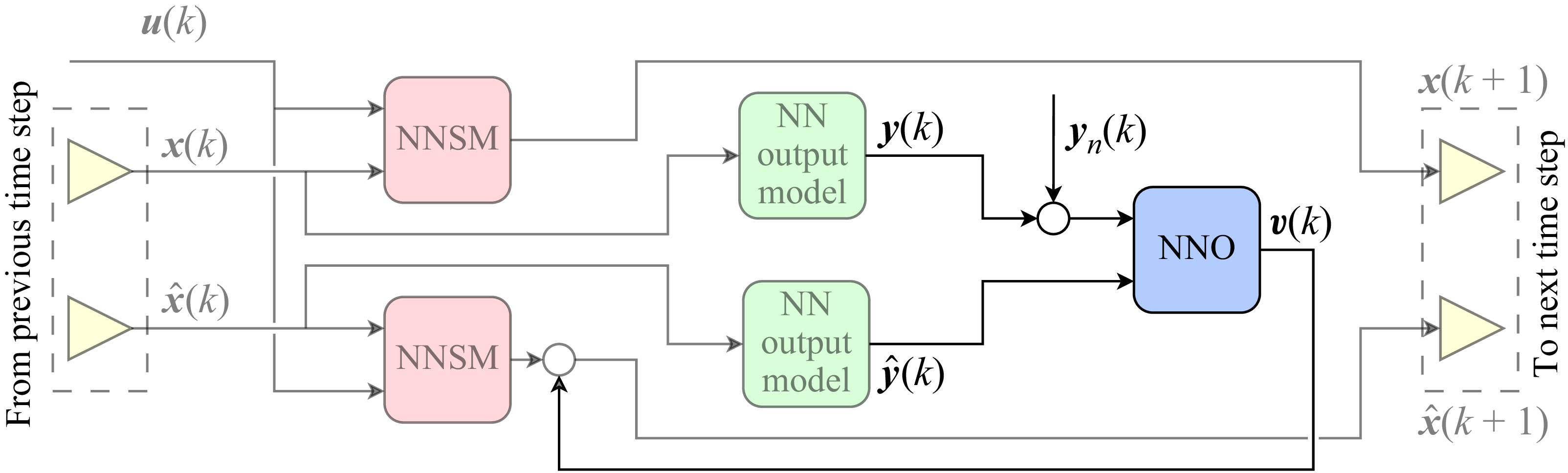
. The idea is to use a recurrent auxiliary configuration for training the NNO, in line with the method proposed by Yadaiah & Sowmya (Reference Yadaiah and Sowmya2006). This approach is analogous to the finite-horizon training strategies commonly found in closed-loop control literature (Bieker et al. Reference Bieker, Peitz, Brunton, Kutz and Dellnitz2020; Déda et al. Reference Déda, Wolf and Dawson2023). Figure 3 illustrates the structure of a single iteration of the observer loop, where
 $y_n$
is a measurement noise source, further detailed in this section. The colour scheme is consistent with that of figure 2, with analogous blocks highlighted similarly. The NNSM and the output model are each used twice during training: once to represent the real system (upper branch) and once to represent the observer predictor (lower branch). Their weights are kept fixed and only the weights of the NNO are updated. After training, the upper branch (representing the real system) is replaced by the actual plant during testing.
Schematic of a single iteration of the observer training loop. The NNSM and output model weights are frozen and only the NNO ones are updated. The hat notation (
 $\hat {x}$
and
 $\hat {y}$
) indicates estimated signals.

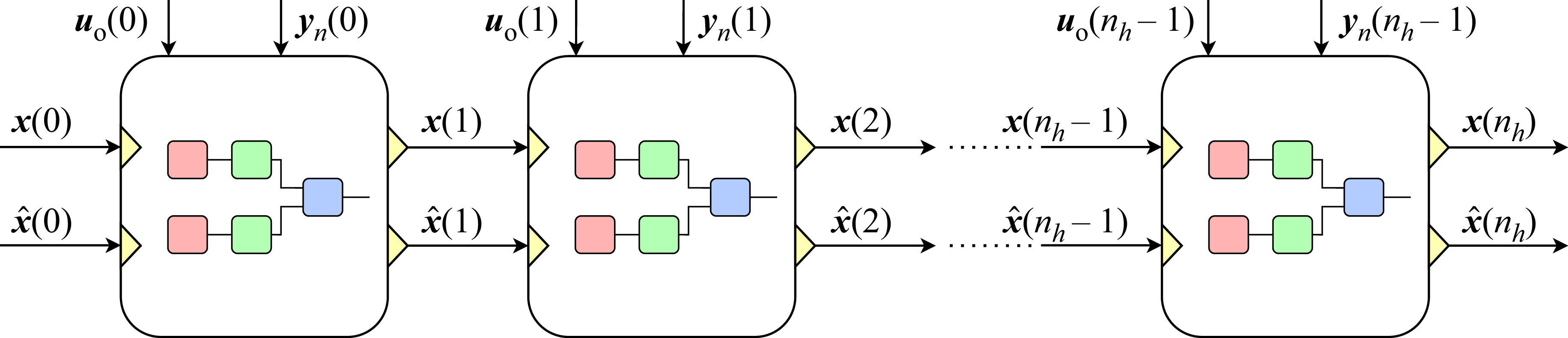
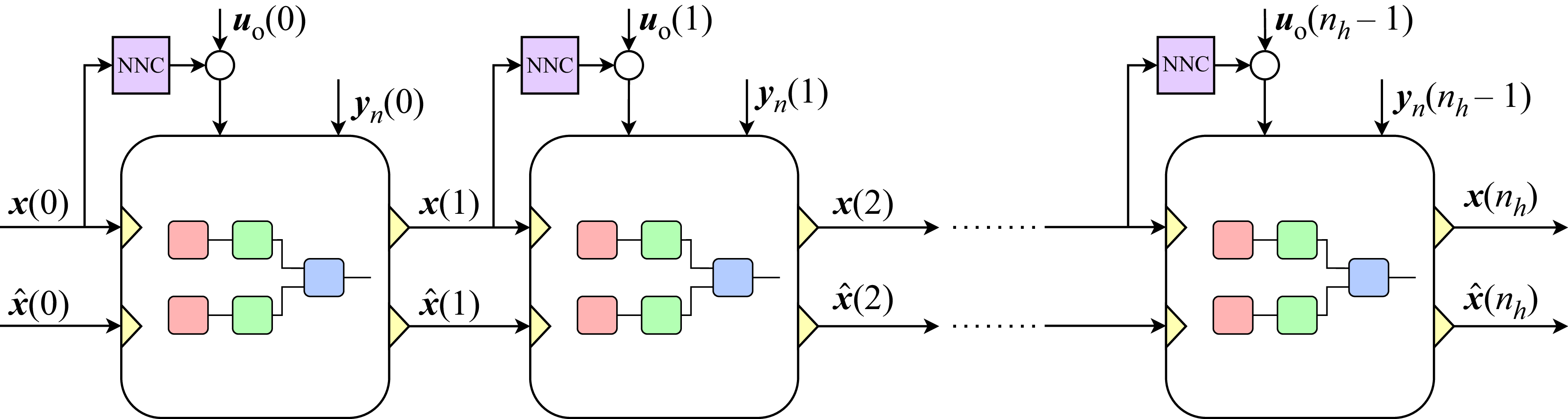
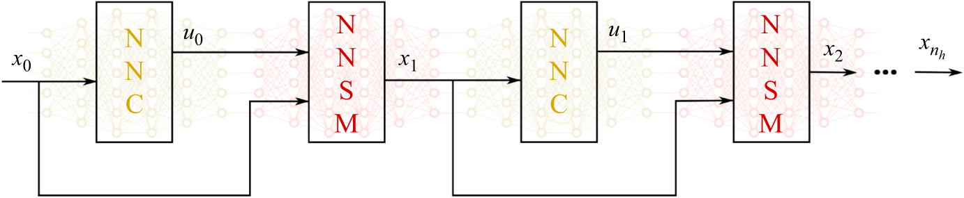
The single-step structure is unrolled along a finite horizon, as illustrated in figure 4, where
 $n_h$
denotes the horizon length. The training dataset includes initial conditions
 $\boldsymbol{x}[0]$
,
 $\boldsymbol{v}[0]$
and
 $\hat {\boldsymbol{x}}[0]$
, as well as open-loop input sequences of length
 $n_h$
:
 $\boldsymbol{u}_{{o}}[0], \boldsymbol{u}_{{o}}[1], \ldots , \boldsymbol{u}_{{o}}[n_h{-}1]$
. A measurement noise source
 $y_n[k]$
can be added to train the observer loop under conditions more reminiscent of those expected in real applications. If the measurement noise for a given application can be modelled (e.g. white or time-correlated Gaussian noise), that same type of noise can be employed during training. In the present work, two types of noise sources are employed: Gaussian white with zero mean and standard deviation
 $\sigma$
, and time-correlated noise obtained by filtering a white Gaussian noise source
 $y_n^*$
such that
 \begin{align} {y_n[k] = y_n^*[k] + \beta y_n[k-1]} , \end{align}
where
 $0 \leqslant \beta \leqslant 1$
determines the level of correlation in time. The filtered noise is then rescaled to match the original standard deviation
 $\sigma$
from the input white noise source.
Unrolled observer loop over a finite horizon of length
 $n_h$
, with each NN block representing the complete NNO loop.

Finite-horizon observer training loop with controller (NNC) inclusion.

The loss function used to train the NNO is the element-wise average of the expression
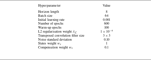
 \begin{align} l_{\mathcal{L}} &= \frac {1}{n_d n_h} \sum _{i=1}^{n_d} \sum _{k=1}^{n_h} \Big ( \big \lVert \boldsymbol{e}_{y,i}[k] \big \rVert _2^2 + \alpha _x \big \lVert \boldsymbol{e}_{x,i}[k] \big \rVert _2^2 + \alpha _v \big \lVert \boldsymbol{v}_i[k] \big \rVert _2^2 \Big ) + \lambda _{\mathcal{L}} \lVert \boldsymbol{w}_{\mathcal{L}} \rVert _2^2 , \\[-28pt] \nonumber \end{align}
 \begin{align} \boldsymbol{e}_y[k] &= \boldsymbol{y}[k] - \hat {\boldsymbol{y}}[k] , \\[-28pt] \nonumber \end{align}
 \begin{align} \boldsymbol{e}_x[k] &= \boldsymbol{x}[k] - \hat {\boldsymbol{x}}[k] , \\[0pt] \nonumber \end{align}
where
 $\alpha _x$
and
 $\alpha _v$
are coefficients that control the penalisation of state errors and correction signals, respectively, and
 $\lambda _{\mathcal{L}}$
controls the amount of L2 regularisation on the NNO weights
 $\boldsymbol{w}_{\mathcal{L}}$
. Index
 $i$
refer to the signals propagated from the
 $i$
th initial condition in the dataset. For training, the initial states
 $\boldsymbol{x}[0]$
are sampled from the true system (either numerical or experimental), and
 $\hat {\boldsymbol{x}}[0]$
uses the same values but shuffled to prevent the observer from always encountering the trivial solution
 $\boldsymbol{v}[k]=\boldsymbol{0}$
. The control signals used during training are random excerpts from those employed to generate the NNSM training data. Furthermore, figure 5 shows the inclusion of the NNC within the loop to ensure the observer is trained in state-space regions relevant to a closed-loop operation. In the present work, two different systems with control inputs are studied, namely a modified KS equation and a confined cylinder flow with jet actuation. In these cases, the training loop includes the NNC as shown in figure 5. On the other hand, for the third system studied, a turbulent boundary layer that does not involve closed-loop control, only open-loop signals (obtained from the dataset) are involved as depicted in figure 4.
Training the NNO can be challenging due to the potential for instability when operating in a closed loop. If
 $n_h$
is set too large, the feedback dynamics – especially with untrained, randomly initialised weights – may become unstable and result in exponential divergence. In practice, values such as
 $n_h = 15$
were found to be sufficient to cause training difficulties in some cases. To mitigate this, the horizon length
 $n_h$
is gradually increased over training: beginning from a small
 $n_h$
and incrementing it every few epochs. Both the initial
 $n_h$
and the increment schedule are treated as hyperparameters. The minimal required
 $n_h$
to make convergence possible primarily depends on the observer convergence time. The choice depends on the the coupled plant-observer dynamics, which is influenced by other hyperparameters. For example, higher noise levels
 $\sigma$
and correction penalisation
 $\alpha _v$
tend to make the NNO less aggressive, taking longer to converge and requiring a larger
 $n_h$
. A time-scale separation between estimation and control dynamics is desirable, with observer convergence being fast enough to mitigate estimation error interference on the control system. Therefore, BPTT for NNO training requires smaller horizons than NNCs for the same system. Further details are provided in Appendices A and B.
Another advantage of NNs as observers is the possibility of considering sensors with sampling rates lower than those required for control. By choosing an integer
 $\Delta k \gt 1$
, the training structure presented in figure 6 can be built. In this approach,
 $\boldsymbol{v}[k]$
is only computed every
 $\Delta k$
steps and propagated to all iterations until the next computation. Therefore, the lower sensor sampling time is taken into account during training. More information regarding the legacy NNSM and NNC utilised in this work, as well as training strategies and hyperparameters for the NNO and the NN output model are provided in Appendices A and B.
Training structure with time skips and
 $\Delta k = 3$
. Signal
 $\boldsymbol{v}[k]$
is propagated for time steps where measurements are absent.

3. Study cases
This section presents a description of the three systems analysed using the proposed methodology. We first test a modified KS equation to check the observer performance with a simple partial differential equation (§ 3.1). The task consists of estimating the complete velocity field using measurements from a reduced number of sensors. In this case, we introduce measurement noise and investigate training both with and without noise addition. The second problem studied consists of a confined cylinder flow with small jets used as actuators (§ 3.2). By reading signals from sensors located on the walls, the goal is to estimate the velocity values at a set of points along the flow field. For these two first cases, we leverage the estimated states to feedback stabilising NNCs, which should become possible, even though direct measurements are not available for the states vector. Finally, we test the approach with PIV data from a turbulent boundary layer experiment (§ 3.3). In this case, low-resolution noise-corrupted sensor data are employed to estimate the velocity fields along the boundary layer.
3.1. Modified KS equation
To test the proposed observation methodology, the partial differential equation known as the KS equation is chosen. It can be written as
 \begin{align} \frac {\partial \phi }{\partial t} + \phi \frac {\partial \phi }{\partial x_c} = -\frac {1}{R}\left ( P\frac {\partial ^2 \phi }{\partial x_c^2} +\frac {\partial ^4\phi }{\partial x_c^4}\right ) \! , \end{align}
where
 $R$
is equivalent to the Reynolds number in a fluid flow and
 $P$
represents a balance between energy production and dissipation. The values
 $R=0.25$
and
 $P=0.05$
are chosen, which are the same ones studied by Fabbiane et al. (Reference Fabbiane, Semeraro, Bagheri and Henningson2014), who showed that convective instabilities are present for certain wavenumbers. The spatial coordinate is represented by
 $x_c$
. The dynamical system solved in this work is a modified version of the KS equation that adds control inputs to actively access the states, besides including a term to ensure that a single uniform natural equilibrium configuration exists. It can be written as
 \begin{align} \frac {\partial \phi }{\partial t} + \phi \frac {\partial \phi }{\partial x_c} = -\frac {1}{R}\left ( P\frac {\partial ^2 \phi }{\partial x_c^2} +\frac {\partial ^4\phi }{\partial x_c^4}\right ) -\frac {Q}{L} \int _{0}^{L}(\phi (x_c)-V)\,\text{d}x_c + \sum _{i=0}^m B_i(x_c) u_i. \end{align}
The term
 $-Q/L \int _{0}^{L}(\phi (x_c)-V)\,\text{d}x_c$
ensures that, for
 $u(t) = 0$
,
 $\phi (x_c) = V$
is the only possible uniform natural equilibrium possible. We choose
 $Q=0.0005$
,
 $V=0.2$
and
 $L=60$
, where
 $L$
is the domain length. A positive value of
 $Q$
renders the uniform mode (wavenumber zero) stable, while a negative value would make the solution grow indefinitely. For
 $Q=0$
, an infinite number of uniform equilibrium solutions would be found. Furthermore, the domain length
 $L$
is chosen to be large enough such that unstable modes related with lower wavenumbers are present. The vector
 $\boldsymbol{u}$
is composed of
 $m=3$
control inputs
 $u_i$
that modulate the amplitude of three evenly spaced Gaussian windows
 $B_i$
along the spatial domain. The control signals are modulated by Gaussian windows with standard deviation
 $\sigma _B=0.4$
, the same value employed by Fabbiane et al. (Reference Fabbiane, Semeraro, Bagheri and Henningson2014). We employ three actuators in order to test the methodology in a scenario with more than one actuator, while keeping the number low enough to avoid significant overlaps between the actuation windows.
The system is spatially discretised by explicit fourth-order centred finite difference schemes with
 $\Delta x_c = 1$
and periodic boundary conditions (BCs). These BCs allows for continuous feedback of convectively unstable waves, rendering the dynamic system globally unstable. Evolution in time is performed along a time window described in Appendix B for data gathering, using the standard fourth-order Runge–Kutta scheme with
 $\Delta t = 0.025$
, ensuring numerical stability. Control and estimation are conducted at
 $\Delta t_c=400\boldsymbol{\cdot }\Delta t = 10$
, the same sampling time of the trained NNSMs, such that
 $t=k\Delta t_c$
, where
 $t$
and
 $k$
are the continuous and discrete-time variables, respectively. Following control theory notation, the discrete time is represented by natural numbers. From the signals
 $\phi (x_c)$
at the 60 points that compose
 $\boldsymbol{x} = [\, \phi (0), \ldots , \phi (59) \,]^T$
, we choose
 $n_s$
evenly distributed ones to compose the sensors vector
 $\boldsymbol{y}$
. Figure 7 presents the discretised states, outputs and actuation schemes, showing examples where different numbers of sensors are used, whose positions are represented by the red circles. In this work we present results of several study cases with this implementation of the modified KS equation, including tests with either 15 or 3 sensors. We also add white or time-correlated Gaussian measurement noise in some cases, as well as sensing with
 $\Delta k \gt 1$
.
State, sensor and actuation scheme for discretised KS equation. The black dots represent each of the 60 state positions. The sensor locations are highlighted with red circles for the cases with 15 (a) and 3 (b) sensors. The coloured dots show the Gaussian actuation profiles.

The nonlinear operators
 $\widetilde {\mathcal F}(\boldsymbol{\cdot })$
,
 $\widetilde {\mathcal C}(\boldsymbol{\cdot })$
,
 ${\mathcal K}(\boldsymbol{\cdot })$
and
 ${\mathcal L}(\boldsymbol{\cdot })$
are implemented as NNs with fully connected hidden layers. The NNSM
 $\widetilde {\mathcal F}$
and the NNC
 $\mathcal K$
are the same as those trained by Déda et al. (Reference Déda, Wolf and Dawson2024). At the beginning of the simulation for data sampling, the initial condition
 $\phi (x_c)=V$
is chosen.
3.2. Confined cylinder flow
In the present work a confined cylinder flow is also investigated. The set-up is implemented in Nek5000 (Li & Zhang Reference Li and Zhang2022) for a Reynolds number
 ${Re} = 150$
, based on the cylinder diameter
 $D$
and the average inlet velocity. At such conditions, the flow is globally unstable, presenting periodic vortex shedding. The upper and lower channel walls are spaced
 $H=4D$
apart, with the cylinder centred in between,
 $4D$
away from the inflow and
 $20D$
away from the outflow. The grid and geometry are presented in figure 8. The simulations are performed using a time step
 $\Delta t = 5.0\times 10^{-3}$
along the time windows described in Appendix B for gathering training data, while sampling for control and estimation is performed at
 $\Delta t_c=40\boldsymbol{\cdot }\Delta t = 2\times 10^{-1}$
. Again,
 $t=k\Delta t_c$
, where
 $t$
and
 $k$
are the continuous and discrete-time variables, respectively.
Confined cylinder flow domain and computational grid.

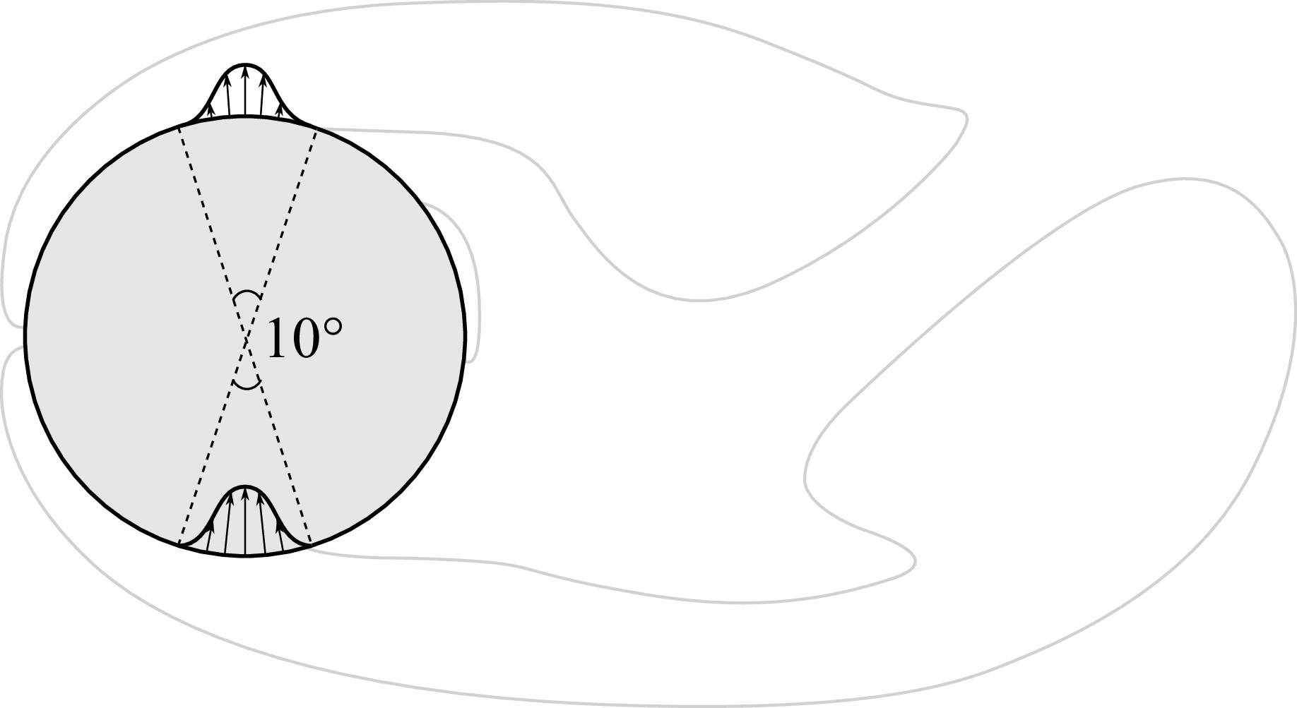
To actively modify the flow, minijets are implemented in phase opposition as Dirichlet BCs, providing a zero-net mass flux. The control input
 $\boldsymbol{u}=Q^*=Q/Q_{\textit{ref}}$
consists of a single entry: the normalised injected mass flow rate at a single minijet, where
 \begin{align} Q_{\textit{ref}} = \int _{-D/2}^{D/2}\phi _\rho \phi _u\,\text{d}y . \end{align}
Here,
 $\phi _\rho =1$
is the density of the incompressible flow and
 $\phi _u = 6(H/2-y)(H/2+y)/H^2$
is the horizontal component of velocity at the inflow, which is a parabolic profile. A cosine window function along the angular coordinate (coincident with the cylinder centre) sets the profile presented in figure 9, such that the maximum absolute values take place at the bottom-most and top-most points of the cylinder wall. The actuation effort is limited to
 $|Q^*|\lt 0.06$
.
Actuation scheme applied to the cylinder flow. Blowing/suction jets in opposition are modulated by a single control input.

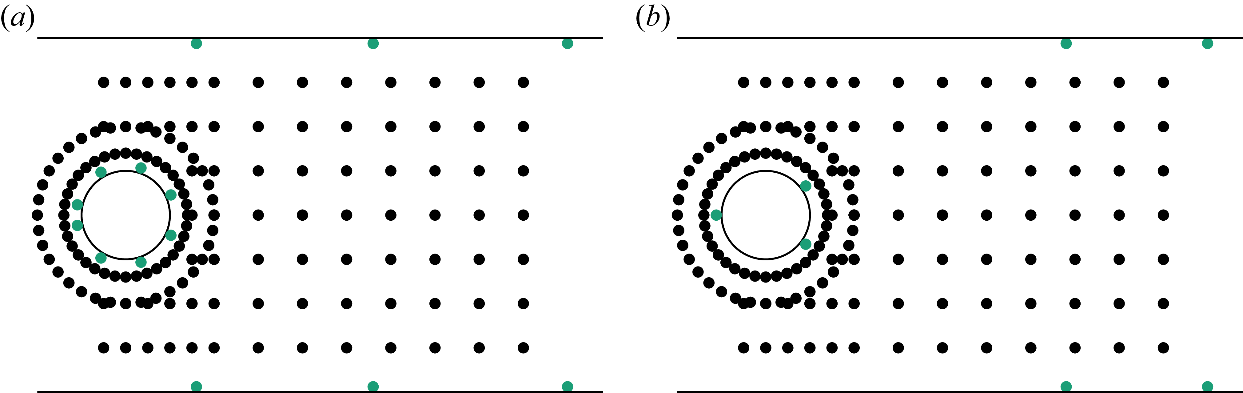
The vector
 $\boldsymbol{x}$
(featuring 306 states) is composed of the horizontal and vertical velocities
 $\phi _u$
and
 $\phi _v$
, respectively, at 153 locations marked with black dots in figure 10. This is the same set-up previously studied by Rabault et al. (Reference Rabault, Kuchta, Jensen, Réglade and Cerardi2019), and the state feedback NNC proposed by Déda et al. (Reference Déda, Wolf and Dawson2024) successfully stabilised this flow configuration. In the present work we assume that measurements of
 $\boldsymbol{x}$
are unavailable, proposing more realistic sensor set-ups to compute estimates
 $\boldsymbol{\hat {x}}$
, which in turn are fed to the NNC. Here, pressure measurements
 $\phi _p$
are probed on the wall, at locations marked with green dots in figure 10. The sensors are distributed at the cylinder and channel walls. Configurations with sensors exclusively at the cylinder walls are avoided, since the estimator loop would have to rely on a very accurate NNSM to correctly propagate waves downstream. In closed-loop control systems, this is often not desirable, since real-world applications involve uncertainties that include plant variations (e.g. inflow velocity variations) and unsensed/unmodelled perturbations. Clearly, this makes the closed-loop control of the open cylinder flow an even more challenging task, since measuring variables away from the wall presents practical challenges. Moreover, the open cylinder flow at an equivalent Reynolds number presents a longer wake recirculation, meaning that important features are farther from the cylinder wall while closed-loop control is hindered due to significant delays between actuation inputs and downstream variables.
Probing set-ups for the confined cylinder flow, featuring (a) 14 and (b) 7 sensor locations. The state vector
 $\boldsymbol{x}$
consists of horizontal and vertical velocity components at locations indicated by black dots. The measurement vector
 $\boldsymbol{y}$
consists of pressure measurements taken at locations marked with green dots near the cylinder and channel walls.

Two set-ups are analysed, where either 14 or 7 sensors are used to compose
 $\boldsymbol{y}$
. Here, the nonlinear operators
 $\widetilde {\mathcal F}(\boldsymbol{\cdot })$
,
 $\widetilde {\mathcal C}(\boldsymbol{\cdot })$
,
 ${\mathcal K}(\boldsymbol{\cdot })$
and
 ${\mathcal L}(\boldsymbol{\cdot })$
are also implemented as NNs with fully connected hidden layers. The NNSM
 $\widetilde {\mathcal F}$
and the NNC
 $\mathcal K$
are also provided by Déda et al. (Reference Déda, Wolf and Dawson2024) (see Appendix A).
Experimental set-up of the slanted cylinder flow. Time-resolved PIV images of a turbulent boundary layer are captured within the cyan window.

Mean horizontal velocity contour (a), mean horizontal velocity curves (b) and Reynolds stresses (c) along the original window coordinates. Coordinates are presented in boundary layer thickness units.

3.3. Turbulent boundary layer
The last problem analysed consists of a turbulent boundary layer developing over a bullet-shaped body with a slanted cut. The experimental set-up used in this study was originally proposed by Zigunov (Reference Zigunov2020), who collected the PIV data used for the present NN estimation trials. The set-up is shown in figure 11, where
 $\phi _u$
and
 $\phi _v$
velocity components are captured within the cyan window. The experiment is performed at Reynolds number
 ${Re} = 40\,000$
relative to diameter
 $D= \mathrm{146.05\, mm}$
of the cylinder section. The free-stream velocity is 4.1 ms−1 and the vectors are sampled at 5000 frames per second. The dataset provided for the current NN trainings were post processed, providing 1999 snapshots, including the velocity components
 $\phi _u$
and
 $\phi _v$
, as well as pressure, obtained via the one-shot omnidirectional pressure integration (OS-MODI) through matrix inversion (Zigunov & Charonko Reference Zigunov and Charonko2024). From the 45.66
 $\times$
29.0 mm window shown in figure 11, a quadrilateral region is selected, where the velocity vectors are more accurate. The region is depicted in figure 12(a), where the coloured region plus the dark area represent the cyan window from figure 11. The coloured region contains the relevant data, and this specific figure presents the mean horizontal velocity. Figures 12(b) and 12(c) show the velocity profile and the Reynolds stresses (respectively) that characterise the flow, both averaged along time and the horizontal axis. The wall is located at y = 5.45 mm and the average boundary layer thickness is
 $\delta = 9.25\,\mathrm{mm}$
, based on 99 % of the free-stream velocity. This corresponds to half of the middle section of the PIV window. The data cover a time period corresponding to 177 convective time units based on the boundary layer thickness and the free-stream velocity.
Snapshots depicting contours of
 $\phi _v$
along the boundary layer. Each frame is 10 time steps apart from their neighbour. The PIV-sampled image is shown in row (a), where the window used to compose
 $\boldsymbol{x}$
and the probe locations (green dots) chosen for the problem are highlighted. The vertical green line shows the region where the BCs
 $\boldsymbol{u}$
are imposed in the model. The
 $\phi _v$
components of
 $\boldsymbol{x}$
(states) and
 $\boldsymbol{y}$
(probed values) are depicted in rows (b) and (c), respectively.

Figure 13(a) presents contours of
 $\phi _v$
at snapshots spaced 10 time steps apart, so that the convection of structures can be clearly noticed. It encompasses a cropped region containing only the relevant area where information is present. To compose the states vector
 $\boldsymbol{x}$
, we use the smaller window indicated in the the figure, resulting in two images containing
 $128\times 64$
pixels each, one for
 $\phi _u$
and one for
 $\phi _v$
– the latter being depicted in figure 13(b) – totalling
 $128\times64\times2 = 16\,384$
states. At the measured location, the boundary layer is turbulent due to a bypass transition from tripping implemented in the experiment; the source of disturbances is not contained within the data. This brings a relevant issue when modelling the flow dynamics, as it is not possible to predict the next time step without having information from upstream. To solve this issue, we use the control inputs vector
 $\boldsymbol{u}$
to represent the BCs, which are treated as forcing. This source term is composed by 32 values of
 $\phi _u$
plus 32 of
 $\phi _v$
probed at the green line shown in figure 13(a), where measurements at every second pixel are taken, totalling
 $64$
entries for
 $\boldsymbol{u}$
. Although this is not a realistic approach for real-world applications since it would require real-time measurements in many locations away from the walls, it is a workaround to test the NNO capabilities when dealing with complex turbulent flows. In real applications, the region encompassing the states could include the position where the disturbances arise, and therefore, such forcing modelling would not be required. Alternatively, hotwire sensors could be implemented to measure flow velocities away from the wall, combined with other types of NN architectures, such as graph neural networks (GNNs), which do not require regular grids like the CNNs. Moreover, in § 4.3 we show that the NNO deployment is able to provide estimations with acceptable accuracy loss even when the information is omitted.
Finally, to compose the outputs vector
 $\boldsymbol{y}$
, we employ
 $\phi _u$
and
 $\phi _v$
values at the
 $4\times 8$
array green dots shown in figure 13(a), totalling 64 variables. Figure 13(c) presents the resulting low-resolution image built from the readings at these sensor locations. We also add an artificial white Gaussian noise source
 $\boldsymbol{y_n}$
to the normalised measurements, with standard deviation
 $\sigma =0.1$
.
3.3.1. Neural network implementations for NNO loop
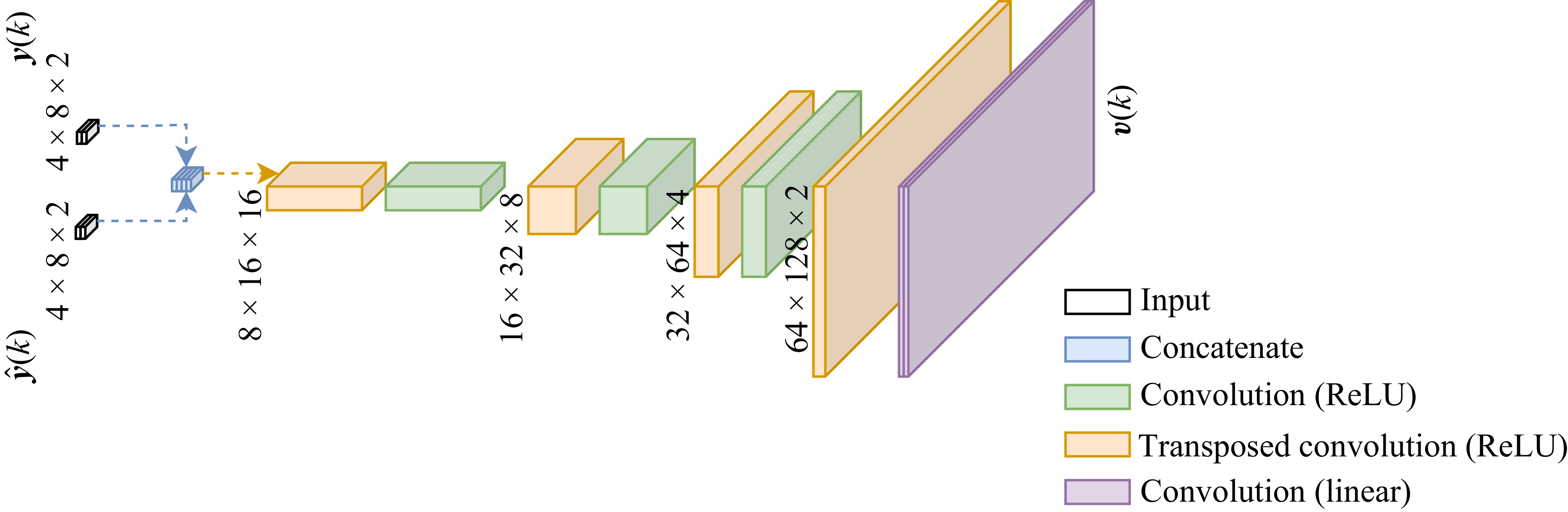
A specialised NN architecture is developed to process the high number of states. As presented in figure 14,
 $\phi _u$
and
 $\phi _v$
are concatenated to form a two-channel image. The same is done to
 $\boldsymbol{u}$
, which is upscaled through a nearest-neighbour algorithm. The states and BCs are combined to take advantage of the spatial relations between them. Pure convolutions are applied in succession, such that pixels are updated only based on their neighbours. By avoiding fully connected layers, we also take better advantage of the limited dataset size, since each pixel of
 $\boldsymbol{x}$
can be seen as a data unit that goes through the same nonlinear function. At the output, the resulting image is sliced so the initial size is recovered. Each component
 $\phi _u$
and
 $\phi _v$
is normalised separately so that their values range from zero to one. This normalisation process is performed for all the networks trained, and the input (
 $\boldsymbol{u}$
) and output (
 $\boldsymbol{y}$
) vectors are slices of these normalised variables.
The architecture for the output model is shown in figure 15. Here, the input states are downscaled through convolution and max pooling steps. The outputs correspond to the low-resolution images shown in figure 13(c). Although this network could be implemented as a simple slicing function – thus, not requiring trainable parameters – we implement it as a nonlinear function to avoid the assumption that
 $\mathcal{C}(\boldsymbol{x})$
is known. Finally, the NNO architecture is presented in figure 16, where the correction signal
 $\boldsymbol{v}[k]$
consists of the two-channel output image, which is summed to the corresponding predicted state images. More training details including hyperparameters are provided in Appendix C.
Neural network architecture used for the turbulent boundary layer NNSM. Here ReLU activation is used, except for the output convolution layers, which are linear.

Neural network architecture used for the turbulent boundary layer NN output model. Here ReLU activation is used, except for the output layer, which is linear.

Neural network architecture used for the turbulent boundary layer NNO. Here ReLU activation is used, except for the last fully connected layer, which is linear.

Several limitations of the proposed methodological approach should be noted. The sensors used are limited to the plane where variables were sampled during the experiments, which can hinder turbulence modelling given its three-dimensional nature, particularly considering the absence of a third velocity component (
 $\phi _w$
) in the dataset. Furthermore, since the proposed experiment was not configured for active control and considering that our group lacks experimental resources to reproduce the proposed experiment, the deployment of the NNOs is limited to open-loop tests, where control input signals adopt the role of the aforementioned BCs contained within data, propagated along time through the NNSM, whose predictions are rectified by the observer.
During the development of the present work, different CNN architectures were tested, one of which included specialised treatment of the lower border with independent convolutional filters. Such treatment of wall BCs may present limitations due to the wall not being present in the data images, which means that the lower border presents non-zero velocity components, as shown previously in figure 12. Since such treatment did not yield noticeable improvements, the simpler version described in the present section is chosen, with the same set of filters being applied to the entire spatial window, thus fewer parameters are required. A U-net architecture was also investigated with different numbers of downscaling steps for the NNSM, but no improvements to model performance were observed. Therefore, we chose the simpler architecture shown in figure 14 with a reduced parameter count.
3.3.2. Baseline methods
To illustrate the advantage of implementing the proposed estimation topology over the reconstruction of
 $\boldsymbol{x}$
from
 $\boldsymbol{y}$
through direct NN inference, we also train a NN super-resolution model to upscale the low-resolution images into the original states. The architecture employed is similar to that presented for the NNO (see figure 16) for a fair comparison. The difference is that the
 $\hat {\boldsymbol{y}}$
input to the NNO and the concatenation layer are skipped, since there is no dynamic model of the flow to leverage predictions. Additionally, the super-resolution NN outputs the reconstructed states
 $\boldsymbol{x}$
directly instead of
 $\boldsymbol{v}$
. The NNO and the super-resolution NN are trained to estimate the states in the presence of white Gaussian noise with
 $\sigma = 0.1$
, which is artificially added to the normalised values of
 $\phi _u$
and
 $\phi _v$
. Although the experimental data are already contaminated with unknown measurement noise, we further add the artificial source to better test the NNO ability to work under non-ideal conditions. This noise level, as well as the spatial grid of
 $4 \times 8$
points are chosen for operations where the super-resolution approach fails to provide accurate reconstructions. This allows for assessing the proposed NNO technique under challenging conditions.
Since the study is conducted for a small spatial window, the problem is dominated by convection, although some distortions are seen in the flow structures being transported. Due to these characteristics, we also implement a convective baseline model, which is built by assuming a frozen-field (FF) hypothesis. We take the BCs vector
 $\boldsymbol{u}$
and apply the transport equations
 \begin{align} \frac {\partial \phi _u}{\partial t} &= -\bar {\phi }_u(x,y)\frac {\partial \phi _u}{\partial x} , \\[-10pt] \nonumber \end{align}
 \begin{align} \frac {\partial \phi _v}{\partial t} &= -\bar {\phi }_u(x,y)\frac {\partial \phi _v}{\partial x} , \\[10pt] \nonumber \end{align}
where the mean horizontal flow velocity
 $\bar {\phi }_u(x,y)$
is computed at each pixel. The spatial discretisation is performed through a first-order backward finite difference scheme and time integration is conducted using the fourth-order Runge–Kutta scheme. To ensure numerical stability, the time step is reduced to one fifth of the original
 $\Delta t$
at which data was sampled, although the results are only shown at the time instants that match the experiment. Since the BCs have half the resolution of the final image columns, we simply replicate each pixel when upscaling.
The super-resolution NN provides reconstructions directly from the sampled
 $\boldsymbol{y}[k] +\boldsymbol{y}_n[k]$
, while the FF model propagates the BCs as a dynamic model. Each of these approaches are compared with the NNO approach proposed, which combines model predictions with corrections by leveraging the
 $\boldsymbol{y}[k] +\boldsymbol{y}_n[k]$
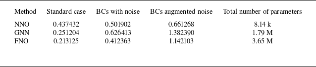
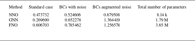
measurements. Furthermore, we also compare the NNO with state-of-the-art techniques, namely a GNN model and a Fourier neural operator (FNO), which are presented in Appendix D. Direct comparisons between model architecture and observer topology are not perfect. In fact, the FF model, as well as the GNN and the FNO models could be implemented as surrogate models
 $\widetilde {\mathcal{F}}$
in the structure presented in figure 2. The tests, however, bring a focus on the benefits of combining a very simple NNSM (with a significantly smaller number of parameters than the GNN and FNO) with sensor data, even in unideal conditions.
4. Results
In this section, results are presented for study cases where trained NNOs are deployed in a closed loop, as illustrated in figure 17. For the KS equation and the cylinder flow, the nonlinear plant is a numerical simulator, which is run to produce the results presented in the current section. For these cases, we present both open-loop (for illustrative purposes) and closed-loop control results. For open-loop tests, the system is perturbed using staircase signals as control inputs (
 $\boldsymbol{u}=\boldsymbol{u}_{{o}}$
). For closed-loop control, the stabilising NNC is incorporated into the loop, fed solely by the estimated states, i.e.
 $\boldsymbol{u}=\boldsymbol{u}_{{c}}=\mathcal{K}(\hat {\boldsymbol{x}})$
. The states vector
 $\boldsymbol x$
are internal to the nonlinear plant, and therefore unknown to the control/observer loops. The initial condition shown in the results comes from the open-loop perturbed systems, corresponding to the sweep stage described in Appendix A.
Block diagram representing the nonlinear observer in the closed loop to estimate flow states. The control input can be toggled between open loop and closed loop. The nonlinear plant returns
 $\boldsymbol{y}[k]$
as a function of
 $\boldsymbol{u}[k]$
and its internal states.

For the experimental boundary layer set-up, only legacy data from prior experiments are available. We only conduct open-loop trials by using the control inputs (
 $\phi _u$
and
 $\phi _v$
BCs) provided in the dataset. Therefore, the nonlinear plant is reduced to accessing the dataset at each time step. The loop structure, however, is still the same shown in figure 17, but
 $\boldsymbol{u}[k]$
always receives the prescribed input signal
 $\boldsymbol{u}_{{o}}[k]$
without any subsequent adjustment for closed-loop control. The initial condition
 $\hat {\boldsymbol x}[0]$
consists of two images containing mean flow data.
4.1. Modified KS equation
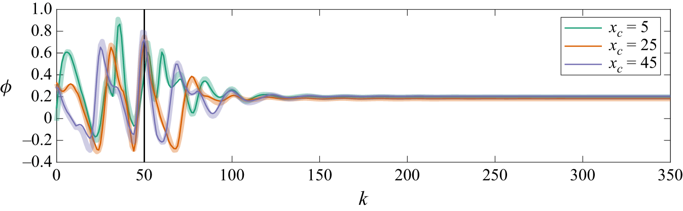
Results of seven KS simulations are shown following the set-up described in § 3.1. A time window of 350 time steps of the simulation are presented, where state tracking under open-loop perturbations is presented for
 $0\leqslant k\lt 50$
and with closed-loop control for
 $50\leqslant k\lt 350$
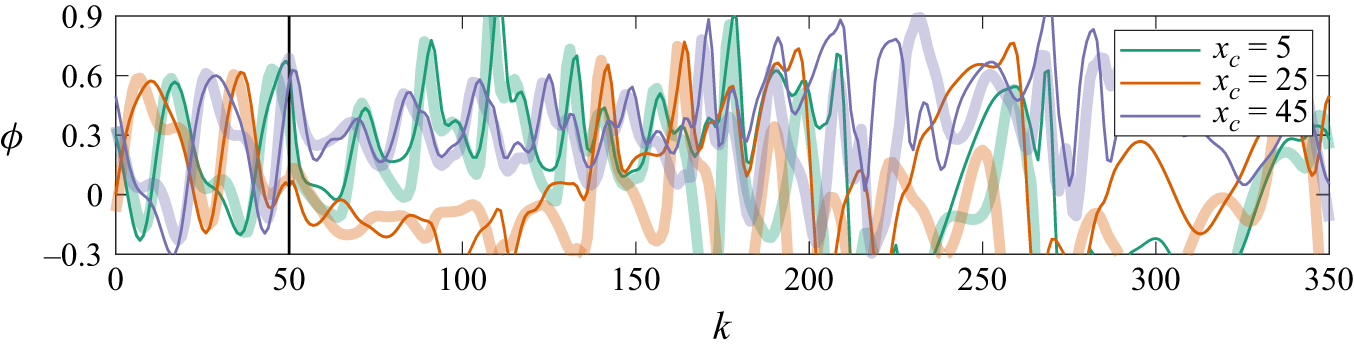
. We choose to present the last 350 steps, showing a part of the solution that continued from the chaotic attractor; therefore, the initial growth from equilibrium is omitted. Figure 18 shows results when 15 sensors are used. The estimated
 $\phi$
values are presented at coordinates
 $x_c=2$
,
 $x_c=22$
and
 $x_c=42$
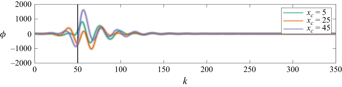
, where no sensors are present, and therefore, states are harder to estimate as they depend more on model predictions along time. Similarly, figure 19 shows results with only three sensors, also at coordinates without sensors. The comparison of the estimated states (thin opaque lines) with the actual states (thicker transparent lines), show that the tracking is almost perfect, with a slight difference in the case with fewer sensors. When closed-loop control is turned on, the system is properly stabilised through feedback of the estimated states, with estimation remaining accurate as the system stabilises. These first two cases presented, with sets of either 3 or 15 ideal sensors, produce control responses that are very close to those found by Déda et al. (Reference Déda, Wolf and Dawson2024), who used ideal state feedback. This is expected since the state estimation is very accurate and the same NNC is used.
Results with 15 sensors for state estimation and feedback control of the modified KS equation. Three states are shown comparing the estimated states
 $\hat {\boldsymbol{x}}$
(thin opaque lines) and the actual states
 $\boldsymbol{x}$
(thick transparent lines), at specific locations
 $x_c$
. Closed-loop control is first applied at
 $k=50$
, as indicated by the vertical black line.

As in figure 18, but with three sensors.

Results with 15 sensors and white Gaussian noise with
 $\sigma = 0.03$
for the modified KS equation. Three states are shown at locations
 $x_c$
where sensors are present for comparing the estimated states
 $\hat {\boldsymbol{x}}$
(thin opaque lines) and the actual states
 $\boldsymbol{x}$
(thick transparent lines). The thin transparent lines show the measured signals with noise
 $y+y_n$
.

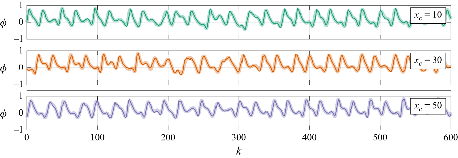
Results with added noise are shown in figure 20 for the set-up with 15 sensors, at locations where sensors are present. By choosing such locations, it is possible to directly compare the measured signals with the corresponding states. This is done similarly for all cases with unideal sensing (either due to noise or with
 $\Delta k \gt 1$
). Here, the measurement is contaminated with white Gaussian noise with standard deviation
 $\sigma =0.03$
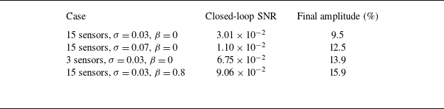
. In this case, states are shown at locations where sensors are present, so a comparison between the actual states and the measured signals (thin transparent lines) can be established. During the open-loop stage, an average signal-to-noise ratio (SNR) of approximately
 $3.72\times 10^{0}$
is observed. As the system is controlled, the states oscillations are reduced, lowering the average SNR to around
 $3.01\times 10^{-2}$
. With such low SNR, the observer is not able to estimate the states correctly and a new range of oscillation amplitude is reached, at which further attenuations are unlikely to occur. In this situation, the controller is not able to bring states to steady state, but the oscillation amplitudes are reduced to 9.5 % of the original amplitude of the uncontrolled system (measured through the square root of the ratio between SNRs). With
 $\sigma =0.07$
(see figure 21), an average open-loop SNR of
 $7.13\times 10^{-1}$
is found. The controller reduces oscillation amplitudes to 12.5 %, after which an SNR close to
 $1.10\times 10^{-2}$
is seen. From the plots, it can be noticed that the estimated signals are typically closer to the actual states than the directly measured noise-corrupted signals (thin transparent lines).
As in figure 20, but with
 $\sigma =0.07$
.

With only three sensors and
 $\sigma = 0.03$
(see figure 22), we can also preserve the ability to perform closed-loop control. An amplitude attenuation to
 $13.9\,\%$
is seen for the actual states, after which the average SNR is measured at
 $6.75\times 10^{-2}$
. This greater value shows that fewer sensors are worse at observing states under noisy conditions. At the same SNR levels, the other case studies were still able to estimate states with sufficient accuracy to further attenuate oscillations.
As in figure 20, but with three sensors.

The proposed technique also allows for training with different types of noise. Figure 23 shows a case where time-correlated noise with
 $\sigma = 0.03$
and
 $\beta =0.8$
(as defined in (2.14)) is added, both during training and deployment. In this example, using time-correlated noise made attenuation worse, but the NNC is still able to reduce oscillations to around 15.9 % of the original amplitudes, at an average SNR of
 $9.06\times 10^{-2}$
. Since the proposed time-correlated noise presents slower variations along time, it is possible that improved attenuation could be achieved with larger
 $n_h$
during training. However, filtering with
 $\beta =0.8$
introduces a power spectral density shift from higher frequencies to lower ones, as the filtered signal is scaled to match the standard deviation of the original white noise. In the KS equation, higher frequencies (associated with higher wavenumbers) are dynamically attenuated (Fabbiane et al. Reference Fabbiane, Semeraro, Bagheri and Henningson2014). As a result, the more relevant lower frequencies, to which the KS equation is more sensitive, become stronger. This provides a possible explanation for the more limited attenuation observed when time-correlated noise is applied. We note that the frequency-wise sensitivity to noise depends on the coupled plant-controller-observer system, and a systematic sensitivity characterisation is beyond the scope of the present work. The attenuation values reported here are summarised in table 1.
Results for each KS case with measurement noise. The final amplitude is measured as the percentage of the uncontrolled oscillation amplitude.

As in figure 20, but with time-correlated noise with
 $\beta =0.8$
.

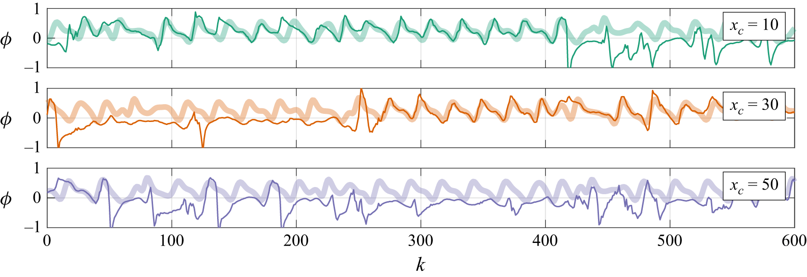
Results with 15 sensors and measurements with
 $\Delta k = 8$
for the modified KS equation. Estimated states
 $\hat {\boldsymbol{x}}$
(thin opaque lines) and the actual states
 $\boldsymbol{x}$
(thick transparent lines) are shown. The staircase signal represents the sensor measurements at a lower sampling rate.

The last two KS cases investigated utilise 15 sensors with either
 $\Delta k=8$
or
 $\Delta k=16$
, i.e. measurements are only sampled every 8 or 16 time steps of the NNSM/NNC. Thus, for most of the time, the same values
 $v[k=N\Delta k]$
(where
 $N \in \mathbb{N}$
) are used to correct the NNSM predictions until the next measurement update at
 $k=(N+1)\boldsymbol{\cdot }\Delta k$
. With
 $\Delta k = 8$
(see figure 24), the tracking is nearly perfect, rendering the NNC able to correctly stabilise the plant. In figure 25, however, we see that
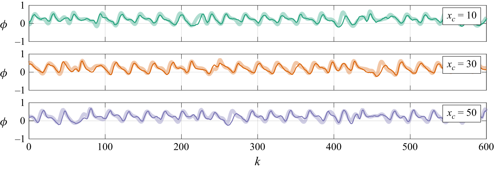
 $\Delta k = 16$
is enough to prohibit stabilisation with the available NNSM. The maximum
 $\Delta k$
value is probably related to the model ability to produce good predictions for longer, without the need for corrections via sensor information. Therefore, in situations where the output sample periods are shorter than the time scales of the error, we should expect the estimation to work well, even with
 $\Delta k \gt 1$
. Supplementary movie 1, available at https://doi.org/10.1017/jfm.2026.11464, summarises the time response comparing all cases. Other cases are analysed in Appendix E, where a configuration with stronger nonlinearities is considered for comparing the nonlinear NNO with linear approaches, and Appendix F, where the use of an EKF is compared with the present methodology.
As in figure 24, but with
 $\Delta k = 16$
.

4.2. Confined cylinder flow
The validation of closed-loop stabilisation of the cylinder flow introduced in § 3.2 is presented here, where the NNO estimates relevant flow variables by reading limited sensor information. Results are shown with actuation performed in two stages: under open-loop perturbations for
 $0\leqslant k\lt 200$
and with closed-loop control for
 $200\leqslant k\lt 500$
.
Results of the case with 14 sensors are presented in figure 26, which shows
 $\phi _u$
and
 $\phi _v$
at a few selected points, marked with different colours along the cylinder wake and upstream of the cylinder. The initial conditions are close to the equilibrium point and the flow develops to near the limit cycle after a few time steps, before the controller is turned on. Estimated states are shown as thin opaque lines, with the same colours used to represent their respective points in space. By comparing them with the actual states, represented by thicker transparent lines, it is possible to verify that the main tendencies are well captured, especially at the lower shedding frequency that matches lift oscillations. In general, we observe that signals with twice the shedding frequency, related to drag oscillations, are harder to track precisely. This is illustrated by looking at
 $\phi _u$
in the yellow point, situated at the channel centreline. During the closed-loop stage, the NNO is capable of providing estimations with enough accuracy to enable proper NNC performance. Indeed, only very small oscillations are seen after the main transient, as vortex shedding is almost completely suppressed. The results with 14 sensors are very close to those obtained by Déda et al. (Reference Déda, Wolf and Dawson2024) through direct state feedback (assuming states are known), albeit slight differences in the settling time occur due to an imperfect estimation of states.
Results for state estimation and control of the confined cylinder flow with 14 sensors. State curves are shown with the same colours as the respective coloured point locations. Thin opaque and thick transparent lines show estimated and real states, respectively. Closed-loop control is applied at
 $k=200$
, as indicated by the vertical black lines.

For the case study with seven sensors shown in figure 27, state estimates during the open-loop stage are able to follow the tendencies of the actual states. The same behaviour is seen during the closed-loop control stage, where the NNC is able to significantly attenuate vortex shedding. However, after reaching state-space regions close to the natural equilibrium point, high-frequency oscillations are introduced by closed-loop dynamics, which makes the NNC respond with small perturbations that hinder convergence. To illustrate the difference between results with different numbers of sensors, figure 28 presents
 $\phi _v$
contours for the uncontrolled flow, as well as the final snapshot for each controlled case. The levels presented are sufficiently saturated such that small oscillations can be visualised. In both controlled cases, the flow gets considerably closer to the equilibrium point in comparison with the uncontrolled flow, but weaker wake oscillations still propagate, which is more prominent in the case with fewer sensors. Supplementary movie 2 plots
 $\phi _v$
contours evolving with time for each case.
As in figure 26, but with seven sensors.

Vertical velocity
 $\phi _v$
fields at
 $k=499$
(last snapshot) for (a) the uncontrolled flow, (b) the controlled flow with 14 sensors, and (c) the controlled flow with 7 sensors.

4.3. Turbulent boundary layer
The NNs depicted in figures 14, 15 and 16 are trained by using the first 1500 snapshots (from a total of 1999) from the experimental boundary layer dataset. The same procedure is applied for the super-resolution NN mentioned in § 3.3, which is used to compare the results with the proposed estimator methodology.
Flow snapshots are presented in figures 29 and 30, where contours show the fluctuations
 $\phi _u'$
and
 $\phi _v'$
around the mean flow obtained from the original dataset. The images are measurements from
 $k=1780$
to
 $k=1788$
, skipping every odd frame, evolving from left to right. For both figures, row (a) presents the original PIV data, while row (b) presents a downscaled solution, built by selecting pixel values at the proposed sensor locations. The latter is shown before the addition of measurement noise
 $\boldsymbol{y}_n$
. The temporal evolution of the NNSM is shown in row (c), where only the initial conditions
 $\boldsymbol{x}[k=0]$
are provided and states are obtained iteratively through
 $\boldsymbol{x}[k+1]=\widetilde {\mathcal{F}}(\boldsymbol{x}[k])$
. Noticeably, the model tends to smoothen smaller structures, but is able to reproduce the convective characteristics of the flow. Also, for time instants shown, which are far from the initial condition, it is possible to observe that the average flow is shifted, and the deviation can be seen as mismatching colours occurring in the top-right corner of the images in row (c) for
 $\phi _u'$
. This leads to relatively high estimation errors, as will be further discussed. This mean flow offset, which arises after a few time steps from the original condition, could be related with long-term inaccuracies as the BCs are propagated. One way to possibly attenuate this issue is by increasing the model sampling time by skipping samples during training. By doing so, cumulative errors due to successive autoregressive evaluations could be diminished.
Contours of
 $\phi _u'$
from
 $k=1780$
(leftmost) to
 $k=1788$
(rightmost), skipping the odd frames. The rows show (a) the original data, (b) the low-resolution sensor data before adding the noise source, (c) the NNSM evolution, (d) the FF model evolution, (e) the direct reconstruction from noisy sensor data, and (f) the NNO estimation using the NNSM and noisy sensor data. These results are also illustrated in more detail in movie 3.

The FF flow evolution is shown in row (d), and as discussed below, the errors seen are smaller than those found for the NNSM, at least provided ideal BCs. We choose the NNSM instead of the FF model for training the NNO to avoid an a priori assumption of the plant characteristics, as well as to show that a certain level of robustness to model imperfections can be expected of the NNO closed-loop estimation. This is a desirable feature, since in real-world control systems plant variations are expected, and a closed-loop controller/observer can often compensate for such variations.
The results of direct reconstructions from noisy sensor data inputs are presented in row (e) of figures 29 and 30. The super-resolution NN, trained with a structure similar to the NNO – although without the
 $\hat {\boldsymbol{y}}$
inputs – is presented here to show the advantages of leveraging sensor data for state estimation. The contours show that the noisy measurements make the reconstruction prone to temporal instability, which can be observed by the intermittent structures that quickly appear and disappear. This is expected since the direct reconstruction saves no memory from past estimations. On the other hand, NNO results illustrated in row (f) provide the smallest error values with improved temporal stability, which is achieved by leveraging both the noisy measurement data and the imperfect NNSM. The evolution of the estimated states through the NNSM, i.e. the prediction step, saves information from previous estimations, thus allowing for rejecting part of the noise introduced to sensors. The noisy low-resolution images, in turn, can be used to reduce errors caused by imperfect predictions, such as strong smoothening and the mean flow offsets. For rows (c), (d) and (f),
 $\boldsymbol{x}[k=0]=\bar {\phi }_u(x,y)$
is used. For better visualisation of each case, supplementary movie 3 shows the comparison for the entire time series for
 $\phi _u'$
and
 $\phi _v'$
.
As in figure 29, but for
 $\phi _v'$
.

Comparison between the errors of the flow estimation methods shown in figures 29 and 30. Only data to the left of the vertical dashed line is used for training.

Velocities
 $\phi _u$
and
 $\phi _v$
computed at halfway up the PIV window height and at 94 % of the distance between the inflow and the outflow.

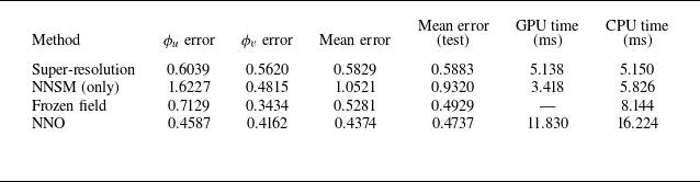
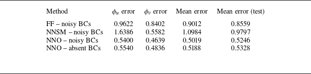
To compare results for each case, we propose the squared error metric normalised by the velocity fluctuations
 \begin{align} e_{\phi _u} [k] &= \frac {\|\phi _u[k] - \hat {\phi }_u[k]\|^2}{\|\phi _u[k]-\bar {\phi }_u(x,y)\|^2} , \\[-10pt] \nonumber \end{align}
 \begin{align} e_{\phi _v} [k] &= \frac {\|\phi _v[k] - \hat {\phi }_v[k]\|^2}{\|\phi _v[k]-\bar {\phi }_v(x,y)\|^2} , \\[10pt] \nonumber \end{align}
where the norms are computed by flattening the images. The horizontal and vertical velocity components of the estimated states are represented as
 $\hat {\phi }_u$
and
 $\hat {\phi }_v$
, respectively. The errors along time are presented in figure 31. The NNSM case uses only the model to propagate the BCs, while the super-resolution NN directly reconstructs the velocity fields from noisy sensor data. While the former presents higher error values (particularly for
 $\phi _u$
), the super-resolution NN presents rapid oscillations due to measurement noise. By combining both sensor data and the model, the NNO loop is able to achieve better temporal stability and smaller errors, comparable to the FF model, with the advantage of leveraging output feedback to enable increased robustness in real-world applications, an important characteristic for closed-loop control strategies. Figure 32 presents
 $\phi _u$
and
 $\phi _v$
predictions in the range
 $k=1000$
to
 $k=1400$
, measured at half the PIV window height and at 94 % of the streamwise distance between inflow and outflow. For this probe located near the outflow boundary of the spatial domain, the
 $\phi _u$
signal reconstructed by the NNSM exhibits a displacement relative to the original flow signal. In addition, both
 $\phi _u$
and
 $\phi _v$
obtained from the NNSM display a slight phase shift. The super-resolution approach, in turn, yields compromised results due to the noisy input data. The FF model is able to reproduce part of the original fluctuations but overly smooths both
 $\phi _u$
and
 $\phi _v$
. The most accurate reconstruction is provided by the NNO, which successfully captures the majority of oscillations in both velocity components. For
 $\phi _v$
, the peaks and phases of the oscillations are resolved with higher fidelity, while for
 $\phi _u$
, the agreement is less precise, but still satisfactory. Although results are not perfect, we must emphasise that this is a convection-dominated problem and small structures may pass through the flow window without being sensed by probes.
Table 2 summarises the errors, which are averaged in time to obtain a single quantity. The average is computed starting from
 $k=1500$
, corresponding to the interval for which the BCs were not seen in training. The inference time is also presented for each case. All methods are evaluated on both a central processing unit (CPU, Intel®
 $\textrm {Core}^{\textrm {TM}}$
i7-7820X @ 3.60 GHz) and a graphics processing unit (GPU, NVIDIA RTX 2070 Super). The FF model is evaluated on CPU only and, since each iteration of time integration is executed five times to match the original data sampling time as explained in § 3.3.2, the evaluation time presented is the combined time of the five iterations. While the NNO presents the lowest error, it only represents a reduction of 6 %, which could, at first sight, suggest that the higher evaluation time might not justify the proposed methodology. However, it is important to emphasise that the direct propagation of BCs without corrections through sensor feedback could lack robustness when operating beyond ideal conditions. To verify this assumption, we additionally test the performance of the estimation/reconstruction systems when random white noise is added with a standard deviation of 0.18 to the normalised
 $\boldsymbol{u}$
vector containing the flow BCs.
Time-averaged errors for different methods. The mean error is the average of
 $\phi _u$
and
 $\phi _v$
errors over all time steps. The test interval comprises errors starting from
 $k=1500$
. Evaluation time per iteration is also shown. For the NNO, the total inference time for the three involved NNs are shown.

Figure 33(a) shows the results in terms of error for the FF case. The curves show that the model provides considerably larger errors when the signal is contaminated with noise, especially for predictions of
 $\phi _v$
. Figure 33(b) shows the same curves for the NNSM, which shows more subtle error differences. Here, we use the same NNSM trained without adding noise to
 $\boldsymbol{u}$
in order to remain faithful to the methodology proposed. This means that there could be room for improvement if a noise source with similar characteristics were introduced during training to make the models more robust. The ability to reject noise also reflects in lower error variations for the NNO loop, whose results are shown in figure 33(c), also exhibiting resilience in the presence of noise while keeping smaller error values by leveraging sensor data. Finally, figure 33(d) presents the results for a case where the BCs are unseen by the NNO loop. In this case, the mean flow
 $\bar {\phi }_u(x=0,y)$
is fed to the NNSM in the NNO loop at every time step. The error increases only marginally and mostly affects the inflow region, as shown in figures 34 and 35. There, the velocity fluctuation contours for absent and noise-corrupted BCs are shown with the pixel-wise squared difference. Here, instead of showing every consecutive time step, we show a sequence at
 $k=590$
,
 $k=600$
and
 $k=610$
. As large-scale structures enter the domain, more intense errors are seen at the left border when no BCs are provided. In the last snapshot, when the structure is already within the domain and reaches the sensors, the error is reduced along this region. Without the BCs, the NNSM and the FF model are unable to work alone, since no structure is present on the inlet to be transported with the flow. Therefore, no comparison is relevant in these cases. The time-averaged errors for the cases with noise or without BCs are summarised in table 3. The above results are also illustrated in supplementary movie 4. Moreover, further robustness tests are provided in Appendix D, where accurate surrogate models implemented as a GNN and a FNO are subject to noisy BCs without sensor feedback for comparison.
Errors before and after the contamination of the inlet BCs signals with white noise.

5. Conclusions
We develop and apply a machine learning framework for online sensor-based state estimation using dynamic surrogate models of a given plant. The proposed method estimates unsteady flow variables under limited sensing conditions. Unlike conventional approaches that directly reconstruct flow states from sparse measurements, our formulation is inspired by control theory, combining prediction and correction steps. In this context, machine learning serves as a means to extend classical linear approaches, specifically the Luenberger observer in combination with full state feedback control. The proposed methodology is tested with three dynamical systems including a modified KS equation, a confined cylinder flow and a turbulent boundary layer. The two first cases are investigated using numerical simulation models and include flow estimation and closed-loop control, while the third case employs experimental data from PIV measurements and only considers flow estimation.
Contours of
 $\phi _u'$
(coloured) for
 $k=590$
,
 $600$
and
 $610$
with respective squared differences (grey scale). The rows show the (a) original data, (b) the FF model evolution, (c) the NNSM evolution, (d) the NNO estimation with BCs. Noisy BCs are imposed in (b), (c) and (d), while row (e) shows the NNO estimation without BCs.

As in figure 34, but for
 $\phi _v'$
.

The study conducted on the controlled KS equation serves as a proof of concept of the methodology capability to estimate states of discretised partial differential equations. By measuring only a subset of the state space, we demonstrate that the states can be accurately estimated, even in the presence of different types of noise and with coarse sampling intervals. The estimations enable closed-loop control via full state feedback using a NNC, allowing for wave attenuation up to the point where measurement noise dominates the output signals. In contrast to an EKF, which requires variable gain updates based on initial error statistics, the optimal estimator obtained through training does not incorporate a variable gain and provides solutions based on the state/output relationships observed during training. The Kalman filter requires an estimate of the initial error covariance to iteratively compute a gain that converges according to measurement noise statistics. In contrast, our approach is trained without any prior knowledge of initial condition errors and its performance is evaluated solely based on the current estimated and measured outputs. Moreover, the proposed NNO approach does not require local linearisations, as it is trained with the nonlinear models in the loop.
Time-averaged errors for different methods with noisy or absent BCs. The mean error (test) is computed only for snapshots starting from
 $k=1500$
.

To assess the performance of the proposed NNO in an actual flow problem, we demonstrate its ability to estimate a discretised velocity field in the flow past a cylinder immersed in a plane channel. In this case, 306 state variables, corresponding to the velocity components along the cylinder wake, are estimated using pressure sensors located on the cylinder surface and the channel walls. For both configurations tested, employing either 14 or 7 sensors, the estimated states enabled closed-loop control that attenuated vortex shedding. Although the stabilising NNC did not fully suppress the instabilities, it achieved a substantial reduction in oscillation amplitudes without requiring retraining of the NNC. The use of only a few wall-mounted pressure sensors highlights the potential of this approach for experimental applications, where direct velocity measurements in regions away from the walls are difficult to obtain.
Aiming to bridge the gap between simulations and experiments in the field of flow control, we additionally tested the training approach with legacy data provided from PIV of a turbulent boundary layer. By implementing specialised architectures for each of the involved NNs, we achieve promising results, demonstrating that, in specific regions of the state space, it is feasible to estimate the main flow features from low-resolution, noise-corrupted experimental data. Furthermore, we show that combining such data with an NNSM enhances the estimation accuracy compared with employing either strategy individually, while also providing a degree of robustness to unforeseen phenomena, such as noisy BCs implemented as control inputs. Since formal guarantees are not provided given the generality and black-box nature of the proposed NNO framework, the robustness is assessed empirically to demonstrate confidence in the approach. We note that the concerted effort to include empirical results, however, does not fully replace theoretical guarantees. The turbulent flow under consideration is high order and inherently complex, making precise estimation of all flow variables challenging, if not impossible. For certain problems, such as flows exhibiting periodic vortex shedding, the presence of dominant modes facilitates the inference of flow states from a limited set of measurements. However, in control applications, perturbations can reveal stable modes that remain unobserved under unforced conditions.
For problems similar to the present boundary layer, sparse sensor data can lead to ambiguous representations of the size and shape of turbulent structures, and smaller scales may remain unresolved due to low-resolution measurements. Future experimental campaigns, which are beyond the scope of the present work, could assess the performance of feedback control systems driven by such imprecise state estimates. Additional possibilities include the application of the proposed NNO–NNC framework to these experimental settings. This will require the development of models with improved parameter efficiency to enable real-time evaluation, allowing for model embedding into a field programmable gate array system or to a microcontroller. As presented in Appendix D, architectures with low parameter counts when compared with state-of-the-art machine learning approaches are still able to present robust estimations when built around the proposed methodology. For application in embedded systems, where hardware presents significant limitations, simpler NNs can be advantageous. It may also be necessary to develop models encompassing all NNs employed in the current approach, potentially incorporating observers with internal memory to represent states in a latent space, thereby enabling dynamic output feedback. Another important step for practical deployments is the thorough quantification of uncertainties. While the present work achieved promising performance in terms of robust flow estimations, future investigations also include the characterisation of aleatoric and epistemic uncertainties, which can be key for applications in extrapolative scenarios.
While the present work did not provide a systematic approach for sensor placement, such an important step in the observer design also remains open for future work. Approaches such as model training via input L1 regularisation and sensitivity analyses for quantification of dominant directions in the measurements are possible approaches that can leverage the availability of machine-learning-based models.
Supplementary movies
Supplementary movies are available at https://doi.org/10.1017/jfm.2026.11464.
Acknowledgements
We thank Dr F. Zigunov (Syracuse University) for providing the experimental data and important technical information regarding the boundary layer experiment. We also thank Dr F. Scarano (TU Delft) and Dr M. Choudhari (NASA Langley Research Center) for their foundational insights that made this work possible.
Funding
The authors acknowledge the financial support received from Fundação de Amparo à Pesquisa do Estado de São Paulo, FAPESP, under Grants Nos. 2013/08293-7, 2021/06448-0 and 2024/21444-9, and from Conselho Nacional de Desenvolvimento Científico e Tecnológico, CNPq, under Grants Nos. 304320/2024-2 and 444329/2024-2. Financial support from Universidade Estadual de Campinas, through FAEPEX Grant No. 2375/24, is also acknowledged. STMD acknowledges support from the US National Science Foundation award #2238770.
Declaration of interests
The authors report no conflict of interest.
Data availability statement
The data and software that support the findings of this study will be openly available in the repository (https://github.com/las-unicamp) after the review process.
Author contributions
T.D.: conceptualisation, methodology, software, validation, investigation, data curation, writing, visualisation. B.R.: methodology, software, validation, writing. W.W.: conceptualisation, methodology, writing, supervision, project administration, funding acquisition. S.D.: conceptualisation, methodology, writing, supervision.
Appendix A. Details on legacy NNs
The NNSM and NNC employed for the KS and cylinder flow cases studied in this work were trained a priori, and the implementation details are reported by Déda et al. (Reference Déda, Wolf and Dawson2024). To train both NNs, the solver is perturbed with an open-loop signal
 $\boldsymbol{u}_{{o}}$
(sweep stage) and the states
 $\boldsymbol{x}$
are sampled. The open-loop signal consists of a random staircase signal, inspired by square-wave forcing for approximating linear systems by exciting multiple frequencies. With a staircase signal, we avoid toggling between only two fixed forcing amplitudes and produce richer data for nonlinear dynamics modelling.
Using the Adam optimiser, the NNSM
 $\widetilde {\mathcal{F}}$
is trained first to approximate
 \begin{align} \boldsymbol{x}[k+1] \approx \widetilde {F}(\boldsymbol{x}[k],\boldsymbol{u}[k]) . \end{align}
The model is then linearised through backpropagation and an iterative method is employed to search for a natural equilibrium solution:
 \begin{align} \boldsymbol{x}^* = \widetilde {F}(\boldsymbol{x}^*,0) . \end{align}
The NNC
 $\mathcal{K}$
is then trained using BPTT, where initial conditions from the dataset obtained in the sweep stage are propagated in a closed loop along a finite horizon (similarly to what is done for the NNO in the current paper). This propagation leverages NN recurrency only at the training stage as shown in figure 36. Here,
 $\mathcal{K}$
(the NNC model) is tuned to minimise a loss function that balances the time-averaged squared error
 $\left \lVert \boldsymbol{x}-\boldsymbol{x}^*\right \rVert ^2$
and control inputs
 $\left \lVert \boldsymbol{u}\right \rVert ^2$
. By bringing states closer to a natural equilibrium point within the training horizon, this loss function is chosen to indirectly obtain a stabilising controller. The solver is then executed along an unforced release stage (
 $\boldsymbol{u}[k] =0$
), followed by a control stage, where the closed-loop signal
 $\boldsymbol{u}[k] = \mathcal{K}(\boldsymbol{x}[k])$
is employed. The process is repeated for a number of iterations, but since an NNC is now available, the sweep stage incorporates the closed-loop signal such that
 $\boldsymbol{u}[k] = \boldsymbol{u}_{{o}}[k]+\mathcal{K}(\boldsymbol{x}[k])$
. This new data allows for retraining the NNSM and the NNC with points closer to equilibrium, improving the model accuracy near this region. The training hyperparameters described here are shown in table 4.
Number of time steps and training horizon length for the KS and cylinder cases.

The NNC training schematic. A recurrent model is built for training only. Only the NNC weights are updated to bring the propagated states
 $\boldsymbol{x}_1$
,
 $\boldsymbol{x}_2$
,
 $\ldots$
,
 $\boldsymbol{x}_{n_h}$
closer to the equilibrium point.

The main structure of the NNSMs consists of fully connected layers, preceded by a direct transfer layer, whose weights are penalised using L1 regularisation to eliminate some of the input states from the calculations. Figure 37 illustrates this architecture. For the NNC, the structure is similar, but the direct transfer layer is comprised of zeros (at the same locations where zeros are present at the respective trained NNSM) and ones (otherwise). Table 5 presents the final number of states that are not excluded in each case, as well as the number of layers and nodes to summarise the complexity of the NNs. For further training details, we refer the reader to the original article (Déda et al. Reference Déda, Wolf and Dawson2024).
Details of the NNC and NNSM used for the KS and cylinder flow cases.

Schematic of the NNSM where the red (blue) nodes are related to weights penalised by the L2 (L1) regularisation. A ReLU function is employed in the nodes with a white mark, while a linear function is used for the other nodes.

Appendix B. Neural network observer details
The NN output models and NNOs trained for the KS and cylinder flow cases are simply composed of fully connected layers. Their hyperparameters are summarised in table 6. For the cylinder case, the dataset was split in batches. The horizon length used to compute the NNO loss function started with
 $n_h = 5$
for both cases, being incremented by one every 300 epochs from the 600th epoch for the KS case, and for every 200 epochs from the 200th epoch in the cylinder flow, being capped at the vales shown in the table. Adam optimisation is chosen, with the learning rates specified in the table.
Hyperparameters of the NN output model and NNO.

The data for training the NN output model and the NNO are obtained by applying open-loop control perturbations to the solvers, starting from initial conditions close to the equilibrium points of the system. For the KS cases, the initial conditions are set as
 $\phi (x_c)=V$
, while for the cylinder, equilibrium is reached by letting the NNC stabilise the flow, providing an initial condition. The perturbations are first applied with the pre-trained NNC turned on, assuming full state feedback, since the NNO is not trained yet, configuring a combined open-loop/closed-loop stage (OL + CL). With the stabilising controller turned on, the perturbations allow for sweeping the state space near the equilibrium point. After that, a stage with only open-loop perturbations is applied to produce data in a broader region of the state space (OL). Finally, the last stage is run with closed-loop control without the open-loop perturbations (CL). The number of time steps for each stage is also shown in table 6.
Appendix C. Neural networks of boundary layer case
To ensure a better long-term prediction capability of the boundary layer NNSM presented in figure 14, we train the network weights by unrolling the model response in time within a finite horizon
 $n_{h\mathrm{s}}$
. From the initial dataset containing the initial states
 $\unicode{x1D653}_0$
for training, we compute
 $\widetilde {\unicode{x1D653}}_i = \widetilde {\mathcal{F}}(\widetilde {\unicode{x1D653}}_{i-1})$
aiming to minimise the element-wise average of the loss expression
 \begin{align} l_{\widetilde {\mathcal{F}}} = \sum _{i=1}^{n_{d\mathrm{s}}}\sum _{k=1}^{n_{h\mathrm{s}}} \big(\unicode{x1D653}_k - \widetilde {\unicode{x1D653}}_k \big) , \end{align}
where
 $n_{d\mathrm{s}}$
is the batch number of samples and
 $\unicode{x1D653}_k$
comes from the experiment. During training, a linear warm-up is applied, where the learning rate grows linearly from 0 to 0.001 during 50 epochs. Table 7 summarises the hyperparameters for the NNSM.
Hyperparameters of the turbulent boundary layer NNSM.

For the output model, the learning rate modulation is performed via discrete decay only. The hyperparameters are shown in table 8. Finally, the hyperparameters used for the NNO are shown in table 9. Similarly to the NNSM, a linear warm-up profile and a discrete exponential decay is applied here.
Hyperparameters of the turbulent boundary layer output model.

Hyperparameters of the turbulent boundary layer NNO.

Appendix D. Comparison with GNNs and FNOs
In this appendix we put our NNO implementation for the boundary layer case in perspective with more sophisticated surrogate models, namely a GNN model and an FNO model. Direct comparisons between the NNO and the proposed state-of-the-art approaches are limited since the NNO leverages external information provided by sensors, not relying on pure predictions. In principle, sophisticated models such as FNOs and GNNs could be utilised with the proposed NNO framework, and therefore, the methodologies are not mutually exclusive. In § 4.3 we leveraged a NNSM that provided inaccurate predictions, but with the advantage of presenting a reduced number of parameters, which is also detailed here. In this appendix section, our goal is to show that the introduction of sensor data to the boundary layer case can considerably improve the estimation robustness, even if such sensor data are sparse and noise contaminated (enough to prohibit direct super-resolution inference with similar architectures) and with such limited NNSM. While a better NNSM implemented as a GNN and better measurements with less noise are expected to provide more accurate estimations, utilising simpler configurations can be beneficial, especially considering real-world applications with embedded systems.
Furthermore, we also present the implementation details of the FNO and GNN utilised. The hyperparameters of both methods were chosen by identifying the most influential ones and performing a grid search. The remaining hyperparameters were set to the values reported in the original works.
D.1 Fourier neural operator
We use a model based on the FNO as described in Li et al. (Reference Li and Zhang2021). A publicly available implementation provided by the original authors, Kossaifi et al. (Reference Kossaifi2025), is used in this work. We input the turbulent boundary layer data in the form of a tensor of shape
 $(n_c, n_v, n_w)$
, where
 $n_c=6$
,
 $n_v=64$
and
 $n_w=127$
represent the number of channels, image height and image width, respectively. The first two channels contain the velocity components while the third and fourth store BCs. The horizontal and vertical spatial coordinates are stored in the last two channels. The BCs are set to zero everywhere except in the first column, where every other entry is set as the BCs value used in the NNSM, resulting in a total of 32 values.
Inputs are first fed to a lifting layer, followed by four Fourier layers and ultimately brought back to physical space by a projection layer. The latent space channel size is set to 64 and only the first 20 Fourier modes are used. Training is performed using an exponentially decaying learning rate, starting from
 $1\times 10^{-3}$
and decreasing to
 $1\times 10^{-6}$
for
 $15\, 000$
iterations and the model is trained to predict the velocity field in the next time step. This enables autoregressive deployment, in which model outputs are fed back as inputs (with appropriate BCs). In order to avoid instabilities during long rollouts, we unrolled the model during training similarly to the NNSM presented in the main paper, but with
 $n_{h\mathrm{s}}=16$
.
D.2 Graph neural network
The GNN based model is implemented according to the MeshGraphNets architecture described in Pfaff et al. (Reference Pfaff, Fortunato, Sanchez-Gonzalez and Battaglia2021). Although an image could be transformed into a dense graph by connecting every neighbouring pixel to its neighbours, we decided to project the original data onto a graph derived from an unstructured mesh in order to work with data in a format closer to that used in Pfaff et al. (Reference Pfaff, Fortunato, Sanchez-Gonzalez and Battaglia2021).
Node attributes consist of velocity components and a one-hot vector indicating whether the node is an inlet, outlet or wall. For a given edge
 $e_{ij}$
that connects nodes
 $i$
and
 $j$
, its attributes are a vector containing the difference between spatial coordinates of nodes
 $i$
and
 $j$
, along with its norm. The BCs values are directly set on the 32 inlet nodes. This architecture is based on three components that act locally on edge and node attributes: an encoder, a processor and a decoder. In this work we use a latent space of size 128 and 15 processor blocks, as in the original work. Stable rollouts are achieved by using noise during training, sampled from a normal distribution and scaled by the standard deviation of the velocity components.
The model was trained for
 $100\, 000$
iterations using an exponentially decaying learning rate starting from
 $1\times10^{-3}$
and decreasing to
 $1\times10^{-6}$
. Predictions are defined as the difference between the next and current velocity fields, rather than predicting the full velocity field at the next time step. The original authors report that this approach results in a more numerically stable model.
D.3 Results
Figure 38 presents curves comparing the errors for three study cases. The first case displayed in row (a) utilises BCs without further addition of noise (despite the noise found in the original data). The second case shown in row (b) incorporates a noise source with a standard deviation of 0.18, the same used for the tests depicted in figure 33. In a more aggressive test shown in row (c), we apply a noise source with double the standard deviation. The results shown in figure 38 are summarised in table 10. While results show that the GNN and FNO cases present better estimations in the standard test, it is clear that they present a more prominent loss of performance as the BCs present increasingly higher noise levels. As more noise is added, the GNN and FNO predictions are outperformed by the NNO estimations, highlighting the importance of coupling the NNSM and the sensor data to achieve improved robustness. We also verified that, for
 $k\gt 1500$
(i.e. the interval not seen during training), the FNO presents higher errors, presenting worse performance for extrapolation. The time-averaged errors for
 $k\gt 1500$
are shown in table 11.
Time-averaged error metrics across different methods.

Time-averaged error metrics across different methods for
 $k\gt 1500$
, outside the training interval. For more details, see movie 5, provided as supplementary material.

Error curves along time for each case.

The number of parameters for the NNO system is expressively lower, which is also shown in table 10. The parameter count for the observer loop is the combined number for all models, namely the NNSM (1106 parameters) the NN output model (1830 parameters) and the NNO (5208 parameters). This makes embedding in real-world applications easier, as microcontrollers and field programmable gate array hardware are more resource-constrained than high-performance GPUs used in current machine learning applications. The higher parameter counts for the GNN and FNO come from models that followed similar implementations as those reported by Pfaff et al. (Reference Pfaff, Fortunato, Sanchez-Gonzalez and Battaglia2021) and Kossaifi et al. (Reference Kossaifi2025). Figure 39 presents a snapshot at
 $k = 1600$
comparing the estimations relevant for this appendix. The GNN mesh utilised is also shown, where point locations are always placed where pixels are present to avoid interpolation. More snapshots are found in supplementary movie 5.
Estimated flow comparisons. Contours depict
 $\phi _u'$
(a) and
 $\phi _v'$
(b). The mesh utilised for the GNN is shown in the top left corner plots, where points are always selected at the original pixel positions to avoid interpolation.

Appendix E. Comparison with the linear Luenberger observer
In this appendix we discuss the importance of utilising nonlinear estimators, such as the NNO, as opposed to linear approaches when applications involve strong nonlinearities. To do so, we employ the KS equation presented in (3.2). To intensify the nonlinear characteristics, here we use
 $P=0.15$
instead of
 $P=0.05$
, and to avoid the presence of an excessively slow mode, we use
 $Q=0.01$
instead of
 $Q=0.0005$
. The control time step is changed to
 $\Delta t_c = 5$
(instead of
 $\Delta t_c = 10$
), while the simulation
 $\Delta t = 0.025$
is kept the same. The set-up employed is comprised of six evenly spaced sensors, starting from
 $x_c=0$
up to
 $x_c=50$
. For control and estimator design, we leverage a linearised version of the equations discretised in space through the same finite differences approach presented in § 3.1. The
 $60\times 60$
 $\unicode{x1D63C}_{{tc}}$
matrix is obtained for the unforced time-continuous system
 \begin{align} \dot {\boldsymbol{x}} = \unicode{x1D63C}_{{tc}} \boldsymbol{x} . \end{align}
We then obtain the time-discrete equivalent system through zero-order hold for
 $\Delta t = 0.025$
 \begin{align} \boldsymbol{x}[k^*+1] = {\unicode{x1D63C}_{{td}}} \boldsymbol{x}[k^*] . \end{align}
Finally, we obtain
 $A = {A_{{td}}}^{200}$
for a time discrete system with
 $\Delta t_c = 5$
:
 \begin{align} \boldsymbol{x}[k+1] &= \unicode{x1D63C} \boldsymbol{x}[k] + \unicode{x1D63D} \boldsymbol{u}[k], \\[-10pt] \nonumber \end{align}
 \begin{align} \boldsymbol{y}[k] &= \unicode{x1D63E} \boldsymbol{x}[k] {.} \\[10pt] \nonumber \end{align}
Here
 $\unicode{x1D63D} = [B_1\; B_2\; B_3]^\top /\Delta t_c$
and
 $\unicode{x1D63E}$
is a
 $6\times 60$
matrix such that
 \begin{align} C_{ij} = \begin{cases} 1, & (i,j)\in \{(1,1),(2,11),\ldots ,(6,51)\},\\ 0, & \text{otherwise}. \end{cases} \end{align}
E.1. Linear control and observer design
To design a linear controller gain matrix
 $\unicode{x1D646}$
, pole placement is conducted to bring the system poles inside the unit circle. The unstable poles are all multiplied by a factor of 0.87 for computation of the target closed-loop poles of
 $\unicode{x1D63C}{-}\unicode{x1D63D}\unicode{x1D646}$
. Similarly, to obtain an observer with stable error dynamics, the target eigenvalues of
 $\unicode{x1D63C}{-}\unicode{x1D647}\unicode{x1D63E}$
are placed such that the nine slowest roots are brought inside the circle with 0.6 times their original value. All of the closed-loop poles are contained inside the circle for stability, as shown in figure 40.
Closed-loop poles for the linear controller (a) and observer (b).

The coupled feedback system is able to stabilise the otherwise unstable linear system shown in (E4). Figure 41 shows that, through feedback of estimated states, the controller drives the system to equilibrium when turned on. Since the nonlinearities are not present to produce a chaotic attractor, the growth is unbounded, which explains the high values displayed in the vertical axis. Through feedback of the real states, i.e. by bypassing the observer, the linear controller is even able to stabilise the nonlinear KS equation, as shown in figure 42. However, when the linear observer is incorporated to the loop with the nonlinear KS system, estimated states are not accurate enough, making the control loop unstable. This is shown in figure 43, showcasing an example of a nonlinear system whose nonlinearities are strong enough so that linear control design is hindered.
Time evolution of the states for the linearised KS equation. The thicker transparent lines show the actual states, while the thinner ones show the estimated ones used for control feedback. After 50 time steps of exponential growth, the controller is turned on to bring states back to equilibrium.

Comparison of parameters that differ between the previous and current configurations.

Time evolution of the states for the nonlinear KS equation with real states feedback (observer bypassed). After 50 time steps of uncontrolled evolution, the linear controller is turned on to bring states back to equilibrium.

Time evolution of the states for the nonlinear KS equation with feedback of linearly estimated states. After 50 time steps of uncontrolled evolution, the controller is turned on, but fails to bring states back to equilibrium.

E.2. The NNC and NNO design
To design the NNC and NNO for this KS configuration, we first train an NNSM with data from the numerical solver. The procedure is identical to that utilised for the case with
 $P=0.05$
and
 $Q=0.0005$
, except for some hyperparameters that are altered. The NNC is then trained to stabilise the NNSM in a closed loop. From solver data, the output model is also trained, after which we can train the NNO. Table 12 shows the hyperparameters that were changed for this new case.
With the models trained, we deploy the NNC and NNO with the new KS solver. Figure 44 presents the time response. When the closed-loop control is activated, the system is stabilised, showcasing the improved estimation capabilities of the nonlinear NNO in estimating states.
Time evolution of the states for the nonlinear KS equation in the NNC+NNO loop. After 50 time steps of open-loop sweep, the controller is turned on to bring states back to equilibrium.

E.3. Additional discussions
In this appendix we showed that for a KS set-up with strong nonlinearities, a linear control strategy could fail to provide the expected performance. For the proposed configuration, the estimation problem becomes a difficult challenge. In addition to the higher frequencies not being well estimated, waves transported along the 10 spatial units between sensors can present bifurcations along their trajectory, which is also not predicted by the linear observer. Furthermore, the KS equation is easy to linearise around an equilibrium point, which is not true for every flow system. Even if a linear regression from data is considered, unsteady flow data points are often obtained from limit cycle or chaotic regimes, which presents dynamics that deviate from a good linear approximation around equilibrium. This makes it more compelling to approach certain nonlinear systems with nonlinear methods. Other advantages of the nonlinear control design strategies utilised in the present work includes the possibility of training with a specific type of noise and the inclusion of control saturation in the design step.
Appendix F. Comparison with the EKF
This appendix discusses the EKF approach in perspective with the present work. We again consider the KS system given in (3.2), since it can be easily linearised and discretised in space and time. Similarly to the example shown in Appendix E, we intensify nonlinearities by choosing
 $P = 0.15$
, and use
 $Q=0.01$
and
 $\Delta t_c = 5$
. To test the EKF, we choose a sensor configuration with Gaussian noise. Three evenly spaced sensors are used, as seen in figure 7(b), contaminated by noise with standard deviation
 $\sigma = 0.07$
. The control inputs are ignored here and the demonstrations are limited to the natural response of the KS system.
Similarly to the NNO, the EKF algorithm has a prediction step calculated as
 \begin{align} \hat {\boldsymbol{x}}_{k|k-1} &=\mathcal{F}(\hat {\boldsymbol{x}}_{k-1|k-1},0) , \\[-10pt] \nonumber \end{align}
 \begin{align} \unicode{x1D64B}_{k|k-1} &= \unicode{x1D63C}_k \unicode{x1D64B}_{k-1|k-1} \unicode{x1D63C}_k^\top + \unicode{x1D64C}_{k-1} , \\[10pt] \nonumber \end{align}
where
 $\hat {\boldsymbol{x}}_{k|k-1}$
are the states predicted based on the previous estimate
 $\hat {\boldsymbol{x}}_{k-1|k-1}$
using the nonlinear function
 $\mathcal{F}$
. The covariance error matrix
 $\unicode{x1D64B}$
is also predicted based on the previous estimate. To do so, we leverage a linearisation
 $\unicode{x1D63C}_k$
of the mapping
 $\mathcal{F}$
around
 $\hat {\boldsymbol{x}}_{k-1|k-1}$
, which is evaluated every time step. For this analysis, the process noise covariance matrix
 $\unicode{x1D64C}_k$
is set constant as
 $\unicode{x1D64C}_k = \unicode{x1D64C} = q\unicode{x1D644}_{60\times 60}$
, where
 $q$
is chosen by trial and error to account for the plant errors (e.g. inaccurate parameters and linearisation errors) and
 $\unicode{x1D644}$
is the identity matrix. The correction step is conducted as follows:
 \begin{align} \unicode{x1D64E}_k &= \unicode{x1D63E}_k \unicode{x1D64B}_{k|k-1} \unicode{x1D63E}_k^\top + \unicode{x1D64D}_k , \\[-10pt] \nonumber \end{align}
 \begin{align} \unicode{x1D647}_k &= \unicode{x1D64B}_{k|k-1} \unicode{x1D63E}_k^\top \unicode{x1D64E}_k^{-1} , \\[-10pt] \nonumber \end{align}
 \begin{align} \hat {\boldsymbol{x}}_{k|k} &= \hat {\boldsymbol{x}}_{k|k-1} + \unicode{x1D647}_k (\boldsymbol{y}_k - \unicode{x1D63E}_k \hat {\boldsymbol{x}}_{k|k-1}) , \\[-10pt] \nonumber \end{align}
 \begin{align} \unicode{x1D64B}_{k|k} &= (\unicode{x1D644} - \unicode{x1D647}_k \unicode{x1D63E}_k) \unicode{x1D64B}_{k|k-1}.\\[10pt] \nonumber \end{align}
Here the Kalman gain
 $\unicode{x1D647}_k$
is computed based on the residual covariance matrix
 $\unicode{x1D64E}_k$
. The measurement noise covariance matrix
 $\unicode{x1D64D}_k$
is set constant as
 $\unicode{x1D64D}_k = \unicode{x1D64D} = \sigma \unicode{x1D644}_{3\times 3}$
. States
 $\hat {\boldsymbol{x}}_{k|k}$
and the error covariance matrix
 $\unicode{x1D64B}_{k|k}$
are updated for the next time step. Since we are using three evenly spaced sensors, the output matrix
 $\unicode{x1D63E}_k$
is set constant as
 \begin{align} C_{ij} = \begin{cases} 1, & (i,j)\in \{(1,1),(2,21),(3,41)\},\\ 0, & \text{otherwise}. \end{cases} \end{align}
F.1 Estimator response and discussions
By choosing
 $q=0.01$
, states are closely tracked, as presented qualitatively in figure 45. These results are obtained considering perfect knowledge of
 $\mathcal{F}$
, which means that the solver has to be implemented within the estimation loop. For the chosen
 $\Delta t _c=5$
, this means that the simulation with
 $\Delta t= 0.025$
has to be executed for 200 iterations, configuring an expensive model that could significantly hinder system embedding. Attempts to use a model with larger time steps, such as
 $\Delta t=0.05$
for 100 iterations, leads to numerical instability. This represents one of the limitations of direct implementations of the EKF, which requires both the availability of a nonlinear model of the plant and the ability to linearise it for the estimation of covariances. Furthermore, other problems such as the cylinder flow and the boundary layer studied in the present work do not produce a trivial linearisable nonlinear equation for evaluation. One idea that comes naturally is the application of a data trained NNSM with time step
 $\Delta t_c$
, as provided in the present work. Since the NN models are differentiable, a linearisation around the estimated states is indeed possible. Such application of the EKF with NNSMs, however, is beyond the scope of this study and remains open for future work.
Time evolution of the states for the nonlinear KS equation. Thicker transparent lines show actual states, while thinner lines show those estimated by the EKF.

It is important to note that broadly implemented techniques such as the EKF algorithm does not configure an optimal estimator as opposed to the classical (linear) Kalman filter. In the EKF, just like the NNO, there are no guarantees of convergence and stability on nonlinear operations. Often, when such a type of guarantee is provided for a given technique, it is limited to certain classes of systems, which can exclude complex flow systems. While techniques such as MPC can provide optimal estimations within a finite horizon, in general it requires solving nonlinear optimisation problems on the loop, which can be infeasible for real applications. Although it lacks optimality guarantees for the totality of possible initial conditions, the offline training of the NNC and NNO allows for finding approximately optimal solutions (within the horizon considered in the loss function) for a given set of initial conditions, constrained to the respective NN architecture.
In this context, let us consider the
 $\mathcal{F}$
mapping used in the example shown in figure 45. We now propose leveraging such a model to observe variables in a scenario where the actual plant is modified so that
 $P$
and
 $V$
are changed to 80 % and 120 % of the original values, respectively. The model is therefore imperfect considering the new application. Under this scenario, we were unable to tune
 $q$
in order to closely track states. Figure 46 presents results for
 $q=1$
. In general, we noticed that close tracking is not achieved for the entire domain at the same time, characterising a situation where the EKF algorithm fails to converge. Indeed, the matrix
 $\unicode{x1D64C}_k$
is intended to characterise the process noise, which is assumed to be Gaussian by design. In practice, however, this parameter is often tuned by trial and error to encompass disturbances and plant errors, which also configures a situation where no guarantees are provided, even for the linear Kalman filter.
Time evolution of the states for the nonlinear KS equation with imperfect modelling. Thicker transparent lines show actual states, while thinner lines show those estimated by the EKF.

Time evolution of the states for the nonlinear KS equation with imperfect modelling. Thicker transparent lines show actual states, while thinner lines show those estimated by the NNO.

For illustration, we also show results for the same scenario using the NNO. We employ the same NNSM trained for Appendix E, i.e. for nominal
 $P = 0.15$
and
 $V=0.2$
. We then train the NNO considering only three sensors with noise level
 $\sigma =0.07$
, where the initial condition data are sampled from the altered plant. Results are shown in figure 47, where closely tracked states are seen even by using the original NNSM to predict states for the modified plant. It is possible that, by avoiding the constraints inherent to linearised operations, the NNO has learned a better characterisation of the closed-loop dynamics, allowing for improved extrapolations under unseen scenarios. This illustrative problem, however, is empirical and does not reflect universal guarantees.