



1. Introduction
Turbulent flows are ubiquitous in nature and engineering applications, ranging from atmospheric and oceanic currents to flows around vehicles and through pipelines (Davidson Reference Davidson2004). In these diverse contexts, the dynamics of turbulence at small scales plays a governing role in determining transport phenomena. For instance, in chemical reactors and combustion engines, the efficiency of mixing and chemical reactions is fundamentally dictated by fluid motions at the smallest scales, where molecular diffusion takes place (Baldyga & Pohorecki Reference Baldyga and Pohorecki1995; Driscoll Reference Driscoll2008). Similarly, in environmental sciences, the dispersion of pollutants and heat transfer in the atmospheric boundary layer are strongly influenced by small-scale turbulent fluctuations (Blocken et al. Reference Blocken, Stathopoulos, Saathoff and Wang2008; Chillà & Schumacher Reference Chillà and Schumacher2012). Therefore, a deep understanding of small-scale features is indispensable for improving predictive models and developing efficient control strategies for these industrial and environmental systems.
Turbulent motions at small scales govern many important dynamical processes, such as kinetic energy dissipation and enstrophy production (Johnson & Wilczek Reference Johnson and Wilczek2024). The activity of small-scale motions is not spatially uniform but exhibits strong intermittency (Tsinober Reference Tsinober2009). From a statistical perspective, small-scale intermittency is often characterised by the probability distributions of velocity gradients and the scaling of high-order structure functions. On the other hand, it can also be examined from a structural perspective, in which coherent flow patterns define various turbulent structures. Enstrophy
 $\omega ^2/2=\boldsymbol{\omega }\boldsymbol{\cdot }\boldsymbol{\omega }/2$
, defined using the vorticity vector
 $\boldsymbol{\omega }=\boldsymbol{\nabla }\times \boldsymbol{u}$
, is often utilised to extract small-scale vortical structures. One typical small-scale structure in turbulence is a vortex tube, identified as a tubular region of large enstrophy. Besides vortex tubes, large enstrophy values are also concentrated in sheet-like regions, called vortex sheets (Ruetsch & Maxey Reference Ruetsch and Maxey1991). Vortex tubes exhibit large enstrophy associated with rigid-body rotation, whereas the vorticity in vortex sheets is associated with shearing motion (Gul et al. Reference Gul, Elsinga and Westerweel2020; Nagata et al. Reference Nagata, Watanabe, Nagata and da Silva2020). For this reason, vortex sheets are also called small-scale shear layers (Watanabe et al. Reference Watanabe, Tanaka and Nagata2020b
). Early attempts to study small-scale vortical structures focused extensively on vortex tubes, as attested by the large number of publications on this topic (Jiménez et al. Reference Jiménez, Wray, Saffman and Rogallo1993; Kida & Miura Reference Kida and Miura1998; Tanahashi et al. Reference Tanahashi, Iwase and Miyauchi2001; Ganapathisubramani et al. Reference Ganapathisubramani, Lakshminarasimhan and Clemens2008; da Silva et al. Reference da Silva, Dos Reis and Pereira2011; Jahanbakhshi et al. Reference Jahanbakhshi, Vaghefi and Madnia2015; Watanabe et al. Reference Watanabe, Jaulino, Taveira, da Silva, Nagata and Sakai2017a
,
Reference Watanabe, da Silva, Nagata and Sakaib
; Ghira et al. Reference Ghira, Elsinga and da Silva2022).
These studies quantified the characteristics of vortex tubes using conditional averages taken over vortex tubes, whereas early studies of small-scale shear layers largely relied on flow visualisations (Vincent & Meneguzzi Reference Vincent and Meneguzzi1994). More recently, there have been significant advances in identification schemes for small-scale shear layers based on the triple decomposition method (TDM) of the velocity gradient tensor (Kolář Reference Kolář2007). The TDM describes the motion of a fluid element as three constituents, shear, rigid-body rotation and elongation, and decomposes the velocity gradient tensor
 $\boldsymbol{\nabla u}$
into these components. This method, originally proposed for identifying vortex tubes associated with rigid-body rotation, successfully distinguishes shear from rotation, both of which contribute to vorticity (Das & Girimaji Reference Das and Girimaji2020; Nagata et al. Reference Nagata, Watanabe, Nagata and da Silva2020). The TDM enables the extraction of small-scale shear layers separately from vortex tubes (Eisma et al. Reference Eisma, Westerweel, Ooms and Elsinga2015; Watanabe et al. Reference Watanabe, Tanaka and Nagata2020b
; Fiscaletti et al. Reference Fiscaletti, Buxton and Attili2021). Importantly, the shear component of
 $\boldsymbol{\nabla u}$
can identify both the location and orientation of each shear layer. Conditional averages in a local coordinate system aligned with each individual shear layer have revealed statistical properties of shear layers, such as the mean flow topology (Watanabe et al. Reference Watanabe, Tanaka and Nagata2020b
).
Extensive studies have been conducted on shear layers using the TDM in canonical flows such as isotropic turbulence (Watanabe et al. Reference Watanabe, Tanaka and Nagata2020b
), turbulent free shear flows (Fiscaletti et al. Reference Fiscaletti, Buxton and Attili2021; Hayashi et al. Reference Hayashi, Watanabe and Nagata2021a
,
Reference Hayashi, Watanabe and Nagatab
) and turbulent boundary layers (TBLs) (Eisma et al. Reference Eisma, Westerweel, Ooms and Elsinga2015). These studies identified a significant change in the layer-parallel velocity across shear layers. The shear layers experience strain that compresses the fluid in the direction perpendicular to the layer and stretches it in the shear-vorticity direction. Analyses of the flow volume occupied by shear layers and the associated shear-induced velocity have shown their dynamical importance in the budgets of turbulent kinetic energy and enstrophy (Pirozzoli et al. Reference Pirozzoli, Bernardini and Grasso2010; Enoki et al. Reference Enoki, Watanabe and Nagata2023). Additionally, interactions between shearing and straining motions play an important role in interscale energy transfer (Watanabe et al. Reference Watanabe, da Silva and Nagata2020a
; Enoki et al. Reference Enoki, Watanabe and Nagata2023; Arun et al. Reference Arun, Kamal, Colonius and Johnson2025). A key subject of debate has been the scaling law, namely which turbulence scales characterise shear layers, such as their thickness and the velocity jump. Here, a quantity
 $A$
is regarded as scaling with
 $B$
when
 $A/B$
is approximately constant. Analyses of isotropic turbulence and turbulent free shear flows provided conclusive evidence that the mean velocity jump and its width associated with shear scale with the Kolmogorov velocity and length scales (Watanabe et al. Reference Watanabe, Tanaka and Nagata2020b
; Fiscaletti et al. Reference Fiscaletti, Buxton and Attili2021; Hayashi et al. Reference Hayashi, Watanabe and Nagata2021a
). However, an experimental study of a TBL reported that the layer thickness scales with the Taylor microscale (Eisma et al. Reference Eisma, Westerweel, Ooms and Elsinga2015).
Shear layers in wall turbulence are expected to exist between uniform momentum zones, and Taylor-microscale scaling has also been reported for the interfaces of uniform momentum zones (Meinhart & Adrian Reference Meinhart and Adrian1995; De Silva et al. Reference De Silva, Philip, Hutchins and Marusic2017; Hearst et al. Reference Hearst, de Silva, Dogan and Ganapathisubramani2021). The aforementioned studies of wall-free turbulence measured the layer thickness using the velocity and shear-intensity distributions in the layer-normal direction. Even in the presence of mean shear, the shear in small-scale shear layers is dominated by velocity fluctuations, and the layer orientation does not align with the mean shear (Fiscaletti et al. Reference Fiscaletti, Buxton and Attili2021; Hayashi et al. Reference Hayashi, Watanabe and Nagata2021a ). Nonetheless, in wall turbulence the thickness is typically measured from the streamwise-velocity jump along the wall-normal direction. This may strongly affect thickness estimates because of projection effects from tilted structures. In addition, most studies of shear layers in wall turbulence focus on shear between uniform momentum zones (de Silva et al. Reference de Silva, Hutchins and Marusic2016; Fan et al. Reference Fan, Xu, Yao and Hickey2019; Chen et al. Reference Chen, Chung and Wan2021). However, shearing motion is not produced only by such large-scale structures with different velocities but is also generated by small-scale vortices (Watanabe & Nagata Reference Watanabe and Nagata2022). Evaluating shear layers only at the edges of uniform momentum zones, while excluding their interiors, can bias the resulting statistics. The scalings of shear layers in turbulence without walls have been systematically assessed using direct numerical simulation (DNS) of isotropic turbulence and turbulent free shear flows over a range of Reynolds numbers. Comparable attempts have not yet been reported for wall turbulence, leading to a limited understanding of small-scale shear layers in wall turbulence.
Small-scale shear layers are unstable, and their roll-up and subsequent breakdown lead to the formation of vortex tubes (Vincent & Meneguzzi Reference Vincent and Meneguzzi1994; Passot et al. Reference Passot, Politano, Sulem, Angilella and Meneguzzi1995; Watanabe et al. Reference Watanabe, Tanaka and Nagata2020b ). This instability is analogous, in a small-scale sense, to the instability of free shear layers, which has been extensively studied in canonical shear flows (Ho & Huerre Reference Ho and Huerre1984). This vortex formation from small-scale shear layers is strongly influenced by velocity fluctuations around shear layers. In particular, fluctuations with a scale of about seven times the layer thickness efficiently promote vortex formation (Watanabe & Nagata Reference Watanabe and Nagata2023). This feature has been shown to be useful for modulating turbulence through external disturbances. By introducing velocity perturbations at the unstable wavelength of the shear layers, vortex formation and shear-layer breakdown are promoted, enhancing small-scale turbulent activity. Specifically, DNS of isotropic turbulence and of a turbulent front evolving into a non-turbulent flow have shown that promoting small-scale shear instability enhances turbulent kinetic energy dissipation, vortex stretching, small-scale scalar mixing and turbulent entrainment (Watanabe & Nagata Reference Watanabe and Nagata2023, Reference Watanabe and Nagata2025; Watanabe Reference Watanabe2024). These effects can be significant: excitation of small-scale shear instability increased the entrainment rate by more than 10 % in a turbulent front (Watanabe Reference Watanabe2024), and increased the scalar dissipation rate by more than 50 % in passive-scalar mixing (Watanabe & Nagata Reference Watanabe and Nagata2025).
Small-scale shear layers in isotropic turbulence and turbulent free shear flows have a characteristic velocity that scales with the Kolmogorov velocity. As the ratio between the Kolmogorov velocity and a characteristic large-scale velocity, e.g. the root-mean-square (r.m.s.) velocity fluctuation, decreases with Reynolds number, even weaker perturbations can promote the instability of small-scale shear layers at higher Reynolds number. These considerations suggest that leveraging small-scale instability is a promising strategy for efficient turbulence control using small-scale disturbances. This approach is also expected to be useful for wall-bounded turbulence. However, investigations of the scaling of small-scale shear layers are required, as it is essential for estimating the unstable wavelength of small-scale shear layers and the perturbation intensity required to promote small-scale shear instability. The scaling of the layer thickness determines the unstable wavelength, whereas the scaling of the velocity jump determines the disturbance intensity required to promote the instability. Therefore, identifying the length and velocity scales of small-scale shear layers in wall turbulence is essential for extending this control concept to wall-bounded flows.
Most previous studies of small-scale shear layers using the TDM have focused on flows without wall influence, such as homogeneous isotropic turbulence, turbulent jets and mixing layers (Watanabe et al. Reference Watanabe, Tanaka and Nagata2020b ; Fiscaletti et al. Reference Fiscaletti, Buxton and Attili2021; Hayashi et al. Reference Hayashi, Watanabe and Nagata2021a , Reference Hayashi, Watanabe and Nagatab ). Although Eisma et al. (Reference Eisma, Westerweel, Ooms and Elsinga2015) investigated shear layers in a TBL, the scaling of shear-layer properties in wall turbulence remains unclear. In particular, previous studies of wall-free turbulence reported Kolmogorov scaling of shear-layer thickness and velocity jump, whereas Eisma et al. (Reference Eisma, Westerweel, Ooms and Elsinga2015) reported Taylor-microscale scaling in a TBL. This difference raises the question of whether small-scale shear layers identified from velocity-gradient information retain universal small-scale features in wall turbulence, or whether they are modified by wall effects and near-wall turbulent motions. This question is also related to recent discussions on the universality of small-scale statistics in wall turbulence when normalised by local dissipation-based scales (Tang & Antonia Reference Tang and Antonia2022).
The present study analyses DNS databases of temporally developing TBLs with Reynolds numbers based on momentum thickness ranging from 2000 to 13 000 to elucidate the statistical characteristics of small-scale shear layers. We apply shear-layer identification based on the TDM and evaluate flow statistics in a three-dimensional local shear coordinate system aligned with the shear-layer orientation (Watanabe et al. Reference Watanabe, Tanaka and Nagata2020b ; Hayashi et al. Reference Hayashi, Watanabe and Nagata2021a ). This approach measures shear-layer thickness without bias from wall-normal projection effects and enables evaluation of statistics for all shear layers, not only those nearly parallel to the wall, such as shear regions at the edges of uniform momentum zones. We investigate how the small-scale shear layers depend on wall-normal position and Reynolds number. By examining their properties from the buffer layer to the outer layer, we aim to assess whether the universal characteristics previously observed in homogeneous isotropic turbulence and free shear flows are maintained in wall turbulence. The present results show that two different scalings of small-scale shear layers emerge depending on wall-normal position: Kolmogorov scaling in the logarithmic and outer layers, and a near-wall scaling based on the viscous length and the small-scale shear time scale in the buffer layer.
The paper is organised as follows. Sections 2 and 3 describe the DNS databases of TBLs and the numerical details of the shear-layer analyses, respectively. Section 4 presents statistics of small-scale shear layers, including the mean flow topology and the dependence on Reynolds number and wall-normal position, which are compared with those in homogeneous isotropic turbulence and turbulent planar jets. Finally, the main findings are summarised in § 5.
2. Direct numerical simulation of temporally developing TBL
2.1. Temporally developing TBL
The DNS databases used in the present study are those reported and validated in our previous studies (Watanabe et al. Reference Watanabe, Zhang and Nagata2019; Zhang et al. Reference Zhang, Watanabe and Nagata2023). Therefore, this section summarises only the details required for the present shear-layer analysis. Further numerical details, including code validation and velocity statistics, are available in those references.
The DNS considered a temporally developing boundary layer of an incompressible fluid over a wall that moves horizontally at a constant speed
 $U_W$
. The streamwise, wall-normal and spanwise directions are denoted by
 $x$
,
 $y$
and
 $z$
, respectively, and the corresponding velocity components are
 $u$
,
 $v$
and
 $w$
. The kinematic viscosity and fluid density are denoted by
 $\nu$
and
 $\rho$
, respectively. Periodic boundary conditions are imposed in the streamwise (
 $x$
) and spanwise (
 $z$
) directions. A no-slip condition is applied at the wall (
 $y=0$
), and a slip condition is imposed at the top of the computational domain. The flow is initialised with a mean velocity field induced by a trip wire of diameter
 $D$
(Kozul et al. Reference Kozul, Chung and Monty2016; Zhang et al. Reference Zhang, Watanabe and Nagata2018) and random fluctuations. Here, spatial averages over an
 $x$
–
 $z$
plane are denoted by
 $\langle f \rangle$
and depend on time and wall-normal location. For a variable
 $f$
, the fluctuating component is defined as
 $f' = f - \langle f \rangle$
, and its r.m.s. value is
 $f_{\textit{rms}}=\sqrt {\langle f^{\prime 2}\rangle }$
. A TBL develops from the initial velocity field over time.
2.2. Numerical methods and parameters
The governing equations were the three-dimensional incompressible Navier–Stokes equations, which were solved with an in-house DNS code based on a fractional-step method with staggered grids. Details of the code and its validation, including comparisons with existing data for canonical turbulent flows, are provided in our previous studies (Watanabe et al. Reference Watanabe, Naito, Sakai, Nagata and Ito2015, Reference Watanabe, Riley and Nagata2016; Hayashi et al. Reference Hayashi, Watanabe and Nagata2021a
; Zhang et al. Reference Zhang, Watanabe and Nagata2023). Spatial derivatives were computed using fully conservative central-difference schemes with fourth-order accuracy in the
 $x$
and
 $z$
directions and second-order accuracy in the
 $y$
direction. Time was advanced using a third-order Runge–Kutta method. The biconjugate gradient stabilised method was used to solve the Poisson equation for pressure.
A computational domain was a cuboid of size
 $(L_x,L_y,L_z)$
, resolved by
 $(N_x,N_y,N_z)$
grid points. As the TBL develops, the Reynolds number based on the boundary-layer thickness increases. Six simulations with different final Reynolds numbers were conducted, as summarised in table 1. All DNS cases were conducted at a Reynolds number based on the trip-wire diameter,
 ${\textit{Re}}_D=U_{\textit{W}}D/\nu =2000$
. The momentum thickness is defined as
 $\theta =\int _0^\infty \langle u\rangle (U_W-\langle u\rangle )U_W^{-2}\,{\rm d}y$
, and the Reynolds number based on
 $\theta$
is
 ${\textit{Re}}_\theta =U_W\theta /\nu$
. In each case, time integration was continued until
 ${\textit{Re}}_\theta$
attained the specified target value shown in table 1. Because the boundary-layer thickness increases with
 ${\textit{Re}}_\theta$
, a larger domain is required for cases with larger
 ${\textit{Re}}_\theta$
. The domain size was determined from the
 $99\,\%$
boundary-layer thickness based on the mean velocity profile,
 $\delta$
, such that the domain boundaries do not affect the flow evolution. Uniform grid spacing was applied in the
 $x$
and
 $z$
directions. Non-uniform grid spacing was applied to the
 $y$
direction such that the grid spacing decreases towards the wall. The grid sizes were shown to be small enough to capture small-scale velocity fluctuations in both the near-wall region and the outer layer (Zhang et al. Reference Zhang, Watanabe and Nagata2018, Reference Zhang, Watanabe and Nagata2023).
The DNS databases of temporally developing TBLs. The Reynolds number based on momentum thickness,
 ${\textit{Re}}_\theta$
, is the value at the end of each simulation. The computational domain size is
 $(L_x,L_y,L_z)$
, and the number of grid points is
 $(N_x,N_y,N_z)$
. The friction Reynolds number,
 ${\textit{Re}}_\tau$
, and the Reynolds number based on the
 $99\,\%$
boundary-layer thickness,
 ${\textit{Re}}_\delta$
, are also listed.

Table 1. Long description
A table comparing various parameters for different cases of DNS databases of temporally developing turbulent boundary layers. The table has 8 columns and 7 rows, including headers. The columns are labeled as Case, Reθ, Lx/D, Ly/D, Lz/D, Nx, Ny, Nz, Reτ, and Reδ. The rows list values for different cases labeled B02, B04, B06, B08, B10, and B13. Each row provides specific values for Reynolds number based on momentum thickness (Reθ), domain sizes (Lx/D, Ly/D, Lz/D), number of grid points (Nx, Ny, Nz), friction Reynolds number (Reτ), and Reynolds number based on boundary-layer thickness (Reδ).
The instantaneous flow field was stored when
 ${\textit{Re}}_\theta$
reached the target value, and these field data are analysed in the present study. Table 1 also lists the friction Reynolds number
 ${\textit{Re}}_\tau =u_\tau \delta /\nu$
and the Reynolds number based on the boundary-layer thickness,
 ${\textit{Re}}_\delta =U_W\delta /\nu$
, at the end of each simulation. Here,
 $u_\tau =\sqrt {\tau _W/\rho }$
is the friction velocity, and
 $\tau _W=-\rho \nu (\partial \langle u\rangle /\partial y)_W$
is the wall-shear stress, where the subscript
 $W$
denotes a quantity evaluated at the wall.
2.3. Averages within turbulent regions of the TBLs
The present study focuses on small-scale shear layers that appear inside the TBLs. Because of external intermittency, turbulent and non-turbulent fluids intermittently appear at a fixed wall-normal location (da Silva et al. Reference da Silva, Hunt, Eames and Westerweel2014). Shear layers do not exist in the non-turbulent region (Hayashi et al. Reference Hayashi, Watanabe and Nagata2021b ). To compare shear layers with turbulence length and velocity scales, we introduce averages evaluated solely over the turbulent region to exclude contributions from non-turbulent fluid.
We identify the turbulent region using the vorticity magnitude
 $\omega$
as
 $\omega \gt \omega _{th}$
(da Silva et al. Reference da Silva, Hunt, Eames and Westerweel2014). Based on the threshold dependence of the identified turbulent region, we adopt
 $\omega _{th}=0.01\omega _r$
, where
 $\omega _r=\langle \omega \rangle$
at
 $y/\delta =0.5$
(Zhang et al. Reference Zhang, Watanabe and Nagata2023). At each wall-normal location, horizontal-plane averages are computed using only points with
 $\omega \gt 0.01\omega _r$
. This average over the turbulent region is denoted by
 $\langle f \rangle _T$
, and the corresponding r.m.s. fluctuation is
 $f_{\textit{rmsT}}=\sqrt {\langle f^2 \rangle _T-\langle f \rangle _T^2}$
. Because the volume fraction of the identified turbulent region varies only weakly with
 $\omega _{th}$
around
 $\omega _{th}=0.01\omega _r$
, these turbulent-region averages are insensitive to modest changes in the threshold.
With these averages, the Kolmogorov length and velocity scales are defined as
 $\eta _T=\nu ^{3/4}\langle \varepsilon \rangle _T^{-1/4}$
and
 $u_{\eta T}=(\nu \langle \varepsilon \rangle _T)^{1/4}$
, respectively, where
 $\varepsilon =2\nu \unicode{x1D64E}_{ij}\unicode{x1D64E}_{ij}$
is the kinetic energy dissipation rate and
 $\unicode{x1D64E}_{ij}=(\partial u_{i}/\partial x_{j}+\partial u_{j}/\partial x_{i})/2$
is the rate-of-strain tensor. The Kolmogorov time scale is defined as
 $\tau _{\eta T}=\eta _T/u_{\eta T}$
. The Taylor microscale is evaluated as
 $\lambda _T=\sqrt {15\nu u_{0T}^2/\langle \varepsilon \rangle _T}$
, where
 $u_{0T}=\sqrt {(u_{\textit{rmsT}}^2+v_{\textit{rmsT}}^2+w_{\textit{rmsT}}^2)/3}$
is the characteristic large-scale velocity.
The scales
 $\eta _T$
,
 $u_{\eta T}$
and
 $\tau _{\eta T}$
are local scales evaluated as functions of wall-normal position, rather than single reference scales for the entire TBL. The use of turbulent-region averages is important because the TBL exhibits external intermittency, with turbulent and non-turbulent fluids coexisting at a fixed wall-normal location. Our previous analysis of the turbulent/non-turbulent interface in the temporally developing TBLs showed that this intermittency is apparent for
 $y/\delta \gtrsim 0.6$
(Watanabe et al. Reference Watanabe, Zhang and Nagata2018). In this region, averages over the entire horizontal plane are affected by the non-turbulent fluid and do not represent the turbulence properties. For
 $y/\delta \lesssim 0.6$
, the flow is almost always turbulent, and averages over the entire horizontal plane and over the turbulent region are nearly identical. Since the present study also examines the intermittent outer region, the local Kolmogorov scales based on turbulent-region averages are used throughout the analysis.
Wall-normal profiles of mean streamwise velocity,
 $U^+=(U_W-\langle u\rangle )/u_\tau$
, compared with previous DNS (Sillero et al. Reference Sillero, Jiménez and Moser2013) and experiments (De Graaff & Eaton Reference De Graaff and Eaton2000) at comparable
 ${\textit{Re}}_\theta$
. For reference, the viscous-sublayer relation
 $U^+=y^+$
and the logarithmic law
 $U^+=(1/k)\ln y^+ + A$
, with
 $k=0.39$
and
 $A=4.3$
, are shown.

2.4. Mean velocity profile
The wall-normal distribution of the mean velocity is shown to provide a reference for the wall-normal locations used in the shear-layer analysis. Figure 1 shows profiles of the mean streamwise velocity, compared with those from other experiments and DNS. The wall-normal location
 $y$
is normalised by the viscous length scale
 $\delta _\nu =\nu /u_\tau$
as
 $y^+=y/\delta _\nu$
, while the mean velocity is normalised with the friction velocity as
 $U^+=(U_W-\langle u\rangle )/u_\tau$
. Throughout this paper, superscript ‘+’ indicates quantities in wall units. Here, the present temporal TBLs are compared with spatially developing TBLs. The present DNS exhibits a typical mean velocity profile of TBLs, including
 $U^+=y^+$
in the viscous sublayer and the logarithmic law
 $U^+=(1/k)\ln y^+ + A$
, with
 $k=0.39$
and
 $A=4.3$
(Marusic et al. Reference Marusic, Monty, Hultmark and Smits2013). More extensive validation, including r.m.s. velocity fluctuations, Reynolds stress, energy spectra and velocity-gradient statistics, has been presented in our previous studies (Watanabe et al. Reference Watanabe, Zhang and Nagata2019; Zhang et al. Reference Zhang, Watanabe and Nagata2023).
3. Detection and analyses of small-scale shear layers
The small-scale shear layers are analysed with the TDM, by which local motions of fluid elements are represented by three components: shear (S), rigid-body rotation (R) and elongation (E) (Kolář Reference Kolář2007). This decomposition splits the velocity gradient tensor
 $\boldsymbol{\nabla u}$
into three components as
 $\boldsymbol{\nabla u}=\boldsymbol{\nabla u}_S+\boldsymbol{\nabla u}_R+\boldsymbol{\nabla u}_E$
. The numerical procedure of the TDM adopted in this study is available in previous studies (Nagata et al. Reference Nagata, Watanabe, Nagata and da Silva2020; Fiscaletti et al. Reference Fiscaletti, Buxton and Attili2021; Hayashi et al. Reference Hayashi, Watanabe and Nagata2021a
; Watanabe et al. Reference Watanabe, Abreu, Nagata and da Silva2025). The intensities of shear, rigid-body rotation and elongation are evaluated as
 $ I_S=\sqrt {2(\boldsymbol{\nabla u}_S)_{ij}(\boldsymbol{\nabla u}_S)_{ij}}$
,
 $ I_R=\sqrt {2(\boldsymbol{\nabla u}_R)_{ij}(\boldsymbol{\nabla u}_R)_{ij}}$
and
 $ I_E=\sqrt {2(\boldsymbol{\nabla u}_E)_{ij}(\boldsymbol{\nabla u}_E)_{ij}}$
, respectively.
Small-scale shear layers can be detected as flow regions with large
 $I_S$
(Eisma et al. Reference Eisma, Westerweel, Ooms and Elsinga2015; Watanabe et al. Reference Watanabe, Tanaka and Nagata2020b
). The present study analyses the flow field around local maxima of
 $I_S$
. The methodology is the same as in our previous studies (Watanabe et al. Reference Watanabe, Tanaka and Nagata2020b
, Reference Watanabe, Abreu, Nagata and da Silva2025; Hayashi et al. Reference Hayashi, Watanabe and Nagata2021a
; Watanabe & Nagata Reference Watanabe and Nagata2023), where further details are provided.
For each detected local maximum, a local shear coordinate system
 $(\zeta _1,\zeta _2,\zeta _3)$
is introduced to align all shear layers in turbulence in a common orientation. The coordinate origin
 $(\zeta _1,\zeta _2,\zeta _3)=(0,0,0)$
is located at the local maximum. The velocity vector in the shear coordinates is denoted by
 $(u_1,u_2,u_3)$
. To characterise the local flow pattern around a shear layer, these velocity components are taken as the relative velocity with respect to
 $(\zeta _1,\zeta _2,\zeta _3)=(0,0,0)$
. The unit vectors of the shear coordinates are denoted by
 $\boldsymbol{e}_1$
,
 $\boldsymbol{e}_2$
and
 $\boldsymbol{e}_3$
. In this coordinate system, the shear is predominantly expressed by
 $\partial u_3/\partial \zeta _2$
, which contributes to vorticity in the
 $\zeta _1$
direction. Therefore, the
 $\zeta _1$
direction is defined by the unit shear-vorticity vector,
 $\boldsymbol{e}_1=\boldsymbol{\omega }_S/|\boldsymbol{\omega }_S|$
, where
 $(\boldsymbol{\omega }_S)_i=\epsilon _{ijk}(\boldsymbol{\nabla u}_S)_{kj}$
is the shear-vorticity vector and
 $\epsilon _{ijk}$
is the Levi-Civita symbol. The shear-coordinate system is not unique, because physically equivalent coordinate systems exist. To remove this ambiguity, we consider only coordinate systems with
 $(\boldsymbol{e}_2)_y\gt 0$
. This coordinate is identified with the numerical algorithm described in previous studies (Watanabe et al. Reference Watanabe, Tanaka and Nagata2020b
; Hayashi et al. Reference Hayashi, Watanabe and Nagata2021a
).
Following identification of the shear coordinate system at each local maximum of
 $I_S$
, flow variables
 $f(x,y,z)$
on the DNS grid are interpolated onto the shear coordinates
 $(\zeta _1,\zeta _2,\zeta _3)$
, i.e.
 $f(\zeta _1,\zeta _2,\zeta _3)$
, using a third-order polynomial interpolation scheme. This interpolation is applied for all local maxima of
 $I_S$
. Subsequently, ensemble averages of
 $f(\zeta _1,\zeta _2,\zeta _3)$
are computed over all identified local maxima at each wall-normal location and denoted by
 $\overline {f}(y;\zeta _1,\zeta _2,\zeta _3)$
, to indicate explicitly the dependence on wall distance
 $y$
. Because no shear layers exist outside the TBL, the analysis is restricted to
 $y/\delta \leqslant 1.1$
. In addition, the lowest wall-normal location considered is
 $y^+=15$
to exclude the viscous sublayer, where shear layers arising from velocity fluctuations are scarce owing to the predominance of mean shear. Within this
 $y$
range, more than 21 discrete points are defined for the shear-layer analysis. At each discrete point
 $y=y_S$
, shear layers are identified within a wall-normal band of
 $\pm 10$
grid points and sampled to compute conditional statistics in the shear coordinates, which are taken to represent the shear-layer characteristics at
 $y=y_S$
.
Two-dimensional distributions of the intensities of the three motions extracted by the TDM at
 ${\textit{Re}}_\theta =10\,000$
: (
 $a$
) shear,
 $I_S$
, (
 $b$
) rigid-body rotation,
 $I_R$
, and (
 $c$
) elongation,
 $I_E$
. (
 $d$
) Enlarged view of
 $I_R$
and
 $I_E$
in the regions marked by white boxes in (
 $b$
,
 $c$
).

4. Results and discussion
4.1. Three motions extracted by the TDM
Figure 2 visualises
 $I_S$
,
 $I_R$
and
 $I_E$
on an
 $x$
–
 $y$
plane of the TBL with
 ${\textit{Re}}_\theta =10\,000$
. In figure 2(
 $a$
), the shear intensity is generally large in the vicinity of the wall, and large
 $I_S$
often appears as a thin line. In contrast, regions of large
 $I_R$
often have a circular shape in figure 2(
 $b$
). Comparison of figures 2(
 $b$
) and 2(
 $c$
), together with the enlarged view in figure 2(
 $d$
), shows that
 $I_E$
tends to be large around these circular regions of large
 $I_R$
. Large
 $I_S$
and
 $I_R$
correspond to two-dimensional cuts of shear layers and vortex tubes, respectively (Nagata et al. Reference Nagata, Watanabe, Nagata and da Silva2020; Watanabe et al. Reference Watanabe, Tanaka and Nagata2020b
). Regions of large
 $I_E$
, where energy dissipation due to irrotational strain occurs, tend to surround vortex tubes (Ruetsch & Maxey Reference Ruetsch and Maxey1991). These characteristics of
 $I_S$
,
 $I_R$
and
 $I_E$
in the TBL are consistent with those observed in homogeneous isotropic turbulence (Watanabe et al. Reference Watanabe, Tanaka and Nagata2020b
) and turbulent planar jets (Hayashi et al. Reference Hayashi, Watanabe and Nagata2021a
).
Wall-normal profiles of mean intensities of the three motions,
 $\langle I_S\rangle _T$
,
 $\langle I_R\rangle _T$
and
 $\langle I_E\rangle _T$
, normalised by (
 $a$
)
 $U_W/\delta$
, (
 $b$
)
 $\tau _{\eta T}^{-1}$
and (
 $c$
)
 $\langle \varepsilon \rangle _T/u_{0T}^2$
for
 ${\textit{Re}}_\theta =4000$
and 10 000.

Figure 3(
 $a$
) shows the wall-normal profiles of the mean intensities of the three motions,
 $\langle I_S \rangle _T$
,
 $\langle I_R \rangle _T$
and
 $\langle I_E \rangle _T$
, normalised by
 $U_W/\delta$
in the TBLs with
 ${\textit{Re}}_\theta =4000$
and 10 000. Here, the averages are evaluated within the turbulent region because the non-turbulent region has negligible shear and rigid-body rotation. In the viscous sublayer (
 $y^+\lesssim 5$
),
 $\langle I_S \rangle _T$
is much larger than
 $\langle I_R \rangle _T$
and
 $\langle I_E \rangle _T$
. The large values of
 $I_S$
reflect the predominance of mean shear near the wall. A recent velocity-gradient partitioning analysis of channel flows and TBLs also observed the predominance of shear in the near-wall region (Arun & Colonius Reference Arun and Colonius2024). The three intensities decrease with increasing
 $y^+$
, consistent with the reduction in velocity fluctuations. Throughout the TBL, shear is stronger than the other motions. The mean intensities are larger for the higher-
 ${\textit{Re}}_\theta$
case because the time scale of small-scale turbulent motions, related to velocity gradients, becomes shorter at a higher Reynolds number.
The peaks of
 $\langle I_R\rangle _T$
and
 $\langle I_E\rangle _T$
appear near the wall. In the buffer layer, the velocity-gradient tensor is dominated by shear, and rigid-body rotation and elongation are weak compared with those in turbulent flows without direct wall influence, such as turbulent planar jets (Hayashi et al. Reference Hayashi, Watanabe and Nagata2021a
). As
 $y^+$
increases towards the lower part of the logarithmic layer, rigid-body rotation and elongation become relatively more important among the small-scale motions. Farther from the wall, however, the overall magnitude of velocity gradients decreases with increasing
 $y^+$
, leading to decreases in
 $\langle I_R\rangle _T$
and
 $\langle I_E\rangle _T$
. The balance between these two effects produces the peaks of
 $\langle I_R\rangle _T$
and
 $\langle I_E\rangle _T$
around
 $y^+\approx 30$
, which are not directly related to the inner peak of r.m.s. velocity fluctuations.
The relative importance of the three motions at a given height is examined in figure 3(
 $b$
) using intensities normalised by the Kolmogorov time scale,
 $\tau _{\eta T}$
. In the viscous sublayer,
 $\langle I_S \rangle _T/\tau _{\eta T}^{-1} \sim 1.3$
is much larger than the other components. In the buffer layer, shear becomes relatively weaker and the other two motions become more important, as indicated by the decrease in
 $\langle I_S \rangle _T/\tau _{\eta T}^{-1}$
and the increase in
 $\langle I_R \rangle _T/\tau _{\eta T}^{-1}$
and
 $\langle I_E \rangle _T/\tau _{\eta T}^{-1}$
. The mean intensities are then nearly constant in the logarithmic layer and decrease towards the edge of the TBL. The results for the two
 ${\textit{Re}}_\theta$
cases collapse well, indicating that the mean intensities scale with the inverse of the Kolmogorov time scale. The difference between
 ${\textit{Re}}_\theta =4000$
and 10 000 appears at large
 $y^+$
, because the
 $y^+$
location of the outer edge of the TBLs depends on
 ${\textit{Re}}_\theta$
.
Figure 3(
 $c$
) adopts the normalisation based on
 $\langle \varepsilon \rangle _T/u_{0T}^2$
. The energy dissipation rate generally scales as
 $\langle \varepsilon \rangle _T\sim u_{0T}^3/L$
, where
 $L$
is a characteristic length scale of large-scale motions (Davidson Reference Davidson2004). Thus,
 $\langle \varepsilon \rangle _T/u_{0T}^2 \sim u_{0T}/L$
can be interpreted as the inverse of the
 $y$
-dependent large-scale time scale. This normalisation leads to significant
 $y$
and
 ${\textit{Re}}_\theta$
dependencies in the logarithmic and outer layers, indicating that the mean intensities of the three motions are not characterised by the large-scale time scale.
The vorticity vector
 $\boldsymbol{\omega }=\boldsymbol{\nabla }\times \boldsymbol{u}$
is decomposed into shear and rigid-body-rotation components as
 $\boldsymbol{\omega }=\boldsymbol{\omega }_S+\boldsymbol{\omega }_R$
, where
 $(\omega _S)_i=\epsilon _{ijk}(\boldsymbol{\nabla }\boldsymbol{u}_S)_{kj}$
and
 $(\omega _R)_i=\epsilon _{ijk}(\boldsymbol{\nabla }\boldsymbol{u}_R)_{kj}$
. The TDM is then used to decompose the velocity field into shear and non-shear components,
 $\boldsymbol{u}=\boldsymbol{u}_S+\boldsymbol{u}_{\textit{NS}}$
, by reconstructing the shear velocity
 $\boldsymbol{u}_S=(u_S,v_S,w_S)$
from the shear vorticity
 $\boldsymbol{\omega }_S=(\omega _{Sx},\omega _{Sy},\omega _{Sz})$
through the Biot–Savart relation. This approach follows Enoki et al. (Reference Enoki, Watanabe and Nagata2023), but is implemented differently to impose the boundary conditions of the temporal TBL considered here.
Specifically, the Poisson equation
 \begin{equation} {\nabla} ^2 v_S = \frac {\partial \omega _{Sz}}{\partial x} - \frac {\partial \omega _{Sx}}{\partial z} \end{equation}
is solved for
 $v_S$
, and then
 $u_S$
and
 $w_S$
are obtained from
 \begin{align} & \left ( \frac {\partial ^2}{\partial x^2} + \frac {\partial ^2}{\partial z^2} \right ) u_S = - \frac {\partial ^2 v_S}{\partial x \partial y} + \frac {\partial \omega _{Sy}}{\partial z}, \\[-12pt]\nonumber \end{align}
 \begin{align} & \left ( \frac {\partial ^2}{\partial x^2} + \frac {\partial ^2}{\partial z^2} \right ) w_S = - \frac {\partial ^2 v_S}{\partial y \partial z} - \frac {\partial \omega _{Sy}}{\partial x}. \end{align}
The non-shear component
 $\boldsymbol{u}_{\textit{NS}}$
is obtained by subtracting
 $\boldsymbol{u}_S$
from
 $\boldsymbol{u}$
. A fast Fourier transform in the
 $x$
and
 $z$
directions and a tridiagonal matrix algorithm in the
 $y$
direction are employed to solve (4.1)–(4.3), with
 $v_S=0$
imposed at the wall and the upper boundary. The total velocity vector is thus decomposed as
 \begin{equation} \boldsymbol{u} = \boldsymbol{u}_S + \boldsymbol{u}_{\textit{NS}} = \langle \boldsymbol{u}_S \rangle + \boldsymbol{u}_S' + \boldsymbol{u}_{\textit{NS}}'. \end{equation}
Here,
 $\langle \boldsymbol{u}_S\rangle =\langle \boldsymbol{u}\rangle$
and
 $\langle \boldsymbol{u}_{\textit{NS}}\rangle =\boldsymbol{0}$
, because the mean velocity profile is associated solely with the mean shear.
The non-shear velocity
 $\boldsymbol{u}_{\textit{NS}}$
is related to the vorticity associated with rigid-body rotation. However, it is not referred to here as the rotational velocity, because the non-shear velocity field also involves straining motions. We therefore use the term ‘non-shear velocity’ for this velocity component.
Contributions of shear and non-shear velocities to the Reynolds stress
 $\langle u'v'\rangle$
: (
 $a$
)
 $\langle u'v'\rangle = \langle u_{S}'v'\rangle +\langle u_{\textit{NS}}'v'\rangle$
and (
 $b$
)
 $\langle u'v'\rangle = \langle u_{S}'v_{S}'\rangle +\langle u_{S}'v_{\textit{NS}}'\rangle +\langle u_{\textit{NS}}'v_{S}'\rangle +\langle u_{\textit{NS}}'v_{\textit{NS}}'\rangle$
. Wall-normal distributions for
 ${\textit{Re}}_\theta =4000$
are shown.

Figure 4. Long description
Panel A and Panel B: Two line graphs compare different terms across a wall-normal distribution. The x-axis is labeled y+ on a logarithmic scale ranging from 10^0 to 10^4. The y-axis is labeled Terms, ranging from 0 to 1. The graphs include multiple lines representing different terms: u′v′+ (solid black line), u′S v′S+ (dashed red line), u′NS v′NS+ (dash-dotted blue line), u’Sv’NS+ (dash green line), u′NS v′NS+ (dash-dotted blue line), and u′NS v′S+ (dashed orange line). In both panels, the solid black line shows a peak around y+ = 10^2, while the other lines exhibit varying distributions and peaks.
This decomposition is applied to the Reynolds stress
 $\langle u'v'\rangle$
, which represents the vertical transfer of streamwise momentum, as
 $\langle u'v'\rangle = \langle u_{S}'v'\rangle +\langle u_{\textit{NS}}'v'\rangle$
. The first and second terms represent the contributions of the shear and non-shear components of streamwise momentum, respectively. Figure 4(
 $a$
) shows the wall-normal profiles of these terms. Here, the present study considers a TBL developing over a wall moving in the
 $x$
direction. In this configuration,
 $\langle u'v'\rangle$
is positive, whereas it is negative for a TBL developing over a stationary wall in a free stream. In the viscous sublayer and buffer layer,
 $y^+\lesssim 25$
,
 $\langle u'v'\rangle \approx \langle u_{S}'v'\rangle$
, indicating that the vertical momentum transfer is dominated by the shear component of the streamwise momentum. Even in the logarithmic and outer layers,
 $y^+\gtrsim 25$
,
 $\langle u_{S}'v'\rangle$
remains larger than
 $\langle u_{\textit{NS}}'v'\rangle$
.
Further decomposition of the wall-normal velocity fluctuation yields
 $\langle u'v'\rangle = \langle u_{S}'v_{S}'\rangle +\langle u_{S}'v_{\textit{NS}}'\rangle +\langle u_{\textit{NS}}'v_{S}'\rangle +\langle u_{\textit{NS}}'v_{\textit{NS}}'\rangle$
. These terms represent the vertical transfer of streamwise shear/non-shear momentum by wall-normal shear/non-shear velocities. Figure 4(
 $b$
) shows the wall-normal profiles of these decomposed terms. A similar decomposition of the Reynolds stress was examined by Enoki et al. (Reference Enoki, Watanabe and Nagata2023) for a turbulent planar jet in the context of turbulent kinetic energy production. They showed that
 $\langle u_{S}'v_{S}'\rangle$
makes the dominant contribution to the Reynolds stress. Consistently, the present results also show that
 $\langle u_{S}'v_{S}'\rangle$
is the predominant contribution over most of the TBL. A related analysis of the Reynolds stress in TBLs was reported by Pirozzoli et al. (Reference Pirozzoli, Bernardini and Grasso2010), who reconstructed the velocity fields associated with shear layers and vortex tubes from truncated vorticity vectors set to zero outside the structures of interest. They also showed that the velocity field reconstructed from shear layers makes the dominant contribution to the Reynolds stress. These studies suggest that the flow induced by shear layers is more energetic than that induced by vortex tubes, leading to a larger contribution to the turbulent kinetic energy and the Reynolds stress. However, as the wall is approached,
 $\langle u_{S}'v_{\textit{NS}}'\rangle$
becomes relatively more important and exhibits a peak near the lower edge of the logarithmic layer. This term represents the vertical transfer of shear-related streamwise momentum caused by the non-shear wall-normal velocity. This momentum transfer is discussed below in connection with the mean flow pattern around shear layers in the near-wall region.
4.2. Fundamental statistical properties of small-scale shear layers
The orientations of shear layers are examined using probability density functions (p.d.f.s) of individual components of the unit vectors of the shear coordinates,
 $\boldsymbol{e}_1$
,
 $\boldsymbol{e}_2$
and
 $\boldsymbol{e}_3$
, which represent the
 $\zeta _1$
,
 $\zeta _2$
and
 $\zeta _3$
directions, respectively. The p.d.f.s are shown for the
 $z$
,
 $y$
and
 $x$
components of
 $\boldsymbol{e}_1$
,
 $\boldsymbol{e}_2$
and
 $\boldsymbol{e}_3$
, respectively, because these components effectively characterise shear-layer orientation near the wall. In particular,
 $\boldsymbol{e}_1$
,
 $\boldsymbol{e}_2$
and
 $\boldsymbol{e}_3$
tend to align preferentially with the
 $z$
,
 $y$
and
 $-x$
directions, respectively, and to be perpendicular to the other directions. Figure 5 presents the p.d.f.s evaluated at four wall-normal locations,
 $y^+=15$
, 31, 153 and 1529 (
 $y/\delta =0.0048$
, 0.01, 0.05 and 0.5). Here,
 $y^+=15$
is within the buffer layer,
 $y^+=31$
is close to the boundary between the buffer and logarithmic layers and
 $y^+=153$
and 1529 lie in the logarithmic and outer layers, respectively.
Probability density functions of the
 $z$
,
 $y$
and
 $x$
components of
 $\boldsymbol{e}_1$
,
 $\boldsymbol{e}_2$
and
 $\boldsymbol{e}_3$
, denoted by
 $(\boldsymbol{e}_1)_z$
,
 $(\boldsymbol{e}_2)_y$
and
 $(\boldsymbol{e}_3)x$
, at (
 $a$
)
 $y^+=15$
(
 $y/\delta =0.0048$
), (
 $b$
)
 $y^+=31$
(
 $y/\delta =0.01$
), (
 $c$
)
 $y^+=153$
(
 $y/\delta =0.05$
) and (
 $d$
)
 $y^+=1529$
(
 $y/\delta =0.5$
) for
 ${\textit{Re}}_\theta =10\,000$
.

The p.d.f.s at
 $y^+=15$
and 31 exhibit distinct peaks at
 $-1$
or
 $1$
, indicating that shear layers predominantly align with specific directions. The shear-vorticity direction
 $\boldsymbol{e}_1$
tends to have
 $(\boldsymbol{e}_1)_z\approx 1$
, implying that vorticity due to shear aligns with the spanwise direction. This orientation is consistent with the mean shear, since
 $\partial \langle u\rangle /\partial y$
contributes to spanwise vorticity. Peaks are also observed at
 $(\boldsymbol{e}_2)_y\approx 1$
and
 $(\boldsymbol{e}_3)_x\approx -1$
. The direction
 $\boldsymbol{e}_3$
is defined to match the direction of the shear flow, and the peak at
 $(\boldsymbol{e}_3)_x\approx -1$
indicates that streamwise velocity fluctuations generate locally intense shear. The unit vector
 $\boldsymbol{e}_2$
represents the direction normal to the shear layers, and the peak at
 $(\boldsymbol{e}_2)_y\approx 1$
implies that shear layers tend to be parallel to the wall. These results indicate that shear layers near the wall are strongly influenced by the wall. Even at higher locations,
 $y^+=153$
and 1529, the p.d.f.s show similar trends, although the peaks are much weaker than at
 $y^+=15$
and 31. The edges of uniform momentum zones in two-dimensional (
 $x$
–
 $y$
) planes are often identified using the wall-normal gradient of the streamwise velocity,
 $\partial u/\partial y$
. Shear layers dominated by
 $\partial u/\partial y$
would have
 $(\boldsymbol{e}_2)_y\approx 1$
. However, the present results for the logarithmic and outer layers suggest that shear layers are oriented in a range of directions, and that a predominance of
 $\partial u/\partial y$
in the local shear does not occur.
Conditionally averaged flow patterns around small-scale shear layers in the TBL at
 ${\textit{Re}}_\theta =10\,000$
. Colour contours and arrows represent the mean shear intensity
 $\overline {I_S}$
and mean velocity vectors
 $(\overline {u_1},\overline {u_2},\overline {u_3})$
. The length of a vector indicates the vector magnitude. Results are shown on the (
 $a$
)
 $\zeta _2$
–
 $\zeta _3$
plane and (
 $b$
)
 $\zeta _1$
–
 $\zeta _2$
plane for shear layers detected at
 $y^+=1529$
(
 $y/\delta =0.5$
). The colour range is set using the mean shear intensity
 $\langle I_S\rangle _T$
and the maximum value of
 $\overline {I_S}$
,
 $(\overline {I_S})_{max }$
.

Figure 6. Long description
Panel A: A heat map with vector field showing shear intensity and velocity vectors in turbulent flow. The x-axis is labeled ζ2/ηT and the y-axis is labeled ζ3/ηT. The color scale ranges from blue to red, indicating increasing shear intensity. The vectors represent mean velocity, with length indicating magnitude. Panel B: A heat map with vector field showing shear intensity and velocity vectors in turbulent flow. The x-axis is labeled ζ2/ηT and the y-axis is labeled ζ1/ηT. The color scale ranges from blue to red, indicating increasing shear intensity. The vectors represent mean velocity, with length indicating magnitude.
Conditionally averaged flow patterns around small-scale shear layers are examined using ensemble averages with the method described in § 3. Figure 6 presents two-dimensional profiles of the mean velocity vector
 $(\overline {u_1},\overline {u_2},\overline {u_3})$
and colour contours of the mean shear intensity
 $\overline {I_S}$
obtained in the TBL at
 $y^+=1529$
with
 ${\textit{Re}}_\theta =10\,000$
. In isotropic turbulence and turbulent planar jets, shear layers have been shown to comprise two distinct motions, shear and biaxial strain, which can be assessed on the
 $\zeta _2$
–
 $\zeta _3$
and
 $\zeta _1$
–
 $\zeta _2$
planes, respectively (Watanabe et al. Reference Watanabe, Tanaka and Nagata2020b
; Hayashi et al. Reference Hayashi, Watanabe and Nagata2021a
). The mean flow patterns on these planes intersecting the shear-layer centre at
 $(\zeta _1,\zeta _2,\zeta _3)=(0,0,0)$
are visualised in figures 6(
 $a$
) and 6(
 $b$
). The region of large
 $\overline {I_S}$
has a flattened shape, extended in the
 $\zeta _1$
and
 $\zeta _3$
directions. From the centre,
 $\overline {I_S}$
decreases rapidly in the
 $\zeta _2$
direction, while the decreases in the
 $\zeta _1$
and
 $\zeta _3$
directions are more gradual. The shear-layer size estimated from
 $\overline {I_S}$
is approximately
 $30\eta _T \times 5\eta _T \times 30\eta _T$
. The shear within this structure is associated with the opposing flows in the
 $\pm \zeta _3$
directions observed on the
 $\zeta _2$
–
 $\zeta _3$
plane in figure 6(
 $a$
). The mean velocity field in figure 6(
 $b$
) exhibits a biaxial strain, with stretching in the
 $\zeta _1$
direction and compression in the
 $\zeta _2$
direction. This mean pattern of shear and strain is consistent with that observed in isotropic turbulence and turbulent planar jets (Watanabe et al. Reference Watanabe, Tanaka and Nagata2020b
; Hayashi et al. Reference Hayashi, Watanabe and Nagata2021a
).
The same as figure 6, but for shear layers detected at
 $y^+=31$
(
 $y/\delta =0.01$
).

The same as figure 6, but for shear layers detected at
 $y^+=153$
(
 $y/\delta =0.05$
).

Figures 7 and 8 show the mean flow patterns of shear layers near the wall, obtained at
 $y^+=31$
and 153 in the DNS with
 ${\textit{Re}}_\theta =10\,000$
. The range of
 $\zeta _2$
shown in figure 7 is restricted because no statistical samples are available for
 $\zeta _2/\eta _T\lesssim -16$
because of the wall. The mean shear-intensity distributions confirm the presence of similar shear layers even near the wall. However, the shear becomes more intense as
 $\zeta _2$
decreases. Near the wall, the shear coordinates
 $(\zeta _1,\zeta _2,\zeta _3)$
tend to align with the
 $(z,y,-x)$
directions. Therefore, the large
 $\overline {I_S}$
for
 $\zeta _2\lt 0$
outside the shear layer is attributed to stronger shear near the wall, as discussed in figure 3. Nonetheless, the shear layers still experience a biaxial strain.
Conditionally averaged intensity of rigid-body rotation near the shear layers on the
 $\zeta _1$
–
 $\zeta _2$
plane for
 ${\textit{Re}}_\theta =10000$
: (
 $a$
)
 $y^+=31$
(
 $y/\delta =0.01$
), (
 $b$
)
 $y^+=153$
(
 $y/\delta =0.05$
) and (
 $c$
)
 $y^+=1529$
(
 $y/\delta =0.5$
). The black line indicates the shear-layer location with the isoline of the mean shear intensity equal to the half of its maximum value at the centre.

The decomposition of the Reynolds stress in figure 4 shows that the transfer of shear-related streamwise momentum by the wall-normal non-shear velocity makes an important contribution to momentum transfer in the near-wall region. This coupling is further examined through the conditionally averaged flow pattern around shear layers. Figure 9(
 $a$
) shows the mean intensity of rigid-body rotation on the
 $\zeta _1$
–
 $\zeta _2$
plane near the shear layers identified at
 $y^+=31$
, which is the same wall-normal location as in figure 7. The black line indicates the shear-layer location, represented by an isoline of the mean shear intensity.
In this conditionally averaged field, two regions of intense rigid-body rotation are observed on the wall side of the shear layer at
 $\zeta _2/\eta _T\approx -8$
and
 $\zeta _1/\eta _T\approx \pm 5$
. The mean velocity vectors around these regions indicate counter-rotating motions, which induce flow towards the shear layer with
 $u_2\gt 0$
. These regions also exhibit shear flow with
 $u_3\lt 0$
, as shown in figure 7(
 $a$
). In the near-wall region, the shear-coordinate directions
 $\zeta _1$
,
 $\zeta _2$
and
 $\zeta _3$
preferentially align with the
 $z$
,
 $y$
and
 $-x$
directions, respectively. Therefore, for
 $\zeta _2\lt 0$
, the relations
 $u_2\sim v\gt 0$
and
 $u_3\sim -u\lt 0$
imply
 $uv\gt 0$
. Thus, the rigid-body rotation beneath the shear layer contributes to the Reynolds stress by driving the wall-normal transfer of shear-related streamwise momentum. Moreover, the wall-normal motion
 $u_2\gt 0$
induced by rigid-body rotation is associated with
 $v_{\textit{NS}}$
, whereas the streamwise motion due to shear, corresponding to
 $u_3\lt 0$
, is associated with
 $u_S$
. This contribution is therefore related to
 $\langle u_S'v_{\textit{NS}}'\rangle$
, which is shown to be important near the wall in figure 4(
 $b$
).
The presence of rigid-body rotation beneath the shear layer is consistent with previous observations of coherent structures near the wall. Pairs of counter-rotating streamwise vortices have been observed in conditionally averaged flow patterns near walls (Bakewell Jr. & Lumley Reference Bakewell and Lumley1967; Blackwelder & Eckelmann Reference Blackwelder and Eckelmann1979). The mean flow pattern in figure 9(
 $a$
) is also similar to the classical sketch of counter-rotating vortices interacting with mean shear (Pope Reference Pope2000; Holmes et al. Reference Holmes, Lumley, Berkooz and Rowley2012). An important difference, however, is that figure 9(
 $a$
) suggests an interaction between counter-rotating motions and a local shear layer that is strongly influenced by velocity fluctuations, rather than by the mean shear alone, because the shear intensity in the layer is much larger than the mean shear.
Figures 9(
 $b$
) and 9(
 $c$
) present the conditionally averaged intensity of rigid-body rotation near the shear layers at
 $y^+=153$
and 1529, for which the conditionally averaged shear-intensity profiles are shown in figures 8 and 6, respectively. Intense rotation is again observed for
 $\zeta _2\lt 0$
. The mean velocity vectors for
 $\zeta _2\lt 0$
indicate flow towards the shear layer at all wall-normal locations shown in figure 9. However, because the shear layers are oriented in various directions at large
 $y^+$
, this local configuration does not lead to a large contribution to
 $\langle u_S'v_{\textit{NS}}'\rangle$
.
Intense rigid-body rotation is also observed inside the shear layer in figures 9(
 $b$
) and 9(
 $c$
), although the mean velocity vectors on the
 $\zeta _1$
–
 $\zeta _2$
plane do not show a clear rotating pattern there because the rotation axis is not perpendicular to the visualised plane. These rotating motions are relevant to vorticity generated from shear layers: rigid-body rotation with vorticity in the
 $\zeta _1$
direction grows within the shear layer as shear instability proceeds (Watanabe et al. Reference Watanabe, Tanaka and Nagata2020b
; Watanabe & Nagata Reference Watanabe and Nagata2023). The two regions of intense rigid-body rotation, one for
 $\zeta _2\lt 0$
and the other within the shear layer, are also consistent with anti-parallel vortex tubes observed in various turbulent flows (Goto et al. Reference Goto, Saito and Kawahara2017).
(
 $a$
) A schematic of the mean flow pattern around a shear layer. (
 $b$
) A schematic of the coupling between a shear layer and counter-rotating motions observed in the conditional mean field, leading to wall-normal transfer of streamwise momentum near the wall.

Figure 10(
 $a$
) illustrates the mean flow pattern around a shear layer. The mean velocity in the
 $\zeta _3$
direction,
 $\overline {u_3}$
, rapidly varies across the shear layer in the
 $\zeta _2$
direction. The mean velocities in the
 $\zeta _1$
and
 $\zeta _2$
directions, denoted by
 $\overline {u_1}$
and
 $\overline {u_2}$
, respectively, form a biaxial strain around the shear layer, with the mean flow in the
 $\zeta _1$
direction diverging from the shear-layer centre and that in the
 $\zeta _2$
direction converging towards it. The p.d.f.s of the shear-coordinate directions in figure 5 indicate the orientation of the shear layer with respect to the
 $(x,y,z)$
directions. In the near-wall region, the
 $\zeta _3$
direction preferentially aligns with the direction opposite to the mean flow, namely the
 $-x$
direction, because the mean shear affects the local shear in the layer. In addition, the
 $\zeta _2$
direction preferentially aligns with the wall-normal direction, namely the
 $y$
direction, indicating that the layer is approximately parallel to the wall. These tendencies lead to the preferential alignment of the
 $\zeta _1$
direction with the spanwise direction, namely the
 $z$
direction.
Figure 10(
 $b$
) illustrates the coupling between a shear layer and counter-rotating motions beneath it, as observed in the mean flow pattern near the wall. The shear layer is approximately parallel to the wall. The wall-normal velocity induced by the counter-rotating motions transfers the streamwise momentum associated with the shear layer, leading to a contribution to the Reynolds stress from the shear and non-shear velocity components, denoted by
 $\langle u'_S v'_{\textit{NS}}\rangle$
in the Reynolds-stress decomposition based on the triple decomposition. These counter-rotating motions are consistent with previous observations of vortical structures near the wall, connecting the shear layers identified by the TDM to well-known vortical structures in wall turbulence (Bakewell Jr. & Lumley Reference Bakewell and Lumley1967; Blackwelder & Eckelmann Reference Blackwelder and Eckelmann1979; Robinson Reference Robinson1991; Adrian et al. Reference Adrian, Meinhart and Tomkins2000).
Mean velocity profiles near shear layers at (
 $a{,}b$
)
 $y^+=1529$
(
 $y/\delta =0.5$
) and (
 $c{,}d$
)
 $y^+=31$
(
 $y/\delta =0.01$
) for
 ${\textit{Re}}_\theta =10\,000$
: (
 $a{,}c$
)
 $\overline {u_1}$
along the
 $\zeta _1$
axis; (
 $b{,}d$
)
 $\overline {u_2}$
and
 $\overline {u_3}$
along the
 $\zeta _2$
axis. The evaluation of the mean velocity jump,
 $\Delta u_i$
, and its width,
 $\delta _i$
, is illustrated.

The mean velocity components associated with the shear and strain exhibit distinct jumps across the shear layer. The shear is observed in
 $\overline {u_3}$
along the
 $\zeta _2$
axis, while the strain is reflected in
 $\overline {u_1}$
along the
 $\zeta _1$
axis and
 $\overline {u_2}$
along the
 $\zeta _2$
axis. Accordingly, the velocity jump and its width are examined using the mean velocity profiles
 $\overline {u_1}(\zeta _1)$
,
 $\overline {u_2}(\zeta _2)$
and
 $\overline {u_3}(\zeta _2)$
across the shear-layer centre. Figure 11 shows these mean profiles for shear layers at
 $y^+=1529$
and
 $y^+=31$
. Large velocity gradients with
 $\partial \overline {u_1}/\partial \zeta _1\gt 0$
,
 $\partial \overline {u_2}/\partial \zeta _2\lt 0$
and
 $\partial \overline {u_3}/\partial \zeta _2\gt 0$
further confirm that the shear layer experiences extension in the
 $\zeta _1$
direction and compression in the
 $\zeta _2$
direction. The velocity jumps in
 $\overline {u_i}$
are denoted by
 $\Delta u_i$
, and the corresponding widths by
 $\delta _i$
. At
 $y^+=1529$
in figures 11(
 $a$
) and 11(
 $b$
), the mean velocities exhibit positive and negative peaks near the shear layer, and the velocity jump is evaluated as the difference between these peaks. The width of the velocity jump is defined as
 $\delta _i=\Delta u_i/|\partial \overline {u_i}/\partial \zeta _\alpha |$
, where
 $\alpha =1$
for
 $i=1$
and
 $\alpha =2$
for
 $i=2$
and 3; the summation convention is not applied. The gradient
 $|\partial \overline {u_i}/\partial \zeta _\alpha |$
is evaluated at the shear-layer centre. Near the wall, shear layers tend to be approximately horizontal, and the
 $\zeta _2$
direction preferentially aligns with the
 $y$
direction. For
 $\zeta _2\lt 0$
, the mean-velocity peak may be truncated by the wall. In such cases, the velocity jump and width are estimated as twice those obtained for
 $\zeta _2\gt 0$
. In addition, the
 $\zeta _3$
direction preferentially aligns with the
 $-x$
direction, so
 $\overline {u_3}(\zeta _2)$
near the wall is influenced by the wall-normal variation of the mean streamwise velocity. Specifically, for
 $\zeta _2\gt 0$
,
 $\overline {u_3}$
can increase gradually with
 $\zeta _2$
even outside the shear layer, which obscures the peak used to quantify the velocity jump. In such cases, the velocity jump and width are evaluated using the method of Eisma et al. (Reference Eisma, Westerweel, Ooms and Elsinga2015), as illustrated in figure 11(
 $d$
). The slow increase in
 $\overline {u_3}$
for
 $\zeta _2\gt 0$
is approximated by a linear fit. The intersection of this fit with
 $C\zeta _2$
, where
 $C=\partial \overline {u_3}/\partial \zeta _2$
is evaluated at
 $\zeta _2=0$
, is denoted by
 $(\overline {u_3})_P=\overline {u_3}(\zeta _2=\zeta _P)$
. The velocity jump and width are then evaluated as
 $\Delta u_3=2(\overline {u_3})_P$
and
 $\delta _3=2\zeta _P$
.
Wall-normal variations of (
 $a{,}c$
) the width
 $\delta _3$
and (
 $b{,}d$
) the jump
 $\Delta u_3$
in the mean velocity associated with shear. The Kolmogorov length and velocity scales are used for normalisation in (
 $a$
,
 $b$
). In (
 $c$
),
 $\delta _3$
is normalised by the viscous length scale
 $\delta _\nu$
, and the corresponding velocity scale
 $\delta _\nu /\tau _{\eta T}$
is used to normalise
 $\Delta u_3$
in (
 $d$
). In (
 $a$
,
 $b$
), horizontal lines indicate
 $\delta _3/\eta _T=4.7$
and 6.3 and
 $\Delta u_3/u_{\eta T}=6.9$
and 8.2, corresponding to the minimum and maximum values in transverse profiles of turbulent planar jets (Hayashi et al. Reference Hayashi, Watanabe and Nagata2021a
).

4.3. Mean velocity jump associated with shear
The mean velocity jump and width associated with shear,
 $\Delta u_3$
and
 $\delta _3$
, are examined as functions of wall-normal position and Reynolds number. In homogeneous isotropic turbulence and turbulent planar jets over a range of Reynolds numbers, these quantities, when normalised by the corresponding Kolmogorov length and velocity scales, are nearly constant, indicating that
 $\delta _3$
and
 $\Delta u_3$
scale with the Kolmogorov length and velocity scales, respectively. Figures 12(
 $a$
) and 12(
 $b$
) show wall-normal profiles of
 $\delta _3$
and
 $\Delta u_3$
normalised by the Kolmogorov scales,
 $\eta _T$
and
 $u_{\eta T}$
. The DNS of turbulent planar jets showed that
 $\delta _3/\eta \approx 4.7$
–
 $6.3$
and
 $\Delta u_3/u_\eta \approx 6.9$
–
 $8.2$
across the transverse direction for jet Reynolds numbers between 4000 and 100 000 (Hayashi et al. Reference Hayashi, Watanabe and Nagata2021a
). These bounds are indicated by horizontal lines in figures 12(
 $a$
) and 12(
 $b$
). Both
 $\Delta u_3/u_{\eta T}$
and
 $\delta _3/\eta _T$
collapse well onto single curves despite differences in
 ${\textit{Re}}_\theta$
. Moreover, for
 $y^+\gtrsim 50$
across all Reynolds numbers,
 $\delta _3/\eta _T \approx 5$
and
 $\Delta u_3/u_{\eta T}\approx 8$
depend only weakly on
 $y^+$
. These values are consistent with those for turbulent planar jets. In the jets,
 $\delta _3/\eta _T$
and
 $\Delta u_3/u_{\eta T}$
decrease slightly towards the jet edge, and a similar trend is observed towards the edge of the TBL. Although
 $\Delta u_3/u_{\eta T}$
and
 $\delta _3/\eta _T$
also collapse near the wall, their values vary markedly as
 $y^+$
decreases, indicating that the mean shear-related velocity jump is not characterised by the Kolmogorov scales in this region. The consistency between the TBL and jets for
 $y^+\gtrsim 50$
suggests that wall effects on the velocity profiles around shear layers are negligible in the logarithmic and outer layers.
Figure 12(
 $c$
) presents
 $\delta _3$
normalised by the viscous length scale
 $\delta _\nu$
. The normalised width,
 $\delta _3/\delta _\nu \approx 10$
, remains nearly constant near the wall for
 $y^+\lesssim 50$
. Thus, the width of the mean velocity jump due to shear is governed by the viscous length scale. A corresponding scaling for
 $\Delta u_3$
can be obtained by assuming
 $\delta _3\sim \delta _\nu$
. It has been shown that shear makes a dominant contribution to the kinetic energy dissipation rate (Pirozzoli et al. Reference Pirozzoli, Bernardini and Grasso2010; Nagata et al. Reference Nagata, Watanabe, Nagata and da Silva2020), implying that the mean shear within shear layers scales as
 $|\partial \overline {u_3}/\partial \zeta _2|\sim \sqrt {\langle \varepsilon \rangle _T/\nu }$
.
Combining this estimate with
 $\delta _3\sim \delta _\nu$
yields the scaling
 \begin{equation} \Delta u_3 = \delta _3\left |\frac {\partial \overline {u_3}}{\partial \zeta _2}\right | \sim \frac {\delta _\nu }{\tau _{\eta T}}, \end{equation}
which is the velocity scale obtained from the characteristic shear-layer thickness scale,
 $\delta _\nu$
, and the characteristic small-scale shear time scale,
 $\tau _{\eta T}$
. This scaling can also be rewritten as
 $\Delta u_3 \sim u_{\eta T}^2/u_\tau$
, highlighting its difference from
 $\Delta u_3 \sim u_{\eta T}$
by the factor
 $u_{\eta T}/u_\tau$
. This scaling is examined in figure 12(
 $d$
), which plots
 $\Delta u_3/(\delta _\nu /\tau _{\eta T})$
against
 $y^+$
. In the buffer layer, where
 $\Delta u_3$
does not scale with
 $u_{\eta T}$
,
 $\Delta u_3/(\delta _\nu /\tau _{\eta T})\approx 20$
remains approximately constant. This constancy is observed for
 $y^+\lesssim 50$
, throughout the buffer layer up to the lower edge of the logarithmic layer.
Two distinct scalings are observed depending on wall-normal location. Above
 $y^+\approx 50$
, the mean velocity jump and its width associated with shear scale with the Kolmogorov velocity and length scales, respectively, consistent with turbulence without wall influence, such as homogeneous isotropic turbulence and turbulent planar jets. This height,
 $y^+\approx 50$
, approximately corresponds to the lower edge of the logarithmic layer. These results indicate that the shear in the logarithmic and outer layers above
 $y^+\approx 50$
originates from small-scale turbulent motions with scales set by the Kolmogorov scales, without direct wall influence. The approximate constancy of
 $\delta _3/\eta _T\approx 5$
and
 $\Delta u_3/u_{\eta T}\approx 8$
is also reflected in one-point statistics: since
 $\langle I_S\rangle _T$
scales with a characteristic shear
 $\Delta u_3/\delta _3$
, Kolmogorov scaling of
 $\Delta u_3$
and
 $\delta _3$
is consistent with the plateau of
 $\langle I_S\rangle _T/\tau _{\eta T}^{-1}$
in figure 3(
 $b$
). The shear layer has a velocity gradient of about
 $(\Delta u_3/\delta _3)/\tau _{\eta T}^{-1}\approx 1.5$
at its centre, which is of the same order as
 $\langle I_S\rangle _T/\tau _{\eta T}^{-1}\approx 0.9$
. Below
 $y^+\approx 50$
, namely within the buffer layer, the width of the mean velocity jump scales with the viscous length
 $\delta _\nu$
determined by the wall shear stress, and the corresponding velocity jump follows (4.5). The present DNS yields
 $\delta _3/\delta _\nu \approx 10$
and
 $\Delta u_3/(\delta _\nu /\tau _{\eta T})\approx 20$
, which vary only weakly with
 $y^+$
for
 $y^+\lesssim 50$
. These values are also insensitive to Reynolds number. Although
 $\delta _3/\eta _T$
and
 $\delta _3/\delta _\nu$
for different
 ${\textit{Re}}_\theta$
collapse well onto single curves in figures 12(
 $a$
) and 12(
 $c$
), their approximate constancy is observed only for
 $y^+\gtrsim 50$
and
 $y^+\lesssim 50$
, respectively. This distinction indicates that Kolmogorov scaling governs the logarithmic and outer layers, whereas viscous scaling governs the buffer layer.
The relation between the Kolmogorov and viscous normalisations can be understood from the
 $y^+$
dependence of the Kolmogorov scales. Previous studies of TBLs showed that the Kolmogorov length in wall units,
 $\eta _T^+=\eta _T/\delta _\nu$
, is described approximately by a universal function of
 $y^+$
from the wall to the logarithmic layer (Stanislas et al. Reference Stanislas, Perret and Foucaut2008; Herpin et al. Reference Herpin, Stanislas, Foucaut and Coudert2013; Gustenyov et al. Reference Gustenyov, Egerer, Hultmark, Smits and Bailey2023). Since
 $u_{\eta T}^+=u_{\eta T}/u_\tau =1/\eta _T^+$
, the Kolmogorov velocity in wall units also follows a corresponding universal relation. Thus, if
 $\delta _3/\eta _T$
and
 $\Delta u_3/u_{\eta T}$
are nearly constant in the logarithmic layer, then
 $\delta _3/\delta _\nu =(\delta _3/\eta _T)\eta _T^+$
and
 $\Delta u_3/(\delta _\nu /\tau _{\eta T})=(\Delta u_3/u_{\eta T})/u_{\eta T}^+$
also become universal functions of
 $y^+$
. However, this does not imply viscous scaling of
 $\delta _3$
and
 $\Delta u_3$
in the logarithmic layer, because these normalised quantities vary significantly with
 $y^+$
.
The agreement between the present TBL results and previous results for homogeneous isotropic turbulence and turbulent planar jets also indicates that the shear-layer properties in the logarithmic and outer layers are not dictated directly by large-scale features associated with turbulence generation. These features include the forcing scheme in forced isotropic turbulence and mean velocity gradients in shear flows. Thus, although the large-scale mechanisms that sustain turbulence differ among these flows, the small-scale shear layers in the logarithmic and outer layers appear to be governed primarily by the scales of small-scale motions.
Vortex tubes emerge from shear-layer roll-up and breakdown (Vincent & Meneguzzi Reference Vincent and Meneguzzi1994; Passot et al. Reference Passot, Politano, Sulem, Angilella and Meneguzzi1995; Watanabe et al. Reference Watanabe, Tanaka and Nagata2020b
). On the basis of this established pathway, the present scalings for the shear-layer width
 $\delta _3$
and velocity jump
 $\Delta u_3$
suggest corresponding scalings for the diameter and azimuthal velocity of the vortex tubes generated from these layers. In particular, the near-constant values of
 $\delta _3/\eta _T$
and
 $\Delta u_3/u_{\eta T}$
in the logarithmic and outer layers imply that vortex-tube diameter and azimuthal velocity, when normalised by the Kolmogorov scales, are approximately independent of wall-normal position in this region. This implication is consistent with previous observations of small-scale vortex tubes in channel flows, duct flows and TBLs, where the diameter and azimuthal velocity have been reported to show similar Kolmogorov-scaled values with weak dependence on Reynolds number and flow configuration (Mouri et al. Reference Mouri, Hori and Kawashima2004; Tanahashi et al. Reference Tanahashi, Kang, Miyamoto, Shiokawa and Miyauchi2004; Del Alamo et al. Reference Del Alamo, Jiménez, Zandonade and Moser2006; Kang et al. Reference Kang, Tanahashi and Miyauchi2007; Mouri et al. Reference Mouri, Hori and Kawashima2007; Pirozzoli et al. Reference Pirozzoli, Bernardini and Grasso2008; Stanislas et al. Reference Stanislas, Perret and Foucaut2008; Mouri & Hori Reference Mouri and Hori2009; Herpin et al. Reference Herpin, Stanislas, Foucaut and Coudert2013). Therefore, the Kolmogorov scaling of shear layers observed here in the logarithmic and outer layers is expected to reflect a common small-scale property of wall-bounded turbulence, although direct confirmation using TDM-based analyses of other canonical wall-bounded flows remains a subject for future work. Conversely, the increase in
 $\delta _3/\eta _T$
and
 $\Delta u_3/u_{\eta T}$
towards the wall within the buffer layer is consistent with earlier reports of larger normalised diameter and azimuthal velocity of vortex tubes in the same region (Tanahashi et al. Reference Tanahashi, Kang, Miyamoto, Shiokawa and Miyauchi2004).
Wall-normal variations of (
 $a$
)
 $\delta _3$
normalised by the Taylor microscale and (
 $b$
)
 $\Delta u_3$
normalised by the large-scale velocity
 $u_{0T}=\sqrt {(u_{\textit{rmsT}}^2+v_{\textit{rmsT}}^2+w_{\textit{rmsT}}^2)/3}$
.

An experiment on a TBL showed that the width of the mean velocity jump across shear layers becomes nearly independent of wall-normal position when normalised by the Taylor microscale (Eisma et al. Reference Eisma, Westerweel, Ooms and Elsinga2015), as discussed in § 1. Figure 13(
 $a$
) shows the wall-normal profile of
 $\delta _3$
normalised by the Taylor microscale
 $\lambda _T$
. Except near the wall,
 $\delta _3/\lambda _T$
exhibits little dependence on
 $y/\delta$
for each Reynolds number. However, the profiles do not collapse onto a single curve and instead vary with
 ${\textit{Re}}_\theta$
. In contrast, the width normalised by
 $\eta _T$
in figure 12(
 $a$
) is essentially independent of
 ${\textit{Re}}_\theta$
. The weak wall-normal dependence of
 $\delta _3/\lambda _T$
arises because the ratio between the Kolmogorov scale and the Taylor microscale varies only weakly with
 $y$
in the outer layer for each
 ${\textit{Re}}_\theta$
case. A similar issue arises for the mean velocity jump normalised by a large-scale velocity. Figure 13(
 $b$
) shows
 $\Delta u_3$
normalised by
 $u_{0T}$
, a characteristic velocity of large-scale motions. For each
 ${\textit{Re}}_\theta$
case,
 $\Delta u_3/u_{0T}$
varies only weakly with wall-normal position, although it depends strongly on
 ${\textit{Re}}_\theta$
. Therefore, when the length and velocity scales of shear layers are inferred from wall-normal profiles in a TBL at a fixed
 ${\textit{Re}}_\theta$
, it is difficult to distinguish Kolmogorov-based scaling from alternative scalings. This issue must be addressed by examining TBLs at different Reynolds numbers.
The above comparison does not imply that the Taylor-microscale scaling reported in previous studies is incorrect. Rather, different identification procedures may emphasise different flow features. Shearing motions can exist over a wide range of scales (Watanabe et al. Reference Watanabe, Mori, Ishizawa and Nagata2024; Arun et al. Reference Arun, Kamal, Colonius and Johnson2025; Han et al. Reference Han, Sakai, Watanabe and Nagata2026a , Reference Han, Watanabe and Nagatab ). For example, Watanabe et al. (Reference Watanabe, Mori, Ishizawa and Nagata2024) examined low-pass-filtered velocity fields in high-Reynolds-number turbulence and showed that self-similar shear layers appear over a range of scales in the inertial subrange. When shear layers are identified from velocity distributions rather than from velocity gradients, the detected layers with large velocity jumps may represent larger-scale shear layers whose thicknesses are larger than the Kolmogorov scale. Such shear layers larger than the Kolmogorov scale have been reported in previous studies (Ishihara et al. Reference Ishihara, Kaneda and Hunt2013; Watanabe et al. Reference Watanabe, Mori, Ishizawa and Nagata2024).
The difference from Eisma et al. (Reference Eisma, Westerweel, Ooms and Elsinga2015), who also used the TDM to identify the shear layers, may additionally be related to the wall-normal behaviour of the turbulence length scales. In the present DNS,
 $\lambda _T/\eta _T$
varies only weakly with wall-normal position for
 $0.2\lesssim y/\delta \lesssim 0.8$
. Since
 $\lambda _T/\eta _T$
is proportional to the square root of the turbulent Reynolds number
 $Re_\lambda$
, this behaviour is consistent with other TBL data showing that
 ${\textit{Re}}_\lambda$
varies only weakly with
 $y$
for
 $0.2\lesssim y/\delta \lesssim 0.8$
at a fixed Reynolds number and streamwise position (Djenidi et al. Reference Djenidi, Antonia, Talluru and Abe2017; Kamruzzaman et al. Reference Kamruzzaman, Djenidi and Antonia2018). Hence, the collapse of
 $\delta _3/\eta _T$
and the weak wall-normal variation of
 $\delta _3/\lambda _T$
can appear similar at a fixed Reynolds number for
 $y/\delta \gtrsim 0.2$
in the present study. In contrast, the data of Eisma et al. (Reference Eisma, Westerweel, Ooms and Elsinga2015) show that the layer thickness normalised by
 $\eta$
varies with wall-normal position, whereas that normalised by
 $\lambda$
is nearly constant even for
 $y/\delta \gt 0.2$
. This implies that
 $\lambda /\eta$
also varies with wall-normal position in their data. The approximate constancy of
 $\lambda /\eta$
, or equivalently
 ${\textit{Re}}_\lambda$
, in the outer layer has not been observed in every TBL dataset. For example, Obligado et al. (Reference Obligado, Brun, Silvestrini and Schettini2022) reported wall-normal variations of
 ${\textit{Re}}_\lambda$
in the range
 $0.4\lt y/\delta \lt 0.8$
for different
 ${\textit{Re}}_\theta$
cases. Some cases exhibit only weak variations of
 ${\textit{Re}}_\lambda$
with
 $y/\delta$
, whereas others show an increase in
 ${\textit{Re}}_\lambda$
with
 $y/\delta$
. The different conclusion on the
 $y/\delta$
dependence in Eisma et al. (Reference Eisma, Westerweel, Ooms and Elsinga2015) may therefore reflect not only the type of detected shear layer, but also differences in the wall-normal behaviour of the turbulence length scales.
4.4. Mean velocity jump associated with strain
Mean velocity jumps are also observed due to large
 $\partial \overline {u_1}/\partial \zeta _1$
and
 $\partial \overline {u_2}/\partial \zeta _2$
, which are associated with extension and compression in the biaxial strain, respectively. The mean velocity jumps for these components are examined below.
Wall-normal variations of (
 $a{,}c$
) the width
 $\delta _1$
and (
 $b{,}d$
) the jump
 $\Delta u_1$
in the mean velocity associated with extensional strain: (
 $a$
)
 $\delta _1/\eta _T$
, (
 $b$
)
 $\Delta u_1/u_{\eta T}$
, (
 $c$
)
 $\delta _1/\delta _\nu$
and (
 $d$
)
 $\Delta u_1/(\delta _\nu /\tau _{\eta T})$
. In (
 $a$
,
 $b$
), horizontal lines indicate
 $\delta _1/\eta _T=8.9$
and 17.0 and
 $\Delta u_1/u_{\eta T}=2.2$
and 3.6, corresponding to the minimum and maximum values in transverse profiles of turbulent planar jets (Hayashi et al. Reference Hayashi, Watanabe and Nagata2021a
).

The same as figure 14, but for
 $\delta _2$
and
 $\Delta u_2$
: (
 $a$
)
 $\delta _2/\eta _T$
, (
 $b$
)
 $\Delta u_2/u_{\eta T}$
, (
 $c$
)
 $\delta _2/\delta _\nu$
and (
 $d$
)
 $\Delta u_2/(\delta _\nu /\tau _{\eta T})$
. In (
 $a$
,
 $b$
), horizontal lines indicate
 $\delta _2/\eta _T=17.2$
and 34.0 and
 $\Delta u_2/u_{\eta T}=2.1$
and 3.3, corresponding to the minimum and maximum values in transverse profiles of turbulent planar jets (Hayashi et al. Reference Hayashi, Watanabe and Nagata2021a
).

Figure 14 shows wall-normal variations of
 $\delta _1$
and
 $\Delta u_1$
with normalisations based on
 $\eta _T$
and
 $\delta _\nu$
and the corresponding velocity scales,
 $u_{\eta T}$
and
 $\delta _\nu /\tau _{\eta T}$
, as also used for
 $\delta _3$
and
 $\Delta u_3$
. In figures 14(
 $a$
) and 14(
 $b$
), the ranges
 $\delta _1/\eta _T=8.9$
–
 $17.0$
and
 $\Delta u_1/u_{\eta T}=2.2$
–
 $3.6$
reported from DNS of turbulent planar jets are indicated by horizontal lines (Hayashi et al. Reference Hayashi, Watanabe and Nagata2021a
). These variations in jets arise mainly from transverse-position dependence rather than Reynolds-number effects. Wall-normal variations of
 $\delta _1/\eta _T$
and
 $\Delta u_1/u_{\eta T}$
for
 $y^+\gtrsim 50$
are more pronounced than those of
 $\delta _3$
and
 $\Delta u_3$
, for which Kolmogorov scaling is observed. Except near the TBL edge,
 $\delta _1/\eta _T$
and
 $\Delta u_1/u_{\eta T}$
collapse well onto single curves for
 $y^+\gtrsim 50$
, and the magnitude of the wall-normal variation,
 $\delta _1/\eta _T\approx 11$
–19 and
 $\Delta u_1/u_{\eta T}\approx 3.0$
–3.8, is comparable to that reported for turbulent planar jets. In the jets,
 $\delta _1/\eta _T$
and
 $\Delta u_1/u_{\eta T}$
decrease towards the jet edge, and a similar trend is observed towards the edge of the TBL.
Figures 14(
 $c$
) and 14(
 $d$
) examine viscous-length scaling for
 $\delta _1$
and
 $\Delta u_1$
by normalising them with
 $\delta _\nu$
and
 $\delta _\nu /\tau _{\eta T}$
, respectively. As the wall is approached,
 $\delta _1/\delta _\nu$
tends towards an approximately constant value of about 19. In contrast,
 $\Delta u_1/(\delta _\nu /\tau _{\eta T})$
decreases continuously towards the wall.
Figure 15 presents the results for
 $\delta _2$
and
 $\Delta u_2$
. Figures 15(
 $a$
) and 15(
 $b$
) show wall-normal variations of
 $\delta _2/\eta _T\approx 21$
–34 and
 $\Delta u_2/u_{\eta T}\approx 2.9$
–3.6 in the TBLs, compared with the ranges
 $\delta _2/\eta _T=17.2$
–
 $34.0$
and
 $\Delta u_2/u_{\eta T}=2.1$
–
 $3.3$
(horizontal lines) obtained from DNS of turbulent planar jets (Hayashi et al. Reference Hayashi, Watanabe and Nagata2021a
). The wall-normal variations are similar to those of
 $\delta _1/\eta _T$
and
 $\Delta u_1/u_{\eta T}$
. Both
 $\delta _2/\eta _T$
and
 $\Delta u_2/u_{\eta T}$
vary with
 $y$
for
 $y^+\gtrsim 50$
by amounts comparable to those in jets, whereas
 $\delta _3/\eta _T$
and
 $\Delta u_3/u_{\eta T}$
are nearly constant in the same region. Figures 15(
 $c$
) and 15(
 $d$
) show
 $\delta _2/\delta _\nu$
and
 $\Delta u_2/(\delta _\nu /\tau _{\eta T})$
. As for
 $\delta _1$
and
 $\Delta u_1$
,
 $\delta _2/\delta _\nu \approx 37$
becomes nearly independent of
 $y^+$
and
 ${\textit{Re}}_\theta$
near the wall, while
 $\Delta u_2/(\delta _\nu /\tau _{\eta T})$
continues to decrease towards the wall.
The mean velocity jumps associated with strain exhibit wall-normal variations in
 $\delta _i/\eta _T$
and
 $\Delta u_i/u_{\eta T}$
(
 $i=1,2$
). Figures 16 and 17 present
 $\delta _i/\eta _T$
and
 $\Delta u_i/u_{\eta T}$
(
 $i=1,2$
) as functions of
 $y$
normalised by the boundary-layer thickness
 $\delta$
. The profiles are similar across all
 ${\textit{Re}}_\theta$
cases. These wall-normal variations indicate an influence of large-scale motions on the strain acting on small-scale shear layers. The
 $y$
dependence of
 $\delta _i/\eta _T$
and
 $\Delta u_i/u_{\eta T}$
for strain is also similar to that in jets, with both decreasing towards the edges of the TBL and jets (Hayashi et al. Reference Hayashi, Watanabe and Nagata2021a
). This behaviour is likely related to mean-shear effects in turbulence bounded by a non-turbulent external flow.
In the buffer layer, the velocity jumps of shear layers scale differently from those in the logarithmic and outer layers. The widths of the mean velocity jumps, normalised by the viscous length, approach constant values for both shear and strain. However,
 $\Delta u_1/(\delta _\nu /\tau _{\eta T})$
and
 $\Delta u_2/(\delta _\nu /\tau _{\eta T})$
decrease continuously towards the wall. The scaling
 $\delta _\nu /\tau _{\eta T}$
assumes that energy dissipation is dominated by the velocity gradient associated with the mean velocity jump across shear layers. However,
 $\Delta u_1$
and
 $\Delta u_2$
are associated with the irrotational strain components
 $\partial u_1/\partial \zeta _1$
and
 $\partial u_2/\partial \zeta _2$
. Such strain contributes little to the energy dissipation, which is instead dominated by shear (Nagata et al. Reference Nagata, Watanabe, Nagata and da Silva2020). This explains why
 $\delta _\nu /\tau _{\eta T}$
does not govern
 $\Delta u_1$
and
 $\Delta u_2$
in the buffer layer.
4.5. Characteristics of individual shear layers
In addition to the velocity jumps and widths inferred from the mean velocity profiles around shear layers, local shear-layer properties are examined using p.d.f.s of shear-layer characteristics. We consider the local thickness and velocity jump of each shear layer, estimated from the profiles of
 $I_S$
and
 $u_3$
along the
 $\zeta _2$
axis, namely
 $I_S(0,\zeta _2,0)$
and
 $u_3(0,\zeta _2,0)$
, following Watanabe & Nagata (Reference Watanabe and Nagata2023). The shear-layer thickness
 $\delta _S$
is defined as the full width at half maximum of
 $I_S$
. The velocity jump across the shear layer,
 $\Delta u_S$
, is evaluated as
 $\Delta u_S=\delta _S(\partial u_3/\partial \zeta _2)$
, where
 $\partial u_3/\partial \zeta _2$
is taken at the shear-layer centre. The shear Reynolds number is defined as
 ${\textit{Re}}_S=\Delta u_S\delta _S/\nu$
, which is relevant to the instability of each shear layer.
Plots of (
 $a$
)
 $\delta _1/\eta _T$
and (
 $b$
)
 $\Delta u_1/u_{\eta T}$
against
 $y/\delta$
.

Plots of (
 $a$
)
 $\delta _2/\eta _T$
and (
 $b$
)
 $\Delta u_2/u_{\eta T}$
against
 $y/\delta$
.

Figure 17. Long description
Panel A: A scatter plot shows the ratio of delta sub 2 to eta sub T against the normalized wall-normal position y over delta. The x-axis is labeled y over delta, ranging from 0 to 1. The y-axis is labeled delta sub 2 over eta sub T, ranging from 0 to 50. Different symbols represent various Reynolds numbers (Re sub theta) including circles for Re sub theta equals 2000, triangles for Re sub theta equals 4000, triangles for Re sub theta equals 6000 squares for Re sub theta equals 8000, diamonds for Re sub theta equals 10000, and plus signs for Re sub theta equals 13000. The data points show a trend where the ratio increases slightly and then decreases as y over delta approaches 1. Panel B: Another scatter plot displays the difference in u sub 2 over u sub eta sub T against the normalized wall-normal position y over delta. The x-axis is labeled y over delta, ranging from 0 to 1. The y-axis is labeled delta u sub 2 over u sub eta sub T, ranging from 0 to 6. Similar symbols represent the same Reynolds numbers as in Panel A. The data points indicate a relatively constant trend with minor fluctuations as y over delta increases.
The same definitions were used in our shear-layer analysis of homogeneous isotropic turbulence (Watanabe & Nagata Reference Watanabe and Nagata2023), which is compared with the present results. The relation between shear and strain within a shear layer is consistent with Burgers’ vortex layer, an exact steady solution of the Navier–Stokes equations (Burgers Reference Burgers1948; Davidson Reference Davidson2004). The thickness of Burgers’ vortex layer, defined as the full width at half maximum of
 $I_S$
, is related to the strain rate
 $\alpha$
as
 $\delta _{BV}=1.67\sqrt {2\nu /\alpha }$
. Burgers’ vortex layer has a constant thickness because thickening due to viscous vorticity diffusion is balanced by compression due to biaxial strain. For each detected shear layer, the effective strain rate contributing to vortex stretching is evaluated as
 $\alpha =\omega _i \unicode{x1D64E}_{ij}\omega _j/(\omega _k\omega _k)$
at
 $(\zeta _1,\zeta _2,\zeta _3)=(0,0,0)$
, and the corresponding Burgers-layer thickness
 $\delta _{BV}$
is compared with the actual thickness obtained from the full width at half maximum of
 $I_S$
. This evaluation of
 $\alpha$
follows previous studies on vortex tubes (Jiménez & Wray Reference Jiménez and Wray1998; da Silva et al. Reference da Silva, Dos Reis and Pereira2011).
Probability density functions of (
 $a$
)
 $\delta _S/\eta _T$
, (
 $b$
)
 $\Delta u_S/u_{\eta T}$
, (
 $c$
)
 ${\textit{Re}}_S$
and (
 $d$
)
 $\delta _S/\delta _{BV}$
obtained for
 $y^+\gt 50$
in the cases with
 ${\textit{Re}}_\theta =4000$
and 13 000. Results for homogeneous isotropic turbulence (HIT) are shown for comparison (Watanabe & Nagata Reference Watanabe and Nagata2023).

Figures 18(
 $a$
) and 18(
 $b$
) show the p.d.f.s of
 $\delta _S$
and
 $\Delta u_S$
evaluated for
 $y^+\gt 50$
in the cases with
 ${\textit{Re}}_\theta =4000$
and 13 000. In this region, the mean velocity jump associated with shear scales with the Kolmogorov scales. Accordingly,
 $\delta _S$
and
 $\Delta u_S$
are normalised by
 $\eta _T$
and
 $u_{\eta T}$
, respectively. The present results are compared with those in homogeneous isotropic turbulence (Watanabe & Nagata Reference Watanabe and Nagata2023). The p.d.f.s of
 $\delta _S/\eta _T$
and
 $\Delta u_S/u_{\eta T}$
have similar distributions regardless of wall-normal location within the region
 $y^+\gt 50$
and
 ${\textit{Re}}_\theta$
, and they are also consistent with homogeneous isotropic turbulence. The Kolmogorov-based scalings, examined using the mean velocity profiles, therefore apply even to individual shear layers. In particular, the peaks of the p.d.f.s occur at
 $\delta _S/\eta _T\approx 5$
and
 $\Delta u_S/u_{\eta T}\approx 8$
.
Figure 18(
 $c$
) shows the p.d.f. of
 ${\textit{Re}}_S$
for the same locations and Reynolds numbers as in figures 18(
 $a$
) and 18(
 $b$
). The p.d.f. peaks at
 ${\textit{Re}}_S\approx 40$
. This value is consistent with the peaks at
 $\delta _S/\eta _T\approx 5$
and
 $\Delta u_S/u_{\eta T}\approx 8$
, since
 ${\textit{Re}}_S$
can be written as
 ${\textit{Re}}_S=(\Delta u_S/u_{\eta T})(\delta _S/\eta _T)$
. Almost all shear layers satisfy
 ${\textit{Re}}_S\gg 1$
, indicating that
 ${\textit{Re}}_S$
is sufficiently large for shear layers to become unstable, as suggested by numerical studies of Burgers’ vortex layers and strained shear layers with finite aspect ratio (Beronov & Kida Reference Beronov and Kida1996; Watanabe & Nagata Reference Watanabe and Nagata2023).
Figure 18(
 $d$
) shows the p.d.f. of
 $\delta _S/\delta _{BV}$
, examining the relation between strain and thickness in Burgers’ vortex layer. The p.d.f. exhibits a pronounced peak at
 $\delta _S/\delta _{BV}\approx 1$
for all
 ${\textit{Re}}_\theta$
and wall-normal locations. Thus, the shear-layer thickness is well predicted by the strain–thickness relation of Burgers’ vortex layer.
Figure 19 presents the p.d.f.s of
 $\delta _S/\eta _T$
and
 $\Delta u_S/u_{\eta T}$
at a fixed wall-normal position,
 $y/\delta =0.2$
, for all
 ${\textit{Re}}_\theta$
cases. At this wall-normal position, the p.d.f.s show only weak dependence on
 ${\textit{Re}}_\theta$
. The remaining variation in the peak positions is comparable to that observed for the p.d.f.s at different
 $y^+$
in figure 18. These results indicate that the imperfect collapse of the p.d.f.s in figure 18 is not solely caused by wall-normal dependence, because a comparable level of variation remains even at fixed
 $y/\delta$
. Although the p.d.f.s in figures 18 and 19 do not collapse perfectly, the variation of their peak positions is limited. The peak of
 $\delta _S/\eta _T$
varies approximately between 4.6 and 5.3, and that of
 $\Delta u_S/u_{\eta T}$
varies between 6.6 and 9.3. These variations are small compared with the full widths of the p.d.f.s, and the peak positions remain similar for different wall-normal positions and Reynolds numbers. Comparable variations have also been reported for vortex tubes, whose radius and azimuthal velocity depend only weakly on flow type and Reynolds number. For example, previous studies reported p.d.f. peak values of the vortex-tube radius and azimuthal velocity with variations comparable to those observed here for
 $\delta _S/\eta _T$
and
 $\Delta u_S/u_{\eta T}$
(Tanahashi et al. Reference Tanahashi, Iwase and Miyauchi2001; Kang et al. Reference Kang, Tanahashi and Miyauchi2007).
Probability density functions of (
 $a$
)
 $\delta _S/\eta _T$
and (
 $b$
)
 $\Delta u_S/u_{\eta T}$
at
 $y/\delta =0.2$
for all Reynolds number cases.

Probability density functions of (a)
 $\delta_S/\delta_\nu$
, (b)
 $\Delta u_S/(\delta_\nu/\tau_{\eta T})$
, (c)
 $Re_S$
and (d)
 $\delta_S/\delta_{BV}$
obtained at
 $y^+=15,\,20\,\text{and}\,30$
in the buffer layer for
 $Re_\theta=4000\,\text{and}\,13\,000$
.

Figures 20(
 $a$
) and 20(
 $b$
) show the p.d.f.s of
 $\delta _S/\delta _\nu$
and
 $\Delta u_S/(\delta _\nu /\tau _{\eta T})$
in the buffer layer, where
 $\delta _\nu$
and
 $\delta_\nu/\tau_{\eta T}$
characterise the mean velocity profile associated with shear. The p.d.f.s exhibit peaks at
 $\delta _S/\delta _\nu \approx 8$
and
 $\Delta u_S/(\delta _\nu /\tau _{\eta T})\approx 20$
at the examined wall-normal locations, largely independent of
 ${\textit{Re}}_\theta$
. The distribution of
 $\Delta u_S/(\delta _\nu /\tau _{\eta T})$
broadens as
 $y^+$
increases, indicating that fluctuations in shear-layer characteristics become larger away from the wall. Figure 20(
 $c$
) shows the p.d.f. of
 ${\textit{Re}}_S$
. From
 $y^+=30$
to 15, the p.d.f. of
 ${\textit{Re}}_S$
shifts towards larger
 ${\textit{Re}}_S$
values, indicating that shear layers have larger Reynolds numbers closer to the wall. Figure 20(
 $d$
) shows the p.d.f. of
 $\delta _S/\delta _{BV}$
. The peak at
 $\delta _S/\delta _{BV}\approx 1$
confirms a balance between strain and viscous diffusion similar to that in Burgers’ vortex layer. The p.d.f. for
 $y^+\lt 50$
is narrower than that for
 $y^+\gt 50$
, and deviations from this balanced state occur more frequently for
 $y^+\gt 50$
, where shear-layer characteristics are set by the Kolmogorov scales.
These scalings of
 $\delta _S$
and
 $\Delta u_S$
are directly relevant to flow-control strategies that leverage small-scale shear instability (Watanabe & Nagata Reference Watanabe and Nagata2023, Reference Watanabe and Nagata2025; Watanabe Reference Watanabe2024). The most effective perturbation wavelength for exciting this instability scales with the shear-layer thickness. The perturbation effectiveness is also governed by the imposed disturbance energy normalised by the square of the shear-layer velocity jump. Thus, the present two-regime scaling provides a basis for estimating both the instability wavelength and the disturbance intensity required to destabilise small-scale shear layers in wall turbulence. Specifically, the unstable wavelength is about
 $7\delta _S$
(Watanabe & Nagata Reference Watanabe and Nagata2023), which can be expressed as approximately
 $36\eta _T$
in the logarithmic and outer layers and
 $60\delta _\nu$
in the buffer layer based on the peaks in the p.d.f.s of
 $\delta _S$
. The corresponding velocity scale is
 $u_{\eta T}$
in the logarithmic and outer layers and
 $\delta _\nu /\tau _{\eta T}$
in the buffer layer. These estimates clarify how disturbance parameters should be selected differently in the buffer layer and in the logarithmic or outer layers.
5. Conclusion
The scalings of small-scale shear layers are investigated using DNS databases of temporally developing TBLs with the Reynolds number based on momentum thickness,
 ${\textit{Re}}_\theta$
, ranging from 2000 to 13 000. Shear layers are identified as regions of locally intense shear using the TDM of the velocity gradient tensor. Conditional averages are evaluated in a local shear coordinate system in order to observe shear layers in a common reference frame aligned with their orientations. Shear-layer characteristics are examined for different
 ${\textit{Re}}_\theta$
and wall-normal positions from the buffer layer to the outer layer.
Mean flow profiles around shear layers confirm that shear layers form within a biaxial strain field, in which shear vorticity is stretched and the shear layer is compressed in the layer-normal direction. This shear–strain relation, previously observed in homogeneous isotropic turbulence and turbulent planar jets, persists even near the wall. Shear-layer orientation is influenced by the wall: shear layers near the wall tend to be parallel to it. Although this trend is also observed in the logarithmic and outer layers, shear layers exhibit a range of orientations, and the local shear does not necessarily align with the mean shear.
Conditional averaging around near-wall shear layers reveals two distinct regions of intense rigid-body rotation on the wall side of the shear layer. Their coupling with the shear layer near the wall contributes to the Reynolds stress through the transfer of shear-related streamwise momentum by the wall-normal non-shear velocity component. This mechanism is consistent with counter-rotating vortex pairs in wall turbulence.
The mean velocity jump of shear across the layer,
 $\Delta u_3$
, and its width,
 $\delta _3$
, are examined as functions of
 $y$
and
 ${\textit{Re}}_\theta$
. For
 $y^+\gtrsim 50$
in the logarithmic and outer layers,
 $\delta _3$
and
 $\Delta u_3$
scale with the Kolmogorov length
 $\eta _T$
and the Kolmogorov velocity
 $u_{\eta T}$
, respectively. Specifically, the present DNS yields
 $\delta _3/\eta _T\approx 5$
and
 $\Delta u_3/u_{\eta T}\approx 8$
. For
 $y^+\lesssim 50$
, mostly in the buffer layer,
 $\delta _3$
scales with the viscous length
 $\delta _\nu$
of wall turbulence. Assuming that shear dominates the kinetic energy dissipation,
 $\delta _3\sim \delta _\nu$
leads to
 $\Delta u_3\sim \delta _\nu /\tau _{\eta T}$
, which is supported by the present data. The DNS yields
 $\delta _3/\delta _\nu \approx 10$
and
 $\Delta u_3/(\delta _\nu /\tau _{\eta T})\approx 20$
for all
 ${\textit{Re}}_\theta$
values.
The mean velocity jumps and widths associated with the biaxial strain also exhibit Kolmogorov-based scaling for
 $y^+\gtrsim 50$
. The normalised jumps and widths depend only weakly on
 ${\textit{Re}}_\theta$
, but vary with wall-normal position. In the logarithmic and outer layers, the present results yield
 $\delta _1/\eta _T\approx 11$
–19 and
 $\Delta u_1/u_{\eta T}\approx 3.0$
–3.8 for the extensional strain, and
 $\delta _2/\eta _T\approx 21$
–34 and
 $\Delta u_2/u_{\eta T}\approx 2.9$
–3.6 for the compressive strain. The wall-normal variations of the mean velocity jumps associated with biaxial strain collapse when plotted against
 $y/\delta$
, indicating the influence of large-scale motions on the strain. In the buffer layer,
 $\delta _1/\delta _\nu \approx 19$
and
 $\delta _2/\delta _\nu \approx 37$
become nearly independent of
 $y^+$
and
 ${\textit{Re}}_\theta$
. However, the scaling based on
 $\delta _\nu /\tau _{\eta T}$
does not apply to the corresponding velocity jumps, because biaxial strain contributes little to the energy dissipation.
The p.d.f.s of shear-layer thickness and shear-related velocity jump support the above scalings for individual shear layers. The Reynolds number of almost all shear layers is sufficiently large for the layers to be unstable, regardless of wall-normal position. The shear-layer thickness is also close to the estimate based on Burgers’ vortex layer even near the wall, indicating a balance between thickening due to viscous vorticity diffusion and compression due to biaxial strain.
The shear-layer characteristics for
 $y^+\gtrsim 50$
are consistent with previous studies of turbulent planar jets (Hayashi et al. Reference Hayashi, Watanabe and Nagata2021a
). The mean velocity jumps and widths for all components agree quantitatively with DNS data of turbulent planar jets. In addition, the normalised mean velocity jumps and widths decrease towards the TBL edge, consistent with shear-layer behaviour near the jet edge. These results indicate negligible direct wall influence on shear layers in the logarithmic and outer layers.
The present study establishes two distinct scalings of small-scale shear layers in TBLs. These scalings provide a basis for estimating shear-layer properties using turbulence length scales defined from conventional velocity statistics. Such estimates are crucial for testing and applying flow-control strategies that leverage the instability of small-scale shear layers, which has been shown to enhance turbulent mixing and entrainment in wall-free turbulent flows.
Acknowledgements
The numerical simulations were performed using the high-performance computing systems at the Japan Agency for Marine-Earth Science and Technology and Nagoya University. This work was also supported by a Collaborative Research Project on Computer Science with High-Performance Computing in Nagoya University. The authors used ChatGPT, an AI language model developed by OpenAI and accessed through the ChatGPT web application in 2026, to assist with English-language editing and to improve grammar, spelling and clarity. All AI-assisted edits were reviewed and approved by the authors, who take full responsibility for the content of the paper.
Funding
This work was supported by JSPS KAKENHI grant nos. JP23K22669, JP25K01155 and JP26K22434 and JST SPRING grant no. JPMJSP2110.
Declaration of interests
The authors report no conflict of interest.
Data availability statement
The data supporting the findings of this study are available from T. Watanabe upon reasonable request.


 Reθ
 (Lx,Ly,Lz)
 (Nx,Ny,Nz)
 Reτ
 99%
 Reδ

 U+=(UW−⟨u⟩)/uτ
 Reθ
 U+=y+
 U+=(1/k)lny++A
 k=0.39
 A=4.3

 Reθ=10000
 a
 IS
 b
 IR
 c
 IE
 d
 IR
 IE
 b
 c
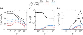
 ⟨IS⟩T
 ⟨IR⟩T
 ⟨IE⟩T
 a
 UW/δ
 b
 τηT−1
 c
 ⟨ε⟩T/u0T2
 Reθ=4000

 ⟨u′v′⟩
 a
 ⟨u′v′⟩=⟨uS′v′⟩+⟨uNS′v′⟩
 b
 ⟨u′v′⟩=⟨uS′vS′⟩+⟨uS′vNS′⟩+⟨uNS′vS′⟩+⟨uNS′vNS′⟩
 Reθ=4000

 z
 y
 x
 e1
 e2
 e3
 (e1)z
 (e2)y
 (e3)x
 a
 y+=15
 y/δ=0.0048
 b
 y+=31
 y/δ=0.01
 c
 y+=153
 y/δ=0.05
 d
 y+=1529
 y/δ=0.5
 Reθ=10000

 Reθ=10000
 IS¯
 (u1¯,u2¯,u3¯)
 a
 ζ2
 ζ3
 b
 ζ1
 ζ2
 y+=1529
 y/δ=0.5
 ⟨IS⟩T
 IS¯
 (IS¯)max

 y+=31
 y/δ=0.01

 y+=153
 y/δ=0.05

 ζ1
 ζ2
 Reθ=10000
 a
 y+=31
 y/δ=0.01
 b
 y+=153
 y/δ=0.05
 c
 y+=1529
 y/δ=0.5

 a
 b

 a,b
 y+=1529
 y/δ=0.5
 c,d
 y+=31
 y/δ=0.01
 Reθ=10000
 a,c
 u1¯
 ζ1
 b,d
 u2¯
 u3¯
 ζ2
 Δui
 δi

 a,c
 δ3
 b,d
 Δu3
 a
 b
 c
 δ3
 δν
 δν/τηT
 Δu3
 d
 a
 b
 δ3/ηT=4.7
 Δu3/uηT=6.9

 a
 δ3
 b
 Δu3
 u0T=(urmsT2+vrmsT2+wrmsT2)/3

 a,c
 δ1
 b,d
 Δu1
 a
 δ1/ηT
 b
 Δu1/uηT
 c
 δ1/δν
 d
 Δu1/(δν/τηT)
 a
 b
 δ1/ηT=8.9
 Δu1/uηT=2.2

 δ2
 Δu2
 a
 δ2/ηT
 b
 Δu2/uηT
 c
 δ2/δν
 d
 Δu2/(δν/τηT)
 a
 b
 δ2/ηT=17.2
 Δu2/uηT=2.1

 a
 δ1/ηT
 b
 Δu1/uηT
 y/δ

 a
 δ2/ηT
 b
 Δu2/uηT
 y/δ

 a
 δS/ηT
 b
 ΔuS/uηT
 c
 ReS
 d
 δS/δBV
 y+>50
 Reθ=4000

 a
 δS/ηT
 b
 ΔuS/uηT
 y/δ=0.2

 δS/δν
 ΔuS/(δν/τηT)
 ReS
 δS/δBV
 y+=15,20and30
 Reθ=4000and13000


