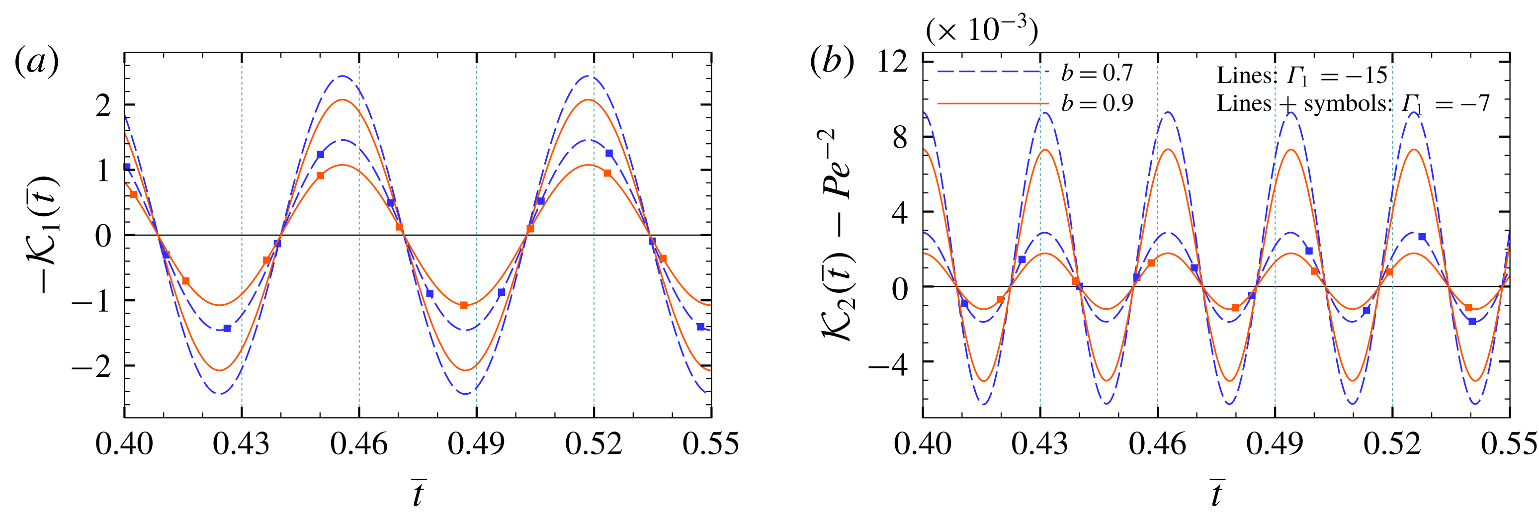
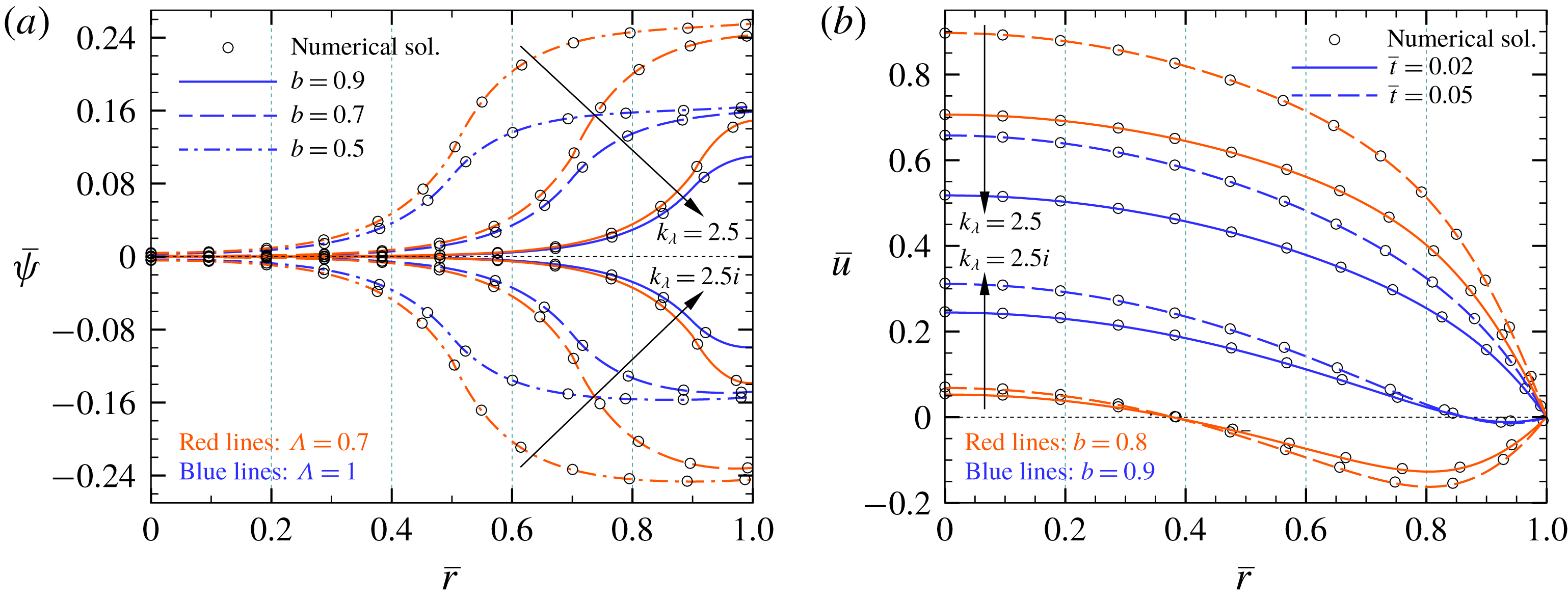
1 Introduction
During the past decades, the analysis of axial solute dispersion in micro/nanofluidic systems has received significant attention due to its practical importance in various applications, including micromixing (Huiqian, Nguyen & Huang Reference Huiqian, Nguyen and Huang2006; Leong et al. Reference Leong, Tsai, Chang, Lin and Fu2007), field flow fractionation and separation processes (Griffiths & Nilson Reference Griffiths and Nilson2006; Datta & Ghosal Reference Datta and Ghosal2008, Reference Datta and Ghosal2009), liquid chromatography (Van Theemsche et al. Reference Van Theemsche, Gzil, Dan, Deconinck, De Smet, Vervoort and Desmet2004; Xuan Reference Xuan2008) and capillary zone electrophoresis (Xuan & Li Reference Xuan and Li2004), among others. In this regard, depending on the type of the process, solute dispersion in the axial flow direction may have either positive or detrimental effects on the efficiency of the micro/nanoscale devices involved in species manipulation. For instance, the minimization of axial dispersion of merged chemical components is one of the design criteria for the optimization of analyte separation efficiency in micro/nanofluidic systems. In contrast, the dispersion phenomenon acts in favour of mixing operations, leading to a faster and more homogeneous dissolution of samples within the carrier fluid (Masliyah & Bhattacharjee Reference Masliyah and Bhattacharjee2006). With the aim of achieving precise control of solute species transport through lab-on-a-chip (LOC) devices, numerous theoretical and experimental studies have been conducted for the characterization and quantification of dispersion behaviour of samples under various operating conditions. A review of the literature on this subject reveals some practically realized mechanisms for the regulation of the dispersion mechanism in micro/nanofluidic systems, including the modulation of solute dispersion by transverse electric fields (Dutta Reference Dutta2015), controlling the dispersion characteristics of nanoparticles and solutes in microchannel flows by surface modification and functionalization (Faure et al. Reference Faure, Salazar-Alvarez, Ahniyaz, Villaluenga, Berriozabal, De Miguel and Bergström2013; Hoshyargar et al. Reference Hoshyargar, Khorami, Ashrafizadeh and Sadeghi2018) and the intensification of mixing processes using alternating current (AC) electrokinetic pumps (Lim, Lam & Yang Reference Lim, Lam and Yang2010; Lim & Lam Reference Lim and Lam2012; Alipanah & Ramiar Reference Alipanah and Ramiar2017).
The theoretical modelling of hydrodynamic dispersion in macroscale transport processes has been the subject of numerous studies over the past several decades and, subsequently, considerable efforts have been made towards the development of these methodologies for estimating the solute transport in micro/nanofluidic devices (Datta & Ghosal Reference Datta and Ghosal2009). Historically, the problem of passive solute dispersion in a pressure-driven Hagen–Poiseuille flow was first investigated by Taylor (Reference Taylor1953), who proposed an effective diffusion coefficient for this phenomenon. Shortly thereafter, Aris (Reference Aris1956) extended the problem by representing the method of moments for analysing the asymptotic behaviour of the second-order moment of concentration. It is noted that, as the Taylor’s classical dispersion model is based on the transverse mean concentration, an initial period of time is required for smoothing out the cross-sectional concentration variation by the radial diffusion of solute through the tube. The duration of this process in Taylor’s first estimation was scaled as
 $D_{m}t/R^{2}\approx O(0.1)$
, in which
 $t,D_{m}$
and
 $R$
are time, molecular diffusion and tube radius, respectively. As later shown by Ananthakrishnan, Gill & Barduhn (Reference Ananthakrishnan, Gill and Barduhn1965), the Taylor–Aris theory is merely capable of predicting the dispersion behaviour of solutes for late-time periods of the transport process (that is,
 $D_{m}t/R^{2}>0.8$
). Then, using the derivative expansion method, Gill & Sankarasubramanian (Reference Gill and Sankarasubramanian1970) presented a generalized dispersion model for estimating all-time evolution of the band broadening process. Also, some notable advancements in the analysis of solute dispersion at both transient and developed states of the transport process are summarized as follows: developing a two-time-scale perturbation method by Fife & Nicholes (Reference Fife and Nicholes1975), obtaining asymptotic estimations of small- and large-time development of solute dispersion with more precision by Stokes & Barton (Reference Stokes and Barton1990) and Phillips, Kaye & Robinson (Reference Phillips, Kaye and Robinson1995), and presenting the homogenization technique by Mei, Auriault & Ng (Reference Mei, Auriault and Ng1996).
Theoretically, the cross-sectional mean concentration profile of a solute band along the axial flow direction during the diffusion-like dispersion process at large times after the solute injection is described by a Gaussian distribution function (Wu & Chen Reference Wu and Chen2014). The change in the variance of the band during solute transport per unit axial migrated distance is referred to as the theoretical plate (or plate height) (Grimes et al. Reference Grimes, Lüdtke, Unger and Liapis2002; Zholkovskij, Masliyah & Yaroshchuk Reference Zholkovskij, Masliyah and Yaroshchuk2013). As the non-uniform distribution of velocity over the cross-section is responsible for the longitudinal hydrodynamic dispersion of the solute band during the displacement inside the straight confinements, any factor such as the type of the fluidic actuation mechanism affecting the flow hydrodynamics can play a role in modifying the theoretical plate. Among various techniques for fluid flow generation in LOC devices, electroosmotic pumps have gained considerable attention due to their several advantages, such as requiring no moving parts, easier fabrication and precise flow control (Moles Reference Moles2002; Stone, Stroock & Ajdari Reference Stone, Stroock and Ajdari2004). Electroosmosis stems from the interaction of the surface bound electrical double layer (EDL) (that is, a thin layer of accumulated counterions screening the charge of the ionizable surface) with an external or induced tangential electric field. In other words, the movement of counterions in the diffusive part of the EDL due to the presence of an either steady or time-varying axial electric field causes the motion of surrounding liquid by virtue of a viscous drag force and, consequently, results in the generation of electroosmotic flow through a narrow confinement. It has been demonstrated that the theoretical plate in electroosmotic flow with a plug-like velocity profile is much smaller than that in pressure-driven flow with a parabolic-shaped velocity distribution (Jorgenson & Lukacs Reference Jorgenson and Lukacs1981; Tsuda, Nomura & Nakagawa Reference Tsuda, Nomura and Nakagawa1982). Therefore, because of their ability to produce much smaller hydrodynamic dispersion, electrokinetic pumps are well-suited for improving the performance of on-chip chromatographic devices involved in the separation and detection of samples.
Several aspects of hydrodynamic dispersion in direct current (DC) electroosmosis have since been studied in the literature. One of the first experimental investigations of solute spreading through this type of flow was conducted by Pretorius, Hopkins & Schieke (Reference Pretorius, Hopkins and Schieke1974), who measured the plate heights in DC-electroosmosis-based liquid chromatography at different flow rates. In addition, one of the initial theoretical efforts towards the realization of axial dispersion through DC-electroosmotic flow was performed by Martin & Guiochon (Reference Martin and Guiochon1984), who presented an approximate analysis of electrokinetics-induced dispersion in open-tubular capillary liquid chromatography. Also, by taking into account the effect of an external pressure gradient in the capillary electrophoresis process, the analysis of solute dispersion in mixed electroosmotic–Poiseuille flows was carried out by Datta & Kotamarthi (Reference Datta and Kotamarthi1990). The researchers continued their efforts in this area to evaluate the role of various other aspects of electrokinetic phenomena in solute transport and mixing processes, including the influence of EDL overlap and high zeta potential on hydrodynamic dispersion (Griffiths & Nilson Reference Griffiths and Nilson2000), the effect of zeta potential disparity of microchannel walls on solute dispersion (Zholkovskij et al. Reference Zholkovskij, Masliyah and Yaroshchuk2013), the quantification of band spreading by DC-electroosmosis for different types of electrolyte solutions and channel geometries in the absence (Zholkovskij, Masliyah & Czarnecki Reference Zholkovskij, Masliyah and Czarnecki2003) and in the presence of an imposed axial pressure gradient (Zholkovskij & Masliyah Reference Zholkovskij and Masliyah2004), and the influence of electrokinetically induced secondary flows on hydrodynamic dispersion (Zhao & Bau Reference Zhao and Bau2007).
The majority of previous studies in the context of band broadening by steady electroosmotic flows have been conducted for bare-wall (or rigid) microchannels. Here, we focus on the case where the wall of the micro/nanoconfinement is coated by a layer of charged polyelectrolyte (PE) brushes. The grafted layer in such confinements (usually identified as soft confinements) comprises an assembly of charged polymer chains tethered to the solid wall of the channel. The use of such coating layers, also called polyelectrolyte layers (PELs), for creating soft-functionalized surfaces is considered as a highly promising technique to improve the performance of various micro/nanofluidic devices, like transistors and diodes (Lee et al. Reference Lee, Panzer, He, Lodge and Frisbie2007; Vilozny et al. Reference Vilozny, Wollenberg, Actis, Hwang, Singaram and Pourmand2013), mechanically responding nanovalves (Mertz et al. Reference Mertz, HEMMERLÉ, Mutterer, Ollivier, Voegel, Schaaf and Lavalle2007), nanofluidic energy converters (Patwary, Chen & Das Reference Patwary, Chen and Das2016), biosensors (Ali et al. Reference Ali, Yameen, Neumann, Ensinger, Knoll and Azzaroni2008), and current rectifiers (Ali et al. Reference Ali, Yameen, Cervera, Ramiìrez, Neumann, Ensinger, Knoll and Azzaroni2010). Also, the manipulation of several factors, such as the thickness and grafting density of polymer chains and the amount and sign of the polymer charges, allows precise control of ions and species transport in soft micro/nanoscale fluidic systems. Especially, as thoroughly discussed in our previous paper (Reshadi & Saidi Reference Reshadi and Saidi2018), regulating the permittivity difference between the PEL and bulk electrolyte solution provides an excellent means of enhancing the electro-chemo-mechanical energy conversion efficiency in soft nanofluidics. Generally, the PEL–electrolyte permittivity difference leads to partitioning of ions near the soft interfaces (Poddar et al. Reference Poddar, Maity, Bandopadhyay and Chakraborty2016; Reshadi & Saidi Reference Reshadi and Saidi2018). The emergence of such a phenomenon is also inferable from the electrostatic contribution of Born energy (Born Reference Born1920), and its influence on solute transport in polyelectrolyte (PE)-grafted micro/nanotubes has yet to be theoretically investigated.
Due to the large surface-area-to-volume ratios in micro/nanofluidic confinements, controlling the fluid-wall friction is a field of active research in LOC devices (Choi et al.
Reference Choi, Ulmanella, Kim, Ho and Kim2006; Teo & Khoo Reference Teo and Khoo2010). Several factors may contribute to the amount of interfacial drag force in such equipment: such as the presence of a layer of fluid with low density (Tretheway & Meinhart Reference Tretheway and Meinhart2004), roughness-induced hydrophobicity (Sbragaglia et al.
Reference Sbragaglia, Benzi, Biferale, Succi and Toschi2006), and the formation of gas nanobubbles on the channel surface (Tyrrell & Attard Reference Tyrrell and Attard2001; Steitz et al.
Reference Steitz, Gutberlet, Hauss, Klösgen, Krastev, Schemmel, Simonsen and Findenegg2003). Especially for the latter case, it has been demonstrated that, depending on the shape of the liquid–gas menisci, the gas nanobubbles trapped inside the roughness elements of the surface may either act as a lubricant promoting the flow rate, or may even increase the flow resistance of the channel as a result of liquid–gas protruding menisci (Steinberger et al.
Reference Steinberger, Cottin-Bizonne, Kleimann and Charlaix2007). Therefore, regulating the shape of the menisci of entrapped nanobubbles at the interface can be considered as a means of controlling the surface drag force in micro/nanofluidic systems. In a similar fashion, the charged polymer brushes at the interface would provide a mechanism of fine tuning the apparent surface friction over the walls of soft micro/nanochannels by either their amount of hydrodynamic resistance or the sign of their charges. The role of the latter factor can be explained as follows: the PE brushes grafted on a neutral polarizable surface may become either negatively or positively charged, depending on the acid-like (
 $\text{HA}\leftrightharpoons \text{A}^{-}+\text{H}^{+}$
) or base-like (
 $\text{B}+\text{H}_{2}\text{O}\leftrightharpoons \text{BH}^{+}+\text{O}\text{H}^{-}$
) ionization reaction of the PE chargeable sites within the electrolyte solution, respectively (Das et al.
Reference Das, Banik, Chen, Sinha and Mukherjee2015). Therefore, as the sign of the charges of PE brushes determines the direction of electrokinetic flow in the presence of a constant axial electric field, the pressure-driven flow component may be promoted or suppressed as a result of a favourable or adverse electrokinetic body force on the fluid, respectively. For the case of counteracting electrokinetic flow, some of the liquid inside the PEL may participate in the flow reversal. Therefore, similar to the situation engendered by the structured surfaces with entrapped nanobubbles (Hyväluoma & Harting Reference Hyväluoma and Harting2008), one may assume that there exists a negative effective slip length at the solid surface and, subsequently, a virtual no-slip plane is formed inside the channel (see figure 10
b). Particularly, the emergence of such stationary surface inside the soft micro/nanoconfinement is essential for the design of electrophoretic velocity measurement devices, such that, by placing a charged particle at such a stationary surface, the motion of particle is not affected by the flow of electrolyte solution (Shaw Reference Shaw1992; Masliyah & Bhattacharjee Reference Masliyah and Bhattacharjee2006).
Besides continuing efforts in using DC-electroosmotic pumps in LOC devices, the application of alternating current (AC) electrokinetic flow has also shown its capability in improving the performance of integrated micromixers and various circular chromatographic techniques (Debesset et al. Reference Debesset, Hayden, Dalton, Eijkel and Manz2004). This kind of fluidic transport mechanism offers numerous advantages, such as reducing the amount of Faradaic currents to prevent the formation of bubbles in the carrier fluid (Loucaides, Ramos & Georghiou Reference Loucaides, Ramos and Georghiou2007), generating complex flow patterns to meet the requirements of mixing processes (Sasaki, Kitamori & Kim Reference Sasaki, Kitamori and Kim2006), and propelling liquid in the closed-loop microchannels involved in cyclic separation techniques (Eijkel, Van Den Berg & Manz Reference Eijkel, Van Den Berg and Manz2004). Also, several studies have analysed the solute dispersion and mixing processes under various operating conditions of pulsatile electroosmotic flow in rigid confinements (Huang & Lai Reference Huang and Lai2006; Ramon, Agnon & Dosoretz Reference Ramon, Agnon and Dosoretz2011; Paul & Ng Reference Paul and Ng2012; Song, Ng & Law Reference Song, Ng and Law2014; Li & Jian Reference Li and Jian2017; Ramon Reference Ramon2017; Medina et al. Reference Medina, Toledo, MÉNDEZ and Bautista2018). However, no study has yet been reported in the literature examining the effect of the PEL on the dispersion characteristics of a solute band propelled by AC-electroosmotic flow. Previous theoretical investigations in the context of soft micro/nanofluidics have been mainly directed towards the analysis of the velocity distribution and ionic conductance in PE-grafted micro/nanoconfinements. To the best of the authors’ knowledge, the researchers have left several unanswered questions regarding (1) the effect of pulsatile electroosmotic flow on band broadening through soft micro/nanotubes, (2) ion partitioning effects on hydrodynamic dispersion, (3) the influence of wall absorption on the rate of solute dispersion in the presence of the PEL, (4) the behaviour of solute dispersion in the presence of an excess-constant DC electric field and constant pressure gradient added to pure oscillatory electroosmotic and pressure driving forces.
In order to fill the aforementioned gaps in the literature and provide further insight into how the charged PEL along with other electrokinetic phenomena affects the dispersion process, we theoretically and numerically analyse the broadening of an uncharged solute band by pulsatile mixed electroosmotic–pressure-driven flow in soft micro/nanotubes. Due to its practical importance in various biological transport processes (Mazumder & Mondal Reference Mazumder and Mondal2005), we also consider an irreversible first-order catalytic reaction at the wall of the tube in the present investigation. Taking into account the axial diffusion effects, the band broadening process is analysed by employing three modelling techniques, including the generalized dispersion model (Sankarasubramanian & Gill Reference Sankarasubramanian and Gill1973), Taylor–Aris dispersion theory (Taylor Reference Taylor1953; Aris Reference Aris1956) and full-scale spatiotemporal numerical simulation via a finite difference method (FDM). In the first analytical model, we aim to present a general solution of band spreading by considering the condition of an irreversible first-order catalytic reaction at the wall of the tube. This solution can be used to determine the all-time evolution of band broadening under different boundary conditions of constant surface charge density or constant surface potential, provided that the Debye–Hückel approximation remains valid. In the second analytical model, we derive a simplified asymptotic solution of hydrodynamic dispersion which is suggested for late-time evolution of the band broadening process. It is noteworthy that, in various situations such as drug dispersion in short human arteries (Lighthill Reference Lighthill1966), the length of the tube is so short that one needs to apply the first analytical model to study the early-phase transient period of dispersion. Also, for analysing the dispersion behaviour of the solute, we deal with a PE-grafted capillary having a circular cross-section geometry due to its resemblance to most in-vitro fluidic instruments involved in sample transport processes, such as protein and peptide transport through micro/nanopores (Chun & Stroeve Reference Chun and Stroeve2002; Khodabandehloo & Chen Reference Khodabandehloo and Chen2017), ion transport in switchable biomimetic pores (Yameen et al. Reference Yameen, Ali, Neumann, Ensinger, Knoll and Azzaroni2009), and DNA translocations through nanopores (Meller, Nivon & Branton Reference Meller, Nivon and Branton2001).
The rest of the paper is organized as follows: in the following section, the flow geometry is elucidated and the physical specification of the problem and assumptions are expressed. The mathematical formulation of the problem together with the analytical and numerical solutions are presented in § 3; the statistical parameters of solute concentration distribution are also defined in this section. After discussing the results in § 4, we end by summarizing our key scientific findings in § 5.
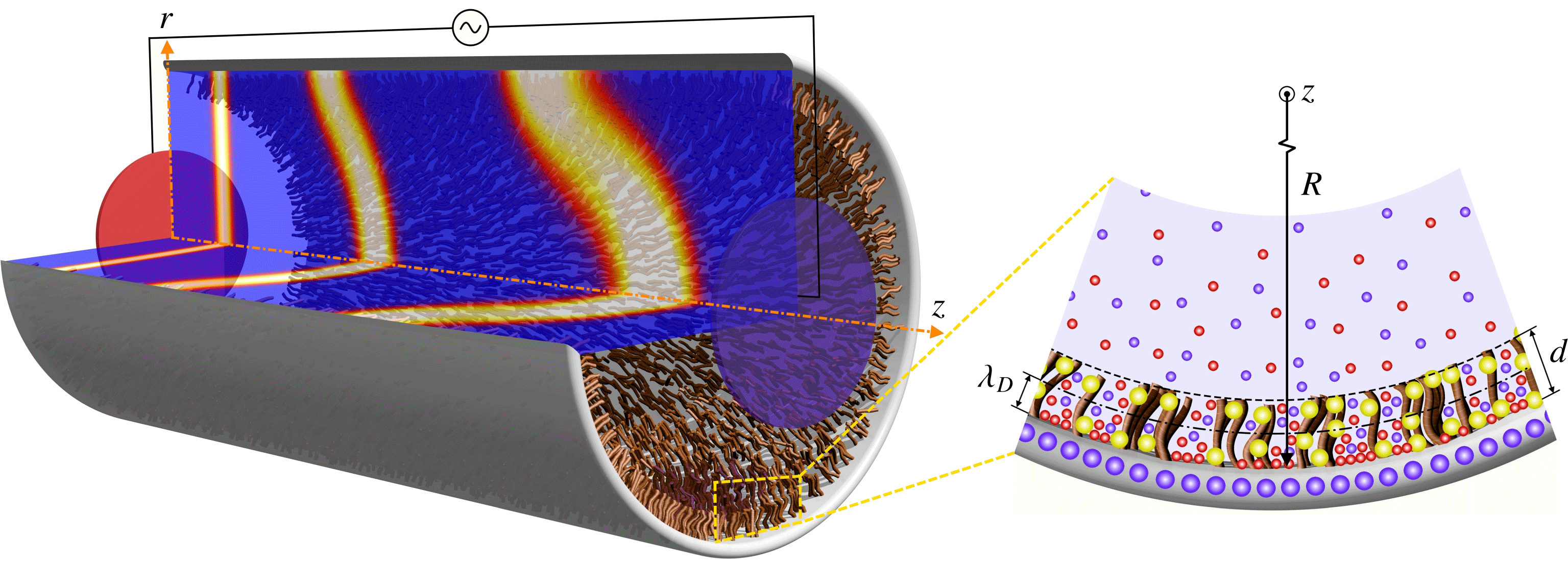
Schematic illustration of solute transport by pulsatile mixed electroosmotic–pressure-driven flow in a PE-grafted capillary of radius
 $R$
; the fixed charges of the PEL, the charges of the solid surface, counterions and coions in the electrolyte solution are illustrated by yellow, large blue, small red and small blue spheres, respectively, in the blown-up view.

2 Problem description and assumptions
Figure 1 schematically depicts a tube of radius
 $R$
on the wall of which a PEL of thickness
 $d$
is uniformly grafted. The cylindrical coordinate system
 $(r,z)$
, with the origin located at the centre of the tube, is employed for the analysis of hydrodynamic dispersion, where
 $r$
denotes the radial distance from the centre of the tube and
 $z$
is the axial coordinate. The distribution of ions inside the PEL and EDL in the vicinity of the charged wall of the tube is depicted in figure 1. As shown in this figure, the PEL contains uniformly distributed charges which stem from the ionization of PE chargeable sites and remain fixed within the PEL, while the electrolyte ions can exist both inside and outside the PEL. In order to generalize the present analysis, the electrical permittivity of the PEL is considered to be different from that of the bulk electrolyte solution. Also, under the influence of a DC/AC applied electric field produced by the external electrodes shown in figure 1, the net flux of counterions within the EDL of thickness
 $\unicode[STIX]{x1D706}_{D}$
is established towards the counter electrode. Consequently, the moving ions exert a viscous drag force on the electrolyte solution, resulting in the generation of axisymmetric DC/AC electroosmotic flow in the
 $z$
direction. Moreover, due to an additional pulsatile hydraulic actuation, the electroosmotic body force may be accompanied by a periodic pressure gradient operating at the same frequency as the applied electric field. To maintain the generality of the present model, in addition to the oscillatory components of electroosmotic and pressure driving forces, an excess-constant DC electric field and constant pressure gradient are considered as the steady parts of electrical and pressure driving forces, respectively. In the present study, we assume that the influence of flow-induced deformation of the PE brushes is negligible, and there is no significant change in the configuration of the end-tethered polymer chains due to the shear force exerted by the incompressible fluid flow (Chen & Das Reference Chen and Das2015a
,Reference Chen and Das
b
; Das et al.
Reference Das, Banik, Chen, Sinha and Mukherjee2015).
The dispersion process is started at time
 $t=0$
by instantaneous injection of a small amount of solute which is uniformly distributed over the cross-section of
 $z=0$
and is then propelled by pulsatile mixed electroosmotic–pressure-driven flow inside the soft capillary tube. Also, an irreversible first-order reaction catalysed by the tube wall gives rise to interfacial mass dissipation during the band broadening process. Moreover, the injected solute band is considered to be dilute enough so that the flow of carrier fluid is not affected by the presence of the sufficiently small soluble species. In the present study, after calculation of the electric potential distribution in the capillary, the dynamics of pulsatile mixed electroosmotic–pressure-driven flow is investigated; then, the dispersion characteristics of injected solute in the soft tube for two cases of steady and oscillatory flows will be analysed.
3 Analysis of electric potential, velocity and concentration fields
We carry out the analysis of pulsatile mixed electroosmotic–pressure-driven flow through the soft capillary shown in figure 1 by recalling the assumptions introduced in the previous section. The time-periodic flow velocity and solute concentration profile under consideration can be determined from the set of mass conservation, momentum and unsteady convection-diffusion equations. Accordingly, for a symmetric (
 $\unicode[STIX]{x1D56B}:\unicode[STIX]{x1D56B}$
) electrolyte solution, the equations of continuity, Navier–Stokes/Brinkman (NSB) and mass transport by pulsatile mixed electroosmotic–pressure-driven flow are, respectively, given as follows:
 $$\begin{eqnarray}\displaystyle & \displaystyle \unicode[STIX]{x1D735}\boldsymbol{\cdot }\boldsymbol{u}=0, & \displaystyle\end{eqnarray}$$
 $$\begin{eqnarray}\displaystyle & \displaystyle \unicode[STIX]{x1D70C}\frac{\unicode[STIX]{x2202}\boldsymbol{u}}{\unicode[STIX]{x2202}t}-\unicode[STIX]{x1D702}\unicode[STIX]{x1D6FB}^{2}\boldsymbol{u}=-\unicode[STIX]{x1D735}p(t)+\boldsymbol{F}_{\boldsymbol{ D}}+e\unicode[STIX]{x1D56B}(n_{+}-n_{-})\boldsymbol{E}(t), & \displaystyle\end{eqnarray}$$
 $$\begin{eqnarray}\displaystyle & \displaystyle \frac{\unicode[STIX]{x2202}c}{\unicode[STIX]{x2202}t}+\unicode[STIX]{x1D735}\boldsymbol{\cdot }(\boldsymbol{u}c)=D_{m}\unicode[STIX]{x1D735}\boldsymbol{\cdot }(\unicode[STIX]{x1D735}c), & \displaystyle\end{eqnarray}$$
where
 $\boldsymbol{u}=[0,0,u(r,t)]$
and
 $\boldsymbol{E}=[0,0,E_{z}(t)]$
are the velocity and the applied electric field vectors, respectively,
 $t$
is the time,
 $p(t)$
is the effective time-dependent pressure of the fluid, and
 $D_{m}$
and
 $c$
are the molecular diffusivity and concentration field of the solute, respectively. Also,
 $\unicode[STIX]{x1D56B}$
,
 $\unicode[STIX]{x1D70C}$
and
 $\unicode[STIX]{x1D702}$
are the ionic valence, the density and the dynamic viscosity of the electrolyte solution, respectively. The momentum equation (3.2) expresses the co-influence of inertia, viscosity, pressure, electrical driving force and hydrodynamic resistive force. The latter force is due to the presence of PE brushes in the wall-adherent region, which is zero outside the PEL. We model this force as
 $\boldsymbol{F}_{\boldsymbol{D}}=[0,0,-\mathbb{H}(r-B)\unicode[STIX]{x1D707}_{c}u]$
, where
 $\unicode[STIX]{x1D707}_{c}$
is the per unit volume friction coefficient associated with the resistance to the fluid movement induced by PEL,
 $B$
is the radial distance of the PEL–electrolyte interface from the centre of the capillary, and
 $\mathbb{H}(r-B)$
is the unit step function, whose value is
 $0$
or
 $1$
for the regions outside or inside the PEL, respectively. It is noted that the separation distance between the individual PE brushes is governed by the number density of polymer chains,
 $N_{p}$
. Also, the effective radius of the PE brushes is characterized by the equivalent Stokes radius of each polymer chain,
 $a$
. These two quantities affect the analysis through their relationship with the friction coefficient of the PEL, which is defined as
 $\unicode[STIX]{x1D707}_{c}=6\unicode[STIX]{x03C0}\unicode[STIX]{x1D702}aN_{p}$
(Wu & Keh Reference Wu and Keh2003). Finally,
 $n_{\pm }$
represents the number densities of electrolyte ions and can be obtained from the modified Poisson–Boltzmann equation which is introduced in the following subsection.
3.1 Modified Poisson–Boltzmann equation
In this subsection, we calculate the number densities of electrolyte ions by introducing the Poisson’s equation governing the electric potential distribution,
 $\unicode[STIX]{x1D713}(r)$
, inside the PE-grafted capillary as follows (Reshadi & Saidi Reference Reshadi and Saidi2018):
 $$\begin{eqnarray}\unicode[STIX]{x1D6FB}^{2}\unicode[STIX]{x1D713}=-\frac{e\unicode[STIX]{x1D56B}(n_{+}-n_{-})+\mathbb{H}(r-B)e\mathbb{Z}N}{\unicode[STIX]{x1D716}_{\unicode[STIX]{x1D556}}-\mathbb{H}(r-B)(\unicode[STIX]{x1D716}_{\unicode[STIX]{x1D556}}-\unicode[STIX]{x1D716}_{\unicode[STIX]{x1D561}})},\end{eqnarray}$$
where
 $e$
is the elementary charge,
 $\unicode[STIX]{x1D716}_{\unicode[STIX]{x1D556}}$
and
 $\unicode[STIX]{x1D716}_{\unicode[STIX]{x1D561}}$
are the permittivities of the bulk electrolyte and PEL domain, respectively, and
 $\mathbb{Z}$
and
 $N$
are the charge number (including its sign) and the number density of the fixed ions of the PEL, respectively. The last term in the numerator on the right-hand side of (3.4) is the charge density of the PEL,
 $\unicode[STIX]{x1D70C}_{f}$
. Since the PE chargeable sites are assumed to be uniformly distributed within the soft layer,
 $N$
is taken to be constant. Whereas from the electrostatic theory of aqueous electrolyte solutions near the charged surfaces,
 $n_{\pm }$
exhibit a spatial variation from the wall to the centre of the capillary. In this regard, by considering the equilibrium conditions of a symmetric electrolyte solution over the entire cross-section of capillary, the number densities of electrolyte ions are given as
 $n_{\pm }=n^{\infty }\exp [\mp e\unicode[STIX]{x1D56B}\unicode[STIX]{x1D713}/k_{B}T_{m}-\mathbb{H}(r-B)\unicode[STIX]{x0394}\unicode[STIX]{x1D707}_{\pm }]$
, where
 $n^{\infty }$
is the bulk ionic concentration,
 $k_{B}$
is the Boltzmann constant,
 $T_{m}$
is the average fluid temperature, and
 $\unicode[STIX]{x0394}\unicode[STIX]{x1D707}_{\pm }=e^{2}\unicode[STIX]{x1D56B}^{2}[\unicode[STIX]{x1D716}_{\unicode[STIX]{x1D561}}^{-1}-\unicode[STIX]{x1D716}_{\unicode[STIX]{x1D556}}^{-1}]/(8\unicode[STIX]{x03C0}k_{B}T_{m}\unicode[STIX]{x1D563}_{\pm })$
denotes the change in the free energy of electrolyte ions due to the Born dielectric effect, in which
 $\unicode[STIX]{x1D563}_{\pm }$
are the hydration radii of electrolyte ions. This equation for
 $n_{\pm }$
results from free energy minimization for a point charge model of ions (Reshadi & Saidi Reference Reshadi and Saidi2018).
Let us consider a symmetric electrolyte medium such as an aqueous solution of KCl in which cations and anions have approximately the same hydration radius – that is,
 $\unicode[STIX]{x1D563}_{+}\approx \unicode[STIX]{x1D563}_{-}$
(Israelachvili Reference Israelachvili2011). For such a system, the value of
 $\unicode[STIX]{x0394}\unicode[STIX]{x1D707}_{\pm }$
is identical for both cations and anions. By considering this point and substituting the aforementioned expression for
 $n_{\pm }$
into (3.4), we arrive at the following equation governing the electric potential distribution inside the PE-grafted capillary:
 $$\begin{eqnarray}\unicode[STIX]{x1D6FB}^{2}\unicode[STIX]{x1D713}=\frac{2e\unicode[STIX]{x1D56B}n^{\infty }\exp [-\mathbb{H}(r-B)\unicode[STIX]{x0394}\unicode[STIX]{x1D707}_{\pm }]\sinh (e\unicode[STIX]{x1D56B}\unicode[STIX]{x1D713}/k_{B}T_{m})-\mathbb{H}(r-B)e\mathbb{Z}N}{\unicode[STIX]{x1D716}_{\unicode[STIX]{x1D556}}+\mathbb{H}(r-B)(\unicode[STIX]{x1D716}_{\unicode[STIX]{x1D561}}-\unicode[STIX]{x1D716}_{\unicode[STIX]{x1D556}})}.\end{eqnarray}$$
It is noteworthy that, as the PEL-charge density is assumed to be constant, this layer is identified as the fixed charge layer (FCL). For a symmetric electrolyte solution in a micro/nanotube with low surface potential (
 $\unicode[STIX]{x1D713}_{0}<26$
mV), we may express (3.5) in the present cylindrical coordinates and invoke the Debye–Hückel approximation (Li Reference Li2004) to obtain the linearized dimensionless form of the Poisson–Boltzmann equation as follows:
 $$\begin{eqnarray}\frac{1}{\bar{r}}\frac{\text{d}}{\text{d}\bar{r}}\left(\bar{r}\frac{\text{d}\bar{\unicode[STIX]{x1D713}}}{\text{d}\bar{r}}\right)=\frac{K^{2}\{\bar{\unicode[STIX]{x1D713}}\exp [\mathbb{H}(\bar{r}-b)\unicode[STIX]{x1D714}(1-\unicode[STIX]{x1D6EC}^{-1})]-\mathbb{H}(\bar{r}-b)k_{\unicode[STIX]{x1D706}}^{-2}\}}{1+\mathbb{H}(\bar{r}-b)(\unicode[STIX]{x1D6EC}-1)},\end{eqnarray}$$
where the following set of dimensionless quantities are defined:
 $\bar{r}=r/R$
,
 $b=B/R$
,
 $\bar{\unicode[STIX]{x1D713}}=e\unicode[STIX]{x1D56B}\unicode[STIX]{x1D713}/k_{B}T_{m}$
,
 $\unicode[STIX]{x1D6EC}=\unicode[STIX]{x1D716}_{p}/\unicode[STIX]{x1D716}_{e}$
, and
 $K=R/\unicode[STIX]{x1D706}_{D}$
is the dimensionless Debye–Hückel parameter, in which
 $\unicode[STIX]{x1D706}_{D}=(2n^{\infty }e^{2}\unicode[STIX]{x1D56B}^{2}/\unicode[STIX]{x1D716}_{\unicode[STIX]{x1D556}}k_{B}T_{m})^{-1/2}$
is the Debye length. Also,
 $\unicode[STIX]{x1D714}=\unicode[STIX]{x1D706}_{D}^{-2}/16n^{\infty }\unicode[STIX]{x03C0}\unicode[STIX]{x1D563}_{\pm }$
and
 $k_{\unicode[STIX]{x1D706}}=\unicode[STIX]{x1D706}_{PEL}/\unicode[STIX]{x1D706}_{D}$
is the ratio of the equivalent EDL thickness inside the PEL (defined as
 $\unicode[STIX]{x1D706}_{PEL}=(Ne^{2}\unicode[STIX]{x1D56B}\mathbb{Z}/\unicode[STIX]{x1D716}_{\unicode[STIX]{x1D556}}k_{B}T_{m})^{-1/2}$
) to the Debye length. The appropriate conditions for solving (3.6) are specified as: (a) the finiteness of
 $\bar{\unicode[STIX]{x1D713}}$
at the centre of the capillary, (b) the axial symmetry condition for
 $\bar{\unicode[STIX]{x1D713}}$
, (c) the continuity requirement of electric potential, (d) the continuity of the electric displacement, and (e) equality of
 $\bar{\unicode[STIX]{x1D713}}$
and the dimensionless surface potential (
 $\bar{\unicode[STIX]{x1D713}}_{0}=e\unicode[STIX]{x1D56B}\unicode[STIX]{x1D713}_{0}/k_{B}T_{m}$
) at the wall of the capillary, which can be expressed, respectively, in the following dimensionless forms:
 $$\begin{eqnarray}\displaystyle \left.\begin{array}{@{}c@{}}\displaystyle \bar{\unicode[STIX]{x1D713}}_{\unicode[STIX]{x1D556}}|_{\bar{r}=0}=\text{finite},\quad \left.\frac{\text{d}\bar{\unicode[STIX]{x1D713}}_{\unicode[STIX]{x1D556}}}{\text{d}\bar{r}}\right|_{\bar{r}=0}=0,\quad \bar{\unicode[STIX]{x1D713}}_{\unicode[STIX]{x1D556}}|_{\bar{r}=b^{-}}=\bar{\unicode[STIX]{x1D713}}_{\unicode[STIX]{x1D561}}|_{\bar{r}=b^{+}},\\ \displaystyle \left.\frac{\text{d}\bar{\unicode[STIX]{x1D713}}_{\unicode[STIX]{x1D556}}}{\text{d}\bar{r}}\right|_{\bar{r}=b^{-}}=\unicode[STIX]{x1D6EC}\left.\frac{\text{d}\bar{\unicode[STIX]{x1D713}}_{\unicode[STIX]{x1D561}}}{\text{d}\bar{r}}\right|_{\bar{r}=b^{+}},\quad \bar{\unicode[STIX]{x1D713}}_{\unicode[STIX]{x1D561}}|_{\bar{r}=1}=\bar{\unicode[STIX]{x1D713}}_{0},\end{array}\right\} & & \displaystyle\end{eqnarray}$$
where the subscripts
 $\unicode[STIX]{x1D556}$
and
 $\unicode[STIX]{x1D561}$
refer to the electrolyte medium and the PEL domain, respectively. It is noted that the electric potential at the surface of the capillary is considered to be approximately equal to that in the shear plane (that is, the zeta potential) (Hunter Reference Hunter1988). Therefore, by employing the above conditions, the analytical solutions of (3.6) outside and inside the PEL domain can be obtained as follows:
 $$\begin{eqnarray}\displaystyle & \displaystyle \bar{\unicode[STIX]{x1D713}}_{\unicode[STIX]{x1D556}}=C_{1}\text{I}_{0}(K\bar{r}), & \displaystyle\end{eqnarray}$$
 $$\begin{eqnarray}\displaystyle & \displaystyle \bar{\unicode[STIX]{x1D713}}_{\unicode[STIX]{x1D561}}=C_{2}\text{I}_{0}(J\bar{r})+C_{3}\text{K}_{0}(J\bar{r})+C_{4}, & \displaystyle\end{eqnarray}$$
 $J=K\exp [\unicode[STIX]{x1D714}(1-\unicode[STIX]{x1D6EC}^{-1})/2]/\sqrt{\unicode[STIX]{x1D6EC}}$
and
 $\text{I}_{0}$
and
 $\text{K}_{0}$
are the zeroth-order modified Bessel functions of the first and second kinds, respectively. Also, the constant coefficients
 $C_{1-4}$
are given in appendix B. If, instead of the surface potential, the value of the surface charge density (
 $\unicode[STIX]{x1D70E}$
) is given at the inner wall of the capillary, the Gauss law may be used to obtain the electrostatic boundary condition at the PEL–wall interface, such that the boundary condition (3.7e
) must be replaced by
 $\text{d}\bar{\unicode[STIX]{x1D713}}_{\unicode[STIX]{x1D561}}/\text{d}\bar{r}=\bar{\unicode[STIX]{x1D70E}}$
at
 $\bar{r}=1$
, in which
 $\bar{\unicode[STIX]{x1D70E}}=\unicode[STIX]{x1D70E}e\unicode[STIX]{x1D56B}R/(\unicode[STIX]{x1D716}_{\unicode[STIX]{x1D561}}k_{B}T_{m})$
is the dimensionless surface charge density. In this regard, after some mathematical manipulations that are not presented here for the sake of brevity, the following relationship between the electric potential and surface charge density at the wall of the capillary can be obtained:
 $$\begin{eqnarray}\displaystyle \bar{\unicode[STIX]{x1D713}}_{0} & = & \displaystyle -\left\{K\text{I}_{1}\right.\!(bK)[C_{4}-(\bar{\unicode[STIX]{x1D70E}}\text{I}_{0}(J)+C_{4}J\text{I}_{1}(J))\text{K}_{0}(bJ)+\text{I}_{0}(bJ)(\bar{\unicode[STIX]{x1D70E}}\text{K}_{0}(J)-C_{4}J\text{K}_{1}(J))]\nonumber\\ \displaystyle & & \displaystyle \left.+\,J\unicode[STIX]{x1D6EC}\text{I}_{0}(bK)[\text{I}_{1}(bJ)(-\bar{\unicode[STIX]{x1D70E}}\text{K}_{0}(J)+C_{4}J\text{K}_{1}(J))-(\bar{\unicode[STIX]{x1D70E}}\text{I}_{0}(J)+C_{4}J\text{I}_{1}(J))\text{K}_{1}(bJ)]\right\}\nonumber\\ \displaystyle & & \displaystyle \times \,\left\{-J^{2}\unicode[STIX]{x1D6EC}\text{I}_{0}(bK)\text{I}_{1}(bJ)\text{K}_{1}(J)+KJ\text{I}_{1}(bK)[\text{I}_{1}(J)\text{K}_{0}(bJ)+\text{I}_{0}(bJ)\text{K}_{1}(J)]\right.\nonumber\\ \displaystyle & & \displaystyle \left.+\,J^{2}\unicode[STIX]{x1D6EC}\text{I}_{0}(bK)\text{I}_{1}(J)\text{K}_{1}(bJ)\right\}^{-1},\end{eqnarray}$$
where
 $\text{I}_{1}$
and
 $\text{K}_{1}$
are the first-order modified Bessel functions of the first and second kinds, respectively. If the value of the dimensionless surface charge density is given, the value of
 $\bar{\unicode[STIX]{x1D713}}_{0}$
can be evaluated from (3.9) and, consequently, the electric potential distribution may be obtained through the use of (3.8a
) and (3.8b
).
3.2 Momentum balance in the axial direction
Having obtained the electric potential distribution inside the soft capillary, the electrokinetic body force in the NSB equation – that is, the last term on the right-hand side of (3.2) – can be evaluated and, therefore, we may now proceed to calculate the time-dependent velocity profile from the NSB equation. By performing some mathematical manipulations, the dimensionless equation governing the axisymmetric mixed electroosmotic–Poiseuille flow velocity in the present cylindrical coordinates can be expressed as follows:
 $$\begin{eqnarray}\frac{1}{Sc}\frac{\unicode[STIX]{x2202}\bar{u}}{\unicode[STIX]{x2202}\bar{t}}-\frac{1}{\bar{r}}\frac{\unicode[STIX]{x2202}}{\unicode[STIX]{x2202}\bar{r}}\left(\bar{r}\frac{\unicode[STIX]{x2202}\bar{u}}{\unicode[STIX]{x2202}\bar{r}}\right)=-\bar{p}_{,z}(\bar{t})-\mathbb{H}(\bar{r}-b)\unicode[STIX]{x1D6FC}^{2}\bar{u}+K^{2}\exp [\mathbb{H}(\bar{r}-b)\unicode[STIX]{x1D714}(1-\unicode[STIX]{x1D6EC}^{-1})]\bar{\unicode[STIX]{x1D713}}\bar{E}_{z}(\bar{t}).\end{eqnarray}$$
In the above equation, the dimensionless quantities are defined as follows:
 $\bar{E}_{z}(\bar{t})=E_{z}(t)/E_{c}$
and
 $\bar{p}_{,z}(\bar{t})=p_{,z}(t)R^{2}/\unicode[STIX]{x1D702}u_{HS}$
are the dimensionless time-periodic electric field and the dimensionless pulsatile axial pressure gradient, respectively, which are assumed to be applied at the same angular frequency (
 $\unicode[STIX]{x1D6FA}$
). Also,
 $\bar{u}=u/u_{HS}$
is the dimensionless axial velocity and
 $\unicode[STIX]{x1D6FC}=R\sqrt{\unicode[STIX]{x1D707}_{c}/\unicode[STIX]{x1D702}}$
is the ratio of channel radius to the characteristic penetration length of the flow inside the PEL (Duval et al.
Reference Duval, Wilkinson, Van Leeuwen and Buffle2005). In these quantities,
 $u_{HS}=-\unicode[STIX]{x1D716}_{\unicode[STIX]{x1D556}}k_{B}T_{m}E_{c}/e\unicode[STIX]{x1D56B}\unicode[STIX]{x1D702}$
is the characteristic velocity of electroosmotic flow (Probstein Reference Probstein2005) and
 $E_{c}$
is the characteristic electric field. In addition,
 $Sc=\unicode[STIX]{x1D710}/D_{m}$
is the Schmidt number – defined as the ratio of the kinematic viscosity (
 $\unicode[STIX]{x1D710}$
) to the molecular diffusion coefficient (
 $D_{m}$
) – and
 $\bar{t}=D_{m}t/R^{2}$
is the dimensionless time. The required conditions for solving (3.10) are defined as: (a) the finiteness of
 $\bar{u}$
at the centre of the capillary, (b) the axial symmetry condition for
 $\bar{u}$
, (c) the continuity requirement of velocity, (d) the continuity of shear stress, and (e) the no-slip condition at the wall of the capillary, which can be expressed, respectively, in the following dimensionless forms:
 $$\begin{eqnarray}\displaystyle \left.\begin{array}{@{}c@{}}\displaystyle \left.\bar{u}_{\unicode[STIX]{x1D556}}\right|_{\bar{r}=0}=\text{finite},\quad \left.\frac{\text{d}\bar{u}_{\unicode[STIX]{x1D556}}}{\text{d}\bar{r}}\right|_{\bar{r}=0}=0,\quad \left.\bar{u}_{\unicode[STIX]{x1D556}}\right|_{\bar{r}=b^{-}}=\left.\bar{u}_{\unicode[STIX]{x1D561}}\right|_{\bar{r}=b^{+}},\\ \displaystyle \left.\frac{\text{d}\bar{u}_{\unicode[STIX]{x1D556}}}{\text{d}\bar{r}}\right|_{\bar{r}=b^{-}}=\left.\frac{\text{d}\bar{u}_{\unicode[STIX]{x1D561}}}{\text{d}\bar{r}}\right|_{\bar{r}=b^{+}},\quad \left.\bar{u}_{\unicode[STIX]{x1D561}}\right|_{\bar{r}=1}=0.\end{array}\right\} & & \displaystyle\end{eqnarray}$$
As discussed before, the applied pressure gradient, axial electric field and the resulting flow velocity comprise the steady and harmonically fluctuating components oscillating at the same angular frequency (
 $\unicode[STIX]{x1D6FA}$
). Therefore, we can express these three quantities in the dimensionless forms as follows (Huang & Lai Reference Huang and Lai2006; Li & Jian Reference Li and Jian2017):
 $$\begin{eqnarray}\langle \bar{E}_{z}(\bar{t}),\bar{p}_{,z}(\bar{t}),\bar{u}(\bar{r},\bar{t})\rangle =\langle \bar{E}_{z0},\unicode[STIX]{x1D6E4}_{0},\bar{u}_{0}(\bar{r})\rangle +\text{Im}\{\langle \bar{E}_{z1},\unicode[STIX]{x1D6E4}_{1},\bar{u}_{1}(\bar{r})\rangle \exp (\text{i}\mathit{Re}Sc\bar{t})\},\end{eqnarray}$$
where
 $[\unicode[STIX]{x1D6E4}_{0},\unicode[STIX]{x1D6E4}_{1}]=[p_{0,z},p_{1,z}]R^{2}/(\unicode[STIX]{x1D702}u_{HS})$
,
 $[\bar{u}_{0},\bar{u}_{1}]=[u_{0},u_{1}]/u_{HS}$
and
 $[\bar{E}_{z0},\bar{E}_{z1}]=[E_{z0},E_{z1}]/E_{c}$
, in which subscripts 0 and 1 refer to the steady part and the amplitude of the oscillatory component of each quantity, respectively. Also,
 $\text{i}=\sqrt{-1}$
is the imaginary unit number,
 $\text{Im}\{\,\}$
indicates the imaginary part of a complex number, and
 $\mathit{Re}=\unicode[STIX]{x1D70C}\unicode[STIX]{x1D6FA}R^{2}/\unicode[STIX]{x1D702}$
is the oscillating Reynolds number, which is also proportional to the square of the Womersley number for pulsatile blood flows through arteries (Mazumder & Mondal Reference Mazumder and Mondal2005). As (3.10) is linear in pressure, electric field and velocity, this equation can deal with steady and oscillatory parts of the flow separately (Chakraborty & Ray Reference Chakraborty and Ray2008). Therefore, substituting equation (3.12) into (3.10) and equating the coefficients of
 $\exp (\text{i}ReSc\bar{t})$
in both sides of the resulting equation, one may obtain:
 $$\begin{eqnarray}\displaystyle & \displaystyle \frac{1}{\bar{r}}\frac{\text{d}}{\text{d}\bar{r}}\left(\bar{r}\frac{\text{d}\bar{u}_{0}}{\text{d}\bar{r}}\right)=\unicode[STIX]{x1D6E4}_{0}+\mathbb{H}(\bar{r}-b)\unicode[STIX]{x1D6FC}^{2}\bar{u}_{0}-K^{2}\exp [\mathbb{H}(\bar{r}-b)\unicode[STIX]{x1D714}(1-\unicode[STIX]{x1D6EC}^{-1})]\bar{\unicode[STIX]{x1D713}}\bar{E}_{z0}, & \displaystyle\end{eqnarray}$$
 $$\begin{eqnarray}\displaystyle & \displaystyle \frac{1}{\bar{r}}\frac{\unicode[STIX]{x2202}}{\unicode[STIX]{x2202}\bar{r}}\left(\bar{r}\frac{\unicode[STIX]{x2202}\bar{u}_{1}}{\unicode[STIX]{x2202}\bar{r}}\right)=\unicode[STIX]{x1D6E4}_{1}+\{\mathbb{H}(\bar{r}-b)\unicode[STIX]{x1D6FC}^{2}+\text{i}Re\}\bar{u}_{1}-K^{2}\exp [\mathbb{H}(\bar{r}-b)\unicode[STIX]{x1D714}(1-\unicode[STIX]{x1D6EC}^{-1})]\bar{\unicode[STIX]{x1D713}}\bar{E}_{z1}. & \displaystyle \nonumber\\ \displaystyle & & \displaystyle\end{eqnarray}$$
It is noteworthy that the conditions of (3.11 a–e
) hold for both
 $\bar{u}_{0}$
and
 $\bar{u}_{1}$
. Therefore, under such imposed conditions, the solutions of (3.13) and (3.14) outside and inside the PEL domain can be determined as follows:
 $$\begin{eqnarray}\bar{u}_{\unicode[STIX]{x1D556}0}(\bar{r})=\{M_{1}-C_{1}\text{I}_{0}(K\bar{r})\}\bar{E}_{z0}+\{\bar{r}^{2}/4+M_{2}\}\unicode[STIX]{x1D6E4}_{0},\end{eqnarray}$$
 $$\begin{eqnarray}\displaystyle \bar{u}_{\unicode[STIX]{x1D561}0}(\bar{r}) & = & \displaystyle \left\{M_{3}\text{K}_{0}(\unicode[STIX]{x1D6FC}\bar{r})+M_{4}\text{I}_{0}(\unicode[STIX]{x1D6FC}\bar{r})+J^{2}\unicode[STIX]{x1D6EC}[C_{2}\text{I}_{0}(J\bar{r})+C_{3}\text{K}_{0}(J\bar{r})]/(\unicode[STIX]{x1D6FC}^{2}-J^{2})\right.\nonumber\\ \displaystyle & & \displaystyle \left.+\,C_{4}J^{2}\unicode[STIX]{x1D6EC}\unicode[STIX]{x1D6FC}^{-2}\right\}\bar{E}_{z0}+\{M_{5}\text{K}_{0}(\unicode[STIX]{x1D6FC}\bar{r})+M_{6}\text{I}_{0}(\unicode[STIX]{x1D6FC}\bar{r})-\unicode[STIX]{x1D6FC}^{-2}\}\unicode[STIX]{x1D6E4}_{0},\end{eqnarray}$$
 $$\begin{eqnarray}\bar{u}_{\unicode[STIX]{x1D556}1}(\bar{r})=\{N_{1}\text{I}_{0}(k_{1}\bar{r})+K^{2}C_{1}k_{1}\text{I}_{0}(K\bar{r})/[k_{1}(k_{1}^{2}-K^{2})]\}\bar{E}_{z1}+\{N_{2}\text{I}_{0}(k_{1}\bar{r})-k_{1}^{-2}\}\unicode[STIX]{x1D6E4}_{1},\end{eqnarray}$$
 $$\begin{eqnarray}\displaystyle \bar{u}_{\unicode[STIX]{x1D561}1}(\bar{r}) & = & \displaystyle \left\{N_{3}\text{I}_{0}(k_{2}\bar{r})+N_{4}\text{K}_{0}(k_{2}\bar{r})+J^{2}\unicode[STIX]{x1D6EC}[C_{2}\text{I}_{0}(J\bar{r})+C_{3}\text{K}_{0}(J\bar{r})]/(k_{2}^{2}-J^{2})\right.\nonumber\\ \displaystyle & & \displaystyle \left.+\,C_{4}J^{2}\unicode[STIX]{x1D6EC}k_{2}^{-2}\right\}\bar{E}_{z1}+\{N_{5}\text{I}_{0}(k_{2}\bar{r})+N_{6}\text{K}_{0}(k_{2}\bar{r})-k_{2}^{-2}\}\unicode[STIX]{x1D6E4}_{1},\end{eqnarray}$$
where the subscripts
 $\unicode[STIX]{x1D556}$
and
 $\unicode[STIX]{x1D561}$
refer to the solutions of velocity components in the electrolyte medium and the PEL domain, respectively. Also,
 $k_{1}^{2}=\text{i}Re$
,
 $k_{2}^{2}=\unicode[STIX]{x1D6FC}^{2}+\text{i}Re$
, and the coefficients
 $M_{1-6}$
and
 $N_{1-6}$
are given in appendix B.
3.3 Analysis of solute dispersion
The unsteady band broadening due to the flow of solvent and molecular diffusion of solute is governed by (3.3). Under the present cylindrical coordinates, this equation together with the associated conditions can be expressed in the dimensionless forms as follows:
 $$\begin{eqnarray}\frac{\unicode[STIX]{x2202}\bar{c}}{\unicode[STIX]{x2202}\bar{t}}+\bar{u}\frac{\unicode[STIX]{x2202}\bar{c}}{\unicode[STIX]{x2202}\bar{z}}=\frac{1}{\bar{r}}\frac{\unicode[STIX]{x2202}}{\unicode[STIX]{x2202}\bar{r}}\left(\bar{r}\frac{\unicode[STIX]{x2202}\bar{c}}{\unicode[STIX]{x2202}\bar{r}}\right)+\frac{1}{Pe^{2}}\frac{\unicode[STIX]{x2202}^{2}\bar{c}}{\unicode[STIX]{x2202}\bar{z}^{2}};\quad 0\leqslant \bar{r}\leqslant 1,~\left|\bar{z}\right|<\infty ,\end{eqnarray}$$
 $$\begin{eqnarray}\displaystyle \left.\begin{array}{@{}c@{}}\displaystyle \left.\frac{\unicode[STIX]{x2202}\bar{c}}{\unicode[STIX]{x2202}\bar{r}}\right|_{\bar{r}=0}=0,\quad \left.\frac{\unicode[STIX]{x2202}\bar{c}}{\unicode[STIX]{x2202}\bar{r}}\right|_{\bar{r}=1}=-\unicode[STIX]{x1D6FD}\left.\bar{c}\right|_{\bar{r}=1},\\ \displaystyle \bar{c}|_{\bar{z}\rightarrow \pm \infty }=\left.\frac{\unicode[STIX]{x2202}\bar{c}}{\unicode[STIX]{x2202}\bar{z}}\right|_{\bar{z}\rightarrow \pm \infty }=0,\quad \bar{c}|_{\bar{t}=0}=\bar{\unicode[STIX]{x1D6F9}}(\bar{z})\bar{Y}(\bar{r}),\end{array}\right\} & & \displaystyle\end{eqnarray}$$
where the above dimensionless quantities are defined as follows:
 $\bar{c}=c/C_{0}$
is the dimensionless concentration (that is, scaled by
 $C_{0}=M_{0}/\unicode[STIX]{x03C0}R^{3}$
, in which
 $M_{0}$
is the total mass of the injected solute). Also,
 $Pe=|u_{HS}|R/D_{m}$
is the Péclet number and
 $\bar{z}=zD_{m}/(u_{HS}R^{2})$
is the dimensionless axial coordinate. In the above equation, the condition (a) denotes the axisymmetric distribution of the solute band inside the capillary and the condition (b) denotes the irreversible first-order catalytic reaction at the wall of the capillary, whose reaction rate constant is
 $k$
. The coefficient
 $k$
in (3.20b
) is scaled as
 $\unicode[STIX]{x1D6FD}=kR/D_{m}$
, which characterizes the rate of irreversible absorption of solute into the wall of the capillary (Ng & Rudraiah Reference Ng and Rudraiah2008). Also, the condition of zero concentration at infinity in (3.20c
) stands for the finiteness of the injected solute cloud inside the capillary, and the condition of zero flux of concentration at infinity corresponds to the mathematical requirement for obtaining the analytical solution of the present problem. The mathematical formulation for the initial condition of the released solute inside the capillary is described by (3.20d
), in which
 $\bar{\unicode[STIX]{x1D6F9}}(\bar{z})=\unicode[STIX]{x1D6FF}^{\prime }(\bar{z})/Pe$
and
 $\bar{Y}(\bar{r})=1$
are the dimensionless axial and radial distribution functions corresponding to the primary pulse of injected solute occupying the entire cross-section of the capillary. Here,
 $\unicode[STIX]{x1D6FF}^{\prime }(\bar{z})$
is the Dirac delta function. In order to solve the above transport equation, we consider three approaches, namely, (1) the generalized dispersion method, (2) the Taylor–Aris dispersion theory, and (3) custom-built full-scale numerical simulation using the FDM. As will be shown in the next subsections, although the first approach predicts the structure of dispersion at small and large time periods of solute transport, it introduces a great deal of complexity into the solution procedure. Therefore, for the limiting case of a non-reacting wall of the capillary, the use of the second analytical approach with a simpler formulation is suggested for investigating the late-time evolution of the band broadening process.
3.3.1 Generalized dispersion model
In this subsection, the generalized dispersion model is employed to determine the all-time evolution of solute dispersion by pulsatile mixed electroosmotic–Poiseuille flow in the soft capillary. Following this method, the dimensionless solute concentration,
 $\bar{c}(\bar{r},\bar{z},\bar{t})$
, is expanded in terms of partial derivatives of the transverse mean concentration,
 $\bar{c}_{m}(\bar{z},\bar{t})$
, with respect to the axial coordinate to arrive at the following infinite series:
 $$\begin{eqnarray}\bar{c}(\bar{r},\bar{z},\bar{t})=\mathop{\sum }_{i=0}^{\infty }f_{i}(\bar{r},\bar{t})\frac{\unicode[STIX]{x2202}^{i}\bar{c}_{m}(\bar{z},\bar{t})}{\unicode[STIX]{x2202}\bar{z}^{i}},\end{eqnarray}$$
where
 $\bar{c}_{m}\left(\bar{z},\bar{t}\right)=2\int _{0}^{1}\bar{c}\bar{r}\,\text{d}\bar{r}$
, and
 $f_{i}(\bar{r},\bar{t})$
are the series coefficients. In order to evaluate the cross-sectional average of (3.19), we multiply both sides of this equation by
 $2\bar{r}$
, and then we integrate the resulting equation with respect to
 $\bar{r}$
from
 $0$
to
 $1$
to obtain the following relation:
 $$\begin{eqnarray}\frac{\unicode[STIX]{x2202}\bar{c}_{m}}{\unicode[STIX]{x2202}\bar{t}}=\frac{1}{Pe^{2}}\frac{\unicode[STIX]{x2202}^{2}\bar{c}_{m}}{\unicode[STIX]{x2202}\bar{z}^{2}}+2\left.\frac{\unicode[STIX]{x2202}\bar{c}}{\unicode[STIX]{x2202}\bar{r}}\right|_{\bar{r}=1}-2\frac{\unicode[STIX]{x2202}}{\unicode[STIX]{x2202}\bar{z}}\int _{0}^{1}\bar{u}\bar{c}\bar{r}\,\text{d}\bar{r}.\end{eqnarray}$$
After substituting the corresponding expression for the concentration from (3.21) into (3.22), and by appropriate rearranging, the following generalized dispersion model for
 $\bar{c}_{m}$
together with expansion coefficients
 ${\mathcal{K}}_{i}(\bar{t})$
can be written, respectively, as follows:
 $$\begin{eqnarray}\displaystyle & \displaystyle \frac{\unicode[STIX]{x2202}\bar{c}_{m}}{\unicode[STIX]{x2202}\bar{t}}=\mathop{\sum }_{i=0}^{\infty }{\mathcal{K}}_{i}(\bar{t})\frac{\unicode[STIX]{x2202}^{i}\bar{c}_{m}(\bar{z},\bar{t})}{\unicode[STIX]{x2202}\bar{z}^{i}}, & \displaystyle\end{eqnarray}$$
 $$\begin{eqnarray}\displaystyle & \displaystyle {\mathcal{K}}_{i}(\bar{t})=\frac{\unicode[STIX]{x1D6FF}_{i2}}{Pe^{2}}+2\left.\frac{\unicode[STIX]{x2202}f_{i}}{\unicode[STIX]{x2202}\bar{r}}\right|_{\bar{r}=1}-2\int _{0}^{1}f_{i-1}\bar{u}\bar{r}\,\text{d}\bar{r};\quad i=0,1,2,\ldots . & \displaystyle\end{eqnarray}$$
Here,
 $\unicode[STIX]{x1D6FF}_{i2}$
is the Kronecker delta function, where
 $\unicode[STIX]{x1D6FF}_{i2}=1$
for
 $i=2$
and
 $\unicode[STIX]{x1D6FF}_{i2}=0$
for other values of
 $i$
. The coefficients
 ${\mathcal{K}}_{0}(\bar{t})$
,
 ${\mathcal{K}}_{1}(\bar{t})$
and
 ${\mathcal{K}}_{2}(\bar{t})$
stand for exchange, convection and dispersion coefficients of mass transport in the soft capillary, respectively. Also,
 ${\mathcal{K}}_{3}(\bar{t})$
and
 ${\mathcal{K}}_{4}(\bar{t})$
determine the amount of skewness and kurtosis of the solute band concentration distribution during the dispersion process. As the terms including
 ${\mathcal{K}}_{0-2}(\bar{t})$
on the right-hand side of (3.23) are several orders of magnitude greater than the other terms, a reasonable estimation of the cross-sectional mean concentration profile may be achieved by the inspection of only the first three terms in this equation (Sankarasubramanian & Gill Reference Sankarasubramanian and Gill1973). Also, it can be deduced from (3.24) that the solutions of coefficients
 ${\mathcal{K}}_{i}(\bar{t})$
involve the determination of coefficients
 $f_{i}(\bar{r},\bar{t})$
. In this regard, by substituting (3.21) and (3.23) into (3.19) and (3.20 a–d
), converting the mixed derivatives of the form
 $\unicode[STIX]{x2202}^{i+1}\bar{c}_{m}/\unicode[STIX]{x2202}\bar{t}\unicode[STIX]{x2202}\bar{z}^{i}$
to the form of fully spatial derivatives of
 $\bar{c}_{m}$
, and then equating the coefficients of derivatives
 $\unicode[STIX]{x2202}^{i}\bar{c}_{m}/\unicode[STIX]{x2202}\bar{z}^{i}$
(
 $i=0,1,2$
) of the same order on both sides of the resulting equation, the following set of integro-differential equations, as well as the associated conditions for
 $f_{i}(\bar{r},\bar{t})$
, can be obtained:
 $$\begin{eqnarray}\displaystyle \frac{\unicode[STIX]{x2202}f_{i}}{\unicode[STIX]{x2202}\bar{t}} & = & \displaystyle \frac{1}{\bar{r}}\frac{\unicode[STIX]{x2202}}{\unicode[STIX]{x2202}\bar{r}}\left(\bar{r}\frac{\unicode[STIX]{x2202}f_{i}}{\unicode[STIX]{x2202}\bar{r}}\right)-\bar{u}f_{i-1}+\frac{f_{i-2}}{Pe^{2}}\nonumber\\ \displaystyle & & \displaystyle -\,2\mathop{\sum }_{j=0}^{i}\left\{\frac{\unicode[STIX]{x1D6FF}_{j2}}{2Pe^{2}}+\left.\frac{\unicode[STIX]{x2202}f_{j}}{\unicode[STIX]{x2202}\bar{r}}\right|_{\bar{r}=1}-\int _{0}^{1}f_{j-1}\bar{u}\bar{r}\,\text{d}\bar{r}\right\}f_{i-j};\end{eqnarray}$$
 $$\begin{eqnarray}\displaystyle \left.\begin{array}{@{}c@{}}\displaystyle \left.f_{i}\right|_{\bar{t}=0}=\frac{\bar{Y}(\bar{r})\unicode[STIX]{x1D6FF}_{0i}}{\displaystyle 2\int _{0}^{1}\bar{Y}(\bar{r})\bar{r}\,\text{d}\bar{r}},\quad \left.\frac{\unicode[STIX]{x2202}f_{i}}{\unicode[STIX]{x2202}\bar{r}}\right|_{\bar{r}=0}=0,\\ \displaystyle \left.\frac{\unicode[STIX]{x2202}f_{i}}{\unicode[STIX]{x2202}\bar{r}}\right|_{\bar{r}=1}=-\unicode[STIX]{x1D6FD}f_{i}|_{\bar{r}=1},\quad \int _{0}^{1}f_{i}\bar{r}\,\text{d}\bar{r}=\frac{\unicode[STIX]{x1D6FF}_{0i}}{2},\end{array}\right\} & & \displaystyle\end{eqnarray}$$
where
 $i=0,1,2$
and
 $f_{-2}=f_{-1}=0$
. Also, the integral condition given in (3.26d
) has been obtained by cross-sectional averaging of (3.21). We now provide the solutions of the above integro-differential equations by using the eigenfunction expansion method (Rana & Murthy Reference Rana and Murthy2016). Based on this method, the series expansions of
 $f_{i}(\bar{r},\bar{t})$
are defined in terms of orthogonal functions satisfying the associated boundary conditions over the interval of definition. Then, by appropriate substitution and taking advantage of the orthogonality properties of the eigenfunctions, the related series coefficients may be evaluated. After such mathematical manipulations, the series solutions of
 $f_{0-2}(\bar{r},\bar{t})$
can be derived as follows:
 $$\begin{eqnarray}f_{0}(\bar{r},\bar{t})={\displaystyle \frac{1}{2}}\mathop{\sum }_{n=0}^{\infty }A_{n}\text{J}_{0}\left(\unicode[STIX]{x1D707}_{n}\bar{r}\right)\text{e}^{-\unicode[STIX]{x1D707}_{n}^{2}\bar{t}}\left/\mathop{\sum }_{n=0}^{\infty }\right.A_{n}G_{n}(\bar{t}),\end{eqnarray}$$
 $$\begin{eqnarray}\displaystyle f_{1}(\bar{r},\bar{t}) & = & \displaystyle -\left\{\mathop{\sum }_{n=0}^{\infty }\left[\mathop{\sum }_{m=0}^{\infty }B_{1n}A_{m}I_{1mn}(\bar{t})\right.\right.\nonumber\\ \displaystyle & & \displaystyle \left.-B_{2n}A_{n}\mathop{\sum }_{p=0}^{\infty }\mathop{\sum }_{q=0}^{\infty }B_{1p}A_{q}G_{p}(\bar{t})I_{1qp}(\bar{t})\left/\mathop{\sum }_{p=0}^{\infty }\right.B_{2p}A_{p}G_{p}(\bar{t})\right]\nonumber\\ \displaystyle & & \displaystyle \left.\times \,\text{J}_{0}(\unicode[STIX]{x1D707}_{n}\bar{r})\text{e}^{-\unicode[STIX]{x1D707}_{n}^{2}\bar{t}}\vphantom{\mathop{\sum }_{n=0}^{\infty }}\right\}\left/\mathop{\sum }_{n=0}^{\infty }\right.2A_{n}G_{n}(\bar{t}),\end{eqnarray}$$
 $$\begin{eqnarray}\displaystyle f_{2}\left(\bar{r},\bar{t}\right) & = & \displaystyle \left\{-\left[S_{2}(\bar{t})+\mathop{\sum }_{p=0}^{\infty }\mathop{\sum }_{q=0}^{\infty }B_{1p}B_{2p}G_{p}(\bar{t})I_{4qp}(\bar{t})\right]\right.\nonumber\\ \displaystyle & & \displaystyle \times \,\mathop{\sum }_{n=0}^{\infty }A_{n}B_{2n}\text{J}_{0}\left(\unicode[STIX]{x1D707}_{n}\bar{r}\right)\text{e}^{-\unicode[STIX]{x1D707}_{n}^{2}\bar{t}}\left/\mathop{\sum }_{p=0}^{\infty }\right.{B_{2p}A}_{p}G_{p}(\bar{t})\nonumber\\ \displaystyle & & \displaystyle \left.+\,S_{1}(\bar{r},\bar{t})+\mathop{\sum }_{n=0}^{\infty }\mathop{\sum }_{m=0}^{\infty }B_{1n}B_{2n}\text{J}_{0}\left(\unicode[STIX]{x1D707}_{n}\bar{r}\right)\text{e}^{-\unicode[STIX]{x1D707}_{n}^{2}\bar{t}}I_{4mn}(\bar{t})\right\}\left/\mathop{\sum }_{n=0}^{\infty }\right.2A_{n}G_{n}(\bar{t}).\nonumber\\ \displaystyle & & \displaystyle\end{eqnarray}$$
In the above equations,
 $G_{n}(\bar{t})=\text{J}_{1}(\unicode[STIX]{x1D707}_{n})\text{e}^{-\unicode[STIX]{x1D707}_{n}^{2}\bar{t}}/\unicode[STIX]{x1D707}_{n}$
in which
 $\unicode[STIX]{x1D707}_{n}$
is the solution of the transcendental equation
 $\unicode[STIX]{x1D707}_{n}\text{J}_{1}(\unicode[STIX]{x1D707}_{n})=\unicode[STIX]{x1D6FD}\text{J}_{0}(\unicode[STIX]{x1D707}_{n})$
for
 $n=0,1,2,\ldots .$
Also,
 $\text{J}_{0}$
and
 $\text{J}_{1}$
are the Bessel functions of the first kind of orders zero and one, respectively. Moreover, the coefficients
 $A_{n}$
,
 $B_{1n}$
and
 $B_{2n}$
are given in appendix B. After substituting the solutions of
 $f_{i}\left(\bar{r},\bar{t}\right)$
from (3.27)–(3.29) into (3.24), we obtain the solutions of
 ${\mathcal{K}}_{i}(\bar{t})$
as follows:
 $$\begin{eqnarray}{\mathcal{K}}_{0}(\bar{t})=-\mathop{\sum }_{n=0}^{\infty }A_{n}\unicode[STIX]{x1D707}_{n}^{2}G_{n}(\bar{t})\left/\mathop{\sum }_{n=0}^{\infty }\right.A_{n}G_{n}(\bar{t}),\end{eqnarray}$$
 $$\begin{eqnarray}\displaystyle {\mathcal{K}}_{1}(\bar{t}) & = & \displaystyle \left\{\mathop{\sum }_{n=0}^{\infty }\left[\mathop{\sum }_{m=0}^{\infty }B_{1n}A_{m}I_{1mn}(\bar{t})\right.\right.\nonumber\\ \displaystyle & & \displaystyle \left.-\,B_{2n}A_{n}\mathop{\sum }_{p=0}^{\infty }\mathop{\sum }_{q=0}^{\infty }B_{1p}A_{q}G_{p}(\bar{t})I_{1qp}(\bar{t})\left/\mathop{\sum }_{p=0}^{\infty }\right.B_{2p}A_{p}G_{p}(\bar{t})\right]\nonumber\\ \displaystyle & & \displaystyle \left.\left.\vphantom{\mathop{\sum }_{m=0}^{\infty }}\times \,\unicode[STIX]{x1D707}_{n}\text{J}_{1}(\unicode[STIX]{x1D707}_{n})\text{e}^{-\unicode[STIX]{x1D707}_{n}^{2}\bar{t}}\right\}\right/\left\{\mathop{\sum }_{n=0}^{\infty }A_{n}G_{n}(\bar{t})\right\}-2\int _{0}^{1}f_{0}\bar{u}\bar{r}\,\text{d}\bar{r},\end{eqnarray}$$
 $$\begin{eqnarray}\displaystyle {\mathcal{K}}_{2}(\bar{t}) & = & \displaystyle \left\{\left[S_{2}(\bar{t})+\mathop{\sum }_{p=0}^{\infty }\mathop{\sum }_{q=0}^{\infty }B_{1p}B_{2p}G_{p}(\bar{t})I_{4qp}(\bar{t})\right]\right.\nonumber\\ \displaystyle & & \displaystyle \times \,\mathop{\sum }_{n=0}^{\infty }A_{n}B_{2n}\unicode[STIX]{x1D707}_{n}\text{J}_{1}(\unicode[STIX]{x1D707}_{n})\text{e}^{-\unicode[STIX]{x1D707}_{n}^{2}\bar{t}}\left/\mathop{\sum }_{p=0}^{\infty }\right.B_{2p}A_{p}G_{p}(\bar{t})\nonumber\\ \displaystyle & & \displaystyle \left.\left.+\,S_{3}(\bar{t})-\mathop{\sum }_{n=0}^{\infty }\mathop{\sum }_{m=0}^{\infty }B_{1n}B_{2n}\unicode[STIX]{x1D707}_{n}\text{J}_{1}(\unicode[STIX]{x1D707}_{n})\text{e}^{-\unicode[STIX]{x1D707}_{n}^{2}\bar{t}}I_{4mn}(\bar{t})\right\}\right/\nonumber\\ \displaystyle & & \displaystyle \mathop{\sum }_{n=0}^{\infty }A_{n}G_{n}(\bar{t})-2\int _{0}^{1}f_{1}\bar{u}\bar{r}\,\text{d}\bar{r}+\frac{1}{Pe^{2}}.\end{eqnarray}$$
For the sake of compactness, we have used the functions
 $I_{1qp}(\bar{t})$
,
 $I_{4qp}\left(\bar{t}\right)$
,
 $S_{1}(\bar{r},\bar{t})$
and
 $S_{2,3}(\bar{t})$
in the above equations and their corresponding expressions are given as follows:
 $$\begin{eqnarray}\displaystyle & & \displaystyle \langle I_{1qp},I_{2qpl},I_{3qp}\rangle \nonumber\\ \displaystyle & & \displaystyle \quad =\int _{0}^{\bar{t}}\int _{0}^{1}\bar{r}\bar{u}\text{J}_{0}(\unicode[STIX]{x1D707}_{q}\bar{r})\text{J}_{0}(\unicode[STIX]{x1D707}_{p}\bar{r})\text{e}^{-(\unicode[STIX]{x1D707}_{q}^{2}-\unicode[STIX]{x1D707}_{p}^{2})\unicode[STIX]{x1D70E}}\left\langle 1,I_{1lq}(\unicode[STIX]{x1D70E}),\int _{0}^{\unicode[STIX]{x1D70E}}{\mathcal{K}}_{1}(\unicode[STIX]{x1D70F})\,\text{d}\unicode[STIX]{x1D70F}\right\rangle \,\text{d}\bar{r}\,\text{d}\unicode[STIX]{x1D70E},\qquad\end{eqnarray}$$
 $$\begin{eqnarray}\displaystyle I_{4qp}(\bar{t})=\int _{0}^{\bar{t}}\left[A_{q}I_{1qp}(\unicode[STIX]{x1D70E})+{\textstyle \frac{1}{2}}A_{p}(\text{J}_{0}^{2}(\unicode[STIX]{x1D707}_{p})+\text{J}_{1}^{2}(\unicode[STIX]{x1D707}_{p}))\int _{0}^{\unicode[STIX]{x1D70E}}{\mathcal{K}}_{1}(\unicode[STIX]{x1D70F})\,\text{d}\unicode[STIX]{x1D70F}\right]{\mathcal{K}}_{1}(\unicode[STIX]{x1D70E})\,\text{d}\unicode[STIX]{x1D70E}, & & \displaystyle\end{eqnarray}$$
 $$\begin{eqnarray}\displaystyle \langle S_{1},S_{2},S_{3}\rangle & = & \displaystyle \mathop{\sum }_{n=0}^{\infty }\mathop{\sum }_{m=0}^{\infty }\frac{2B_{1m}B_{2n}\text{e}^{-\unicode[STIX]{x1D707}_{n}^{2}\bar{t}}\langle \text{J}_{0}(\unicode[STIX]{x1D707}_{n}\bar{r}),\unicode[STIX]{x1D707}_{n}^{-1}\text{J}_{1}(\unicode[STIX]{x1D707}_{n}),-\unicode[STIX]{x1D707}_{n}\text{J}_{1}(\unicode[STIX]{x1D707}_{n})\rangle }{\text{J}_{0}^{2}(\unicode[STIX]{x1D707}_{n})+\text{J}_{1}^{2}(\unicode[STIX]{x1D707}_{n})}\nonumber\\ \displaystyle & & \displaystyle \times \,\left[\mathop{\sum }_{k=0}^{\infty }A_{k}I_{2mnk}(\bar{t})+\frac{1}{2}A_{m}(\text{J}_{0}^{2}(\unicode[STIX]{x1D707}_{m})+\text{J}_{1}^{2}(\unicode[STIX]{x1D707}_{m}))I_{3mn}(\bar{t})\right],\end{eqnarray}$$
where
 $I_{2qpl}(\bar{t})$
and
 $I_{3qp}(\bar{t})$
are used through the expressions of
 $S_{1}(\bar{r},\bar{t})$
and
 $S_{2,3}(\bar{t})$
. Also, for the sake of compactness, we have used angular brackets to define the functions
 $I_{1qp}$
,
 $I_{2qpl}$
,
 $I_{3qp}$
and
 $S_{1-3}$
, such that in evaluating the
 $i\text{th}$
element within the angular bracket on the left-hand side of (3.33) and (3.35), the corresponding
 $i\text{th}$
element of
 $\langle \,\rangle$
on the right-hand side of these equations should be used in the calculations. The determined transport coefficients
 ${\mathcal{K}}_{i}(\bar{t})$
provide a means of evaluating the cross-sectional average concentration distribution of the solute band from (3.23). By cross-sectional averaging of (3.20c,d
), the appropriate conditions for (3.23) can be obtained as
 $\bar{c}_{m}|_{\bar{z}\rightarrow \pm \infty }=\unicode[STIX]{x2202}_{\bar{z}}\bar{c}_{m}|_{\bar{z}\rightarrow \pm \infty }=0$
and
 $\bar{c}_{m}|_{\bar{t}=0}=2\bar{\unicode[STIX]{x1D6F9}}(\bar{z})\int _{0}^{1}\bar{Y}(\bar{r})\bar{r}\,\text{d}\bar{r}$
. Therefore, under such conditions, the solution of (3.23) can be evaluated analytically by using the Fourier transform technique as follows:
 $$\begin{eqnarray}\displaystyle \bar{c}_{m}(\bar{z},\bar{t}) & = & \displaystyle \exp \left.\left[\int _{0}^{\bar{t}}{\mathcal{K}}_{0}(\unicode[STIX]{x1D70F})\,\text{d}\unicode[STIX]{x1D70F}-\left(\bar{z}+\int _{0}^{\bar{t}}{\mathcal{K}}_{1}(\unicode[STIX]{x1D70F})\,\text{d}\unicode[STIX]{x1D70F}\right)^{2}\left/\int _{0}^{\bar{t}}4{\mathcal{K}}_{2}(\unicode[STIX]{x1D70F})\,\text{d}\unicode[STIX]{x1D70F}\right.\right]\right/\nonumber\\ \displaystyle & & \displaystyle \left(4\unicode[STIX]{x03C0}Pe^{2}\int _{0}^{\bar{t}}{\mathcal{K}}_{2}(\unicode[STIX]{x1D70F})\,\text{d}\unicode[STIX]{x1D70F}\right)^{1/2}.\qquad\end{eqnarray}$$
3.3.2 Taylor–Aris dispersion method for the case of non-reacting wall
In this section, we analyse the band broadening process through the soft capillary without considering any catalytic reaction at the boundary. The exclusion of interfacial mass transfer effects from the analysis of solute dispersion allows the application of the Taylor–Aris dispersion method, which is mathematically much simpler and easier to implement as compared to the generalized dispersion model. In this regard, we describe the dimensionless velocity and concentration fields by the sum of their cross-sectional averages and their local spatial deviations as
 $\bar{u}(\bar{r},\bar{t})=\bar{u}_{m}(\bar{t})+\bar{u}^{\prime }(\bar{r},\bar{t})$
and
 $\bar{c}(\bar{r},\bar{z},\bar{t})=\bar{c}_{m}(\bar{z},\bar{t})+\bar{c}^{\prime }(\bar{r},\bar{z},\bar{t})$
. During the late-time asymptotic state of the band broadening process – that is, dispersion at times
 $t\gg R^{2}/D_{m}$
(Ng & Rudraiah Reference Ng and Rudraiah2008) – the longitudinal evolution and transient variation of the local spatial deviation of the solute concentration are assumed to be sufficiently small. Therefore, by considering these assumptions and substituting the sum of average and deviation of
 $\bar{u}$
and
 $\bar{c}$
into (3.19) and, finally, subtracting the resulting equation from the cross-sectional averaged form of (3.19), the differential equation governing the variation of
 $\bar{c}^{\prime }$
may be derived as
 $\unicode[STIX]{x2202}_{\bar{r}}(\bar{r}\unicode[STIX]{x2202}_{\bar{r}}\bar{c}^{\prime })/\bar{r}\simeq \bar{u}^{\prime }\unicode[STIX]{x2202}_{\bar{z}}\bar{c}_{m}$
. Therefore, the primary solution of
 $\bar{c}^{\prime }$
may be obtained by two successive integrations of the aforementioned differential equation with respect to
 $\bar{r}$
. Then, by substituting the resulting expression for
 $\bar{c}^{\prime }$
into the cross-sectional averaged form of (3.19), we obtain the differential equation governing the time-dependent axial distribution of the cross-sectional mean concentration of the solute band as follows:
 $$\begin{eqnarray}\frac{\unicode[STIX]{x2202}\bar{c}_{m}}{\unicode[STIX]{x2202}\bar{t}}+\bar{u}_{m}\frac{\unicode[STIX]{x2202}\bar{c}_{m}}{\unicode[STIX]{x2202}\bar{z}}=\frac{(1+\bar{{\mathcal{D}}}_{z}^{T})}{Pe^{2}}\frac{\unicode[STIX]{x2202}^{2}\bar{c}_{m}}{\unicode[STIX]{x2202}\bar{z}^{2}},\end{eqnarray}$$
where
 $\bar{{\mathcal{D}}}_{z}^{T}={\mathcal{D}}_{z}^{T}/D_{m}$
is the dimensionless Taylor dispersion coefficient determining the rate of broadening of the solute band about its centre (Ng Reference Ng2011) and can be formulated as follows:
 $$\begin{eqnarray}\bar{{\mathcal{D}}}_{z}^{T}=Pe^{2}\unicode[STIX]{x1D6FF}\bar{{\mathcal{D}}}_{H}=-2Pe^{2}\int _{0}^{1}\bar{r}\bar{u}^{\prime }(\bar{r},\bar{t})\int _{0}^{\bar{r}}\frac{1}{\unicode[STIX]{x1D70E}}\int _{0}^{\unicode[STIX]{x1D70E}}\bar{u}^{\prime }(\unicode[STIX]{x1D70F},\bar{t})\unicode[STIX]{x1D70F}\,\text{d}\unicode[STIX]{x1D70F}\,\text{d}\unicode[STIX]{x1D70E}\,\text{d}\bar{r},\end{eqnarray}$$
where
 $\unicode[STIX]{x1D6FF}\bar{{\mathcal{D}}}_{H}$
is the contribution due to non-uniformity of the velocity profile to hydrodynamic dispersion. It is noteworthy that, by means of a variable change in the form of
 $\unicode[STIX]{x1D709}=\bar{z}-\int _{0}^{\bar{t}}\bar{u}_{m}(\unicode[STIX]{x1D70F})\,\text{d}\unicode[STIX]{x1D70F}$
, equation (3.37) may be transformed into an unsteady pure diffusion-like dispersion equation (Li & Jian Reference Li and Jian2017). After the calculation of
 $\bar{u}_{m}$
by integrating (3.12) over the cross-section of the capillary, evaluating
 $\bar{u}^{\prime }=\bar{u}-\bar{u}_{m}$
and substituting the resulting relation into (3.38), and eventually computing the associated integrals, we arrive at the expression for the dimensionless Taylor dispersion coefficient,
 $\bar{{\mathcal{D}}}_{z}^{T}$
, which is not presented here for the sake of brevity. Then, after substituting
 $\bar{{\mathcal{D}}}_{z}^{T}$
into (3.37), solving this equation by means of the Fourier transform technique under the associated conditions
 $\bar{c}_{m}|_{\bar{z}\rightarrow \pm \infty }=\unicode[STIX]{x2202}_{\bar{z}}\bar{c}_{m}|_{\bar{z}\rightarrow \pm \infty }=0$
and
 $\bar{c}_{m}|_{\bar{t}=0}=2\bar{\unicode[STIX]{x1D6F9}}(\bar{z})\int _{0}^{1}\bar{Y}(\bar{r})\bar{r}\,\text{d}\bar{r}$
, the cross-sectional mean concentration distribution of the solute band may be obtained as follows:
 $$\begin{eqnarray}\displaystyle \bar{c}_{m}(\bar{z},\bar{t}) & = & \displaystyle \exp \left.\left[-\frac{Pe^{2}}{4}\left(\bar{z}-\int _{0}^{\bar{t}}\bar{u}_{m}(\unicode[STIX]{x1D70F})\,\text{d}\unicode[STIX]{x1D70F}\right)^{2}\left/\int _{0}^{\bar{t}}[1+\bar{{\mathcal{D}}}_{z}^{T}(\unicode[STIX]{x1D70F})]\,\text{d}\unicode[STIX]{x1D70F}\right.\right]\right/\nonumber\\ \displaystyle & & \displaystyle \sqrt{4\unicode[STIX]{x03C0}\int _{0}^{\bar{t}}[1+\bar{{\mathcal{D}}}_{z}^{T}(\unicode[STIX]{x1D70F})]\,\text{d}\unicode[STIX]{x1D70F}}.\end{eqnarray}$$
Limiting to the case of neutral solute dispersion in the steady flow regime through rigid microfluidics, Hoshyargar, Ashrafizadeh & Sadeghi (Reference Hoshyargar, Ashrafizadeh and Sadeghi2017) studied electrokinetic effects on the band broadening process by numerically solving the mass transport differential equation corresponding to (3.37). Here, in (3.39), we present a complete analytical solution of (3.37) which is applicable to both rigid and soft micro/nanofluidics, and includes the effect of the Born self-energy of electrolyte ions on the time-dependent transport characteristics of the solute band during dispersion by steady/oscillatory flow of solvent through circular capillaries.
3.3.3 Full-scale numerical simulation using FDM
In the previously discussed analytical dispersion models, we assumed a symmetrical structure of the cross-sectional mean concentration profile during the evolution of the band broadening process. Moreover, the analytical results are valid in the Debye–Hückel limit pertaining to low zeta potentials. The full-scale, time-dependent numerical solution of solute dispersion to be presented here aims to remedy the mentioned deficiencies by (1) determining the heterogeneous dispersion behaviour of the solute band through all spatial directions and temporal stages, and (2) solving the nonlinear Poisson–Boltzmann equation to relax the constraint of small zeta potentials. Also, the present numerical solution is employed to evaluate the accuracy of two previous analytical approaches by comparing their results with those obtained by full-scale numerical simulation of band spreading. In the numerical implementation, we discretize the differential equations (3.2)–(3.4) along with the associated conditions given in (3.7a–e
), (3.11a–e
) and (3.20a–d
) in the cylindrical coordinate system of the present problem. In this regard, axially and radially structured meshes of uniform size of
 $\unicode[STIX]{x0394}\bar{r}\times \unicode[STIX]{x0394}\bar{z}$
over the entire space of the computational domain are employed. As (3.4) is independent of time, the central difference scheme with second-order spatial precision is used to obtain the algebraic equation of the electric potential. While for the discretization of the unsteady momentum and mass transport equations (3.2) and (3.3), we employ the second-order-accurate implicit Crank–Nicolson method. Accordingly, the resulting set of algebraic equations for electric potential, velocity and concentration fields can be expressed as follows:
 $$\begin{eqnarray}\displaystyle & \displaystyle D_{\unicode[STIX]{x1D713}_{p}}\bar{\unicode[STIX]{x1D713}}_{p}=\mathop{\sum }_{i}D_{\unicode[STIX]{x1D713}_{i}}\bar{\unicode[STIX]{x1D713}}_{NB_{i}}+D_{\unicode[STIX]{x1D713}_{c}}, & \displaystyle\end{eqnarray}$$
 $$\begin{eqnarray}\displaystyle & \displaystyle D_{1u_{p}}\bar{u}_{p}^{n+1}=\mathop{\sum }_{i}D_{1u_{i}}\bar{u}_{NB_{i}}^{n+1}+\mathop{\sum }_{i}D_{2u_{i}}\bar{u}_{i}^{n}+D_{u_{c}}^{n+1/2}, & \displaystyle\end{eqnarray}$$
 $$\begin{eqnarray}\displaystyle & \displaystyle D_{1c_{p}}\bar{c}_{p}^{n+1}=\mathop{\sum }_{i}D_{1c_{i}}\bar{c}_{NB_{i}}^{n+1}+\mathop{\sum }_{i}D_{2c_{i}}\bar{c}_{i}^{n}, & \displaystyle\end{eqnarray}$$
 $n$
refers to each time step, and the subscripts
 $p$
and
 $NB$
refer to the central node and neighbouring grid points, respectively. Also,
 $D_{\unicode[STIX]{x1D713}}s$
,
 $D_{1,2u}s$
and
 $D_{1,2c}s$
are the coefficients of the algebraic equations governing the distribution of
 $\bar{\unicode[STIX]{x1D713}}$
,
 $\bar{u}$
and
 $\bar{c}$
, respectively. For the calculation of electric potential and velocity fields in the domains of the PEL and aqueous electrolyte solution, we interrelate the interface conditions given by (3.7c,d
) and (3.11c,d
). Also, for the initial condition of the solute band, a narrow slug of length
 $2\unicode[STIX]{x0394}\bar{z}$
around
 $\bar{z}=0$
with uniform concentration is chosen among other grid points of zero concentration. It is noted that, as the axial length of the capillary has been taken so long that the analyte band is always located sufficiently far away from the two ends of the capillary, the longitudinal spreading of the solute cloud is unaffected by the choice of lateral boundary conditions for
 $\bar{c}$
in the numerical computations (Ghosal Reference Ghosal2003). After calculation of the electric potential distribution from (3.40a
), the algebraic equations (3.40b,c
) are solved, respectively, in an iterative manner for each time step of interval
 $\unicode[STIX]{x0394}\bar{t}=10^{-4}$
with a relative convergence criteria of
 $10^{-9}$
between two successive iterations. For all three fields of
 $\bar{\unicode[STIX]{x1D713}}$
,
 $\bar{u}$
and
 $\bar{c}$
, the numerical results corresponding to a spatial grid system of
 $250_{\bar{r}}\times 500_{\bar{z}}$
nodes were found to be grid independent.
Once the spatiotemporal distribution of the solute band is obtained by the aforementioned numerical approach, the transport coefficients of solute dispersion can be evaluated via statistical analysis of the concentration profile. Based on the definition of the
 $n\text{th}$
spatial moment of the cross-sectional average concentration of the solute as
 $\unicode[STIX]{x1D707}_{n}^{S}(\bar{t})=\int _{-\infty }^{\infty }\bar{z}^{n}\bar{c}_{m}(\bar{z},\bar{t})\,\text{d}\bar{z}$
, the location of the centroid and the spatial variance of the transverse mean concentration profile can be, respectively, expressed as
 $\bar{z}_{c}(\bar{t})=\unicode[STIX]{x1D707}_{1}^{S}(\bar{t})/\unicode[STIX]{x1D707}_{0}^{S}(\bar{t})$
and
 $\unicode[STIX]{x1D70E}_{S}^{2}(\bar{t})=\unicode[STIX]{x1D707}_{2}^{S}(\bar{t})/\unicode[STIX]{x1D707}_{0}^{S}(\bar{t})-{\bar{z}_{c}(\bar{t})}^{2}$
. Also, the dimensionless dissipated solute mass due to the irreversible boundary reaction per length of the capillary can be calculated as
 $\bar{M}_{dis}(\bar{z},\bar{t})=2\unicode[STIX]{x1D6FD}\int _{0}^{\bar{t}}\left.\bar{c}(\bar{r},\bar{z},\unicode[STIX]{x1D70F})\right|_{\bar{r}=1}\,\text{d}\unicode[STIX]{x1D70F}$
(Ng & Rudraiah Reference Ng and Rudraiah2008), based on which one may obtain the total amount of dimensionless solute mass,
 $\bar{M}(\bar{t})$
, remaining in the carrier fluid at each time step. Ultimately, using these statistical parameters,
 ${\mathcal{K}}_{0-2}$
may be obtained as
 ${\mathcal{K}}_{0}(\bar{t})=-d_{\bar{t}}\ln \bar{M}$
,
 ${\mathcal{K}}_{1}(\bar{t})=d_{\bar{t}}\bar{z}_{c}$
and
 ${\mathcal{K}}_{2}(\bar{t})=0.5d_{\bar{t}}\unicode[STIX]{x1D70E}_{S}^{2}$
, in which the time derivatives can be calculated numerically.
4 Results and discussions
The main objective of the present study is the quantitative and qualitative investigation of early- and late-time evolution of solute dispersion in soft micro/nanotubes by considering the electrohydrodynamic effects of the PEL. Also, accounting for the influence of interfacial mass transfer, we aim to provide more comprehensive information regarding the band broadening process through such micro/nanofluidic systems. Therefore, the present solute transport problem incorporates all factors controlling the rate of the irreversible first-order wall reaction (
 $\unicode[STIX]{x1D6FD}$
), the oscillation rate of mixed electroosmotic–pressure-driven flow (
 $\mathit{Re}$
), the charge density and thickness of the PEL (
 $k_{\unicode[STIX]{x1D706}}$
and
 $b$
), the surface charge density and electric potential of the wall (
 $\bar{\unicode[STIX]{x1D70E}}$
and
 $\bar{\unicode[STIX]{x1D713}}_{0}$
), the magnitude of the constant added pressure gradient and the amplitude of the pressure gradient fluctuations (
 $\unicode[STIX]{x1D6E4}_{0,1}$
), the size of the applied steady and oscillatory components of the electric field (
 $\bar{E}_{z0,1}$
), the ionic strength of the electrolyte (
 $K$
), and the PEL–electrolyte permittivity ratio (
 $\unicode[STIX]{x1D6EC}$
). Such number of controlling parameters provides a high degree of flexibility for tuning the solute transport process yielding the design of more efficient micro/nanoscale biomimetic sensors. As discussed in §§ 3.3.1 and 3.3.2, in cases where the late-time evolution of the solute band is of concern, both the Taylor–Aris and generalized dispersion approaches may be applied to investigate the developed state of the dispersion process. In the present study, we will show that, for the early-time transport of the solute band, the generalized dispersion model may provide a reasonable estimation of the dispersion process in rigid micro/nanotubes. However, it requires further attention to determine how much the length of the transient period of dispersion would be altered by the presence of a PEL enveloping the inner surface of the capillary. In the following, a discussion on this topic and the accuracy of the aforementioned models are presented for two flow regimes: namely, Poiseuille flow and mixed electroosmotic–pressure-driven flow.
4.1 Solute dispersion by pressure-driven flow
In conventional lab-on-a-chip systems, hydraulic syringe pumps are commonly employed as a primary tool for generating the pressure-driven flow inside the micro/nanoconfinements. Therefore, we investigate the dispersion of solute by pure Poiseuille flow separately from those occurring in mixed electroosmotic–pressure-driven flow. From the point of view of continuum theory, the characteristics of pressure-driven micro/nanoscale species transport may be identified from the results of classical dispersion models obtained for large-scale transport processes. In this regard, some researchers have recently investigated the alteration of hydrodynamic dispersion in steady pressure-driven flows due to the presence of a permeable matrix attached to the non-reactive wall of the macroscale ducts (Griffiths, Howell & Shipley Reference Griffiths, Howell and Shipley2013; Ling, Tartakovsky & Battiato Reference Ling, Tartakovsky and Battiato2016). The extension of the previous studies is presented here to include the effects of wall reaction and flow oscillation on hydrodynamic dispersion in rigid and soft confinements. The discussion in this section is not necessarily specific to the micro/nanofluidic applications area, and can be used to interpret the hydrodynamic dispersion over the entire spectrum of length scales in the field of continuum fluid mechanics.
Figure 2(a–c) shows a comparison between the results of the time evolution of the transverse mean concentration of the solute cloud obtained by the analytical models and those calculated by FDM numerical simulation in the absence of an external electric field. In obtaining the results shown in this figure, we rely on the cross-sectional average of the steady component of flow velocity (
 $u_{0m}$
) to define the dimensionless parameters, including
 $Pe^{\prime }=|u_{0m}|R/D_{m}$
,
 $u^{\ast }=u/u_{0m}$
and
 $z^{\ast }=zD_{m}/(u_{0m}R^{2})$
. The results are calculated for the band broadening process in steady pressure-driven flow of a deionized fluid through rigid and soft tubes with a non-reacting wall (
 $\unicode[STIX]{x1D6FD}=0$
). This situation allows us to compare the present analytical and numerical results with those reported by Houseworth (Reference Houseworth1984) for the dispersion of passive tracer particles through capillary Poiseuille flows. It is noted that, when
 $Pe^{\prime }\gg 1$
, the relationship between
 $\bar{c}_{m}Pe^{\prime }$
and
 $z^{\ast }$
is almost independent of the Péclet number and the shear dispersion dominates the axial diffusion effects in this range (Ng & Rudraiah Reference Ng and Rudraiah2008; Wu, Fu & Wang Reference Wu, Fu and Wang2016). Therefore, the results of the axial distribution of the cross-sectional mean concentration are presented in the form of
 $\bar{c}_{m}Pe^{\prime }$
with respect to
 $z^{\ast }$
in figure 2. Generally, when
 $b\rightarrow 1$
,
 $\unicode[STIX]{x1D6FC}\rightarrow 0$
,
 $k_{\unicode[STIX]{x1D706}}\rightarrow \infty$
and
 $\unicode[STIX]{x1D6EC}\rightarrow 1$
, the thickness, drag force, charge contribution and ion partitioning effect of the soft coating layer may be neglected, respectively, and the capillary may be treated as a rigid confinement under these conditions (Chanda, Sinha & Das Reference Chanda, Sinha and Das2014; Chen & Das Reference Chen and Das2015b
; Reshadi & Saidi Reference Reshadi and Saidi2018).
(a–c) Longitudinal variation of the transverse mean concentration of solute, and (d–f) two-dimensional concentration contours of solute cloud in steady flow regime through rigid (H) and soft (S) tubes with a non-reacting wall at (a,d)
 $\bar{t}=0.2$
, (b,e)
 $\bar{t}=0.3$
and (c,f)
 $\bar{t}=0.5$
. The symbols in (a–c) indicate the data of Houseworth (Reference Houseworth1984).

We can observe from figure 2(a) that, at the initial stage of dispersion corresponding to the time scale of
 $0.2R^{2}/D_{m}$
, the results of the generalized dispersion model are more consistent with the data of Houseworth (Reference Houseworth1984), while the Taylor–Aris model yields relatively imprecise results in such an initial period of time. On the other hand, in contrast to the analytical approaches, the non-Gaussian distribution of passive tracer particles can be precisely captured by the present FDM numerical simulation. It is evident from figure 2(a–c) that the skewness of the transverse mean concentration profile gradually dies out with time and, consequently, the discrepancy between all results diminishes as time goes on. For the case of rigid tubes, this figure demonstrates that all three models can properly predict the solute concentration distribution in the developed state of the dispersion process (that is,
 $t\gtrsim 0.5R^{2}/D_{m}$
). Therefore, the present validated models can be applied to gain a detailed insight into the role of the soft interface in hydrodynamic dispersion through polymer-grafted tubes. In addition, as can be seen from figure 2(a–c), the polymer coating layer causes a significant skew in the longitudinal distribution of the cross-sectional mean concentration, especially at the initial times after the solute injection. The reason for such significant early time reorganization of the solute cloud is that the polymer coating layer reduces the magnitude of velocity in the wall-adherent regions, and the zone of maximum velocity gradient is shifted towards the polymer–solvent interface. Consequently, the heterogeneity of the velocity distribution inside the soft tube is higher than that of a rigid tube with a pure parabolic-type velocity profile. Therefore, owing to higher shear effects, the approach to longitudinal normality of the mean concentration inside the soft tube is established over a longer period of time compared to a rigid tube.
In order to further elucidate the effect of the soft interface on band broadening by steady pressure-driven flow, the two-dimensional concentration distributions of solute for two cases of rigid and soft tubes are presented in figure 2(d–f). This figure shows the downstream evolution of full spatial concentration distributions at three instants of time from the initial release of the solute band into the flow. From this figure, we observe that the distortion of the solute cloud is more prominent for soft tubes as compared to rigid ones, which is due to the fact that the concentration contours approximately follow the shape of the velocity profile. In other words, the retardation of flow velocity due to the soft interface results in the retardation of the species transport in wall-adherent regions. Therefore, as shown in figure 2, due to the higher difference of solute advection speed between the near-wall regions and bulk flow areas in soft tubes, more time is required for solute diffusion to alleviate the concentration variation and achieve both longitudinal normality and transverse uniformity as compared to the dispersion process in rigid tubes.
In the context of solute dispersion by steady pressure-driven flow, the effects of the soft interface on the Taylor dispersion coefficient,
 ${\mathcal{D}}_{z}^{T}$
, have been investigated extensively in previous studies (see Ling et al. (Reference Ling, Tartakovsky and Battiato2016) and some references therein). Our present discussion goes beyond the previous works to interrogate the effect of polymer coating layers on the convection and dispersion coefficients of mass transport in the presence of irreversible wall reactions in the steady and pulsatile pressure-driven flow regimes. As the value of the exchange coefficient
 ${\mathcal{K}}_{0}$
is essentially independent of the type of the velocity profile (see (3.30)), the polymer coating layer has no influence on
 ${\mathcal{K}}_{0}$
. Also, to understand the dependence of
 ${\mathcal{K}}_{1}$
on the rate of irreversible absorption of the solute band into the wall and to inspect the time evolution of the dispersion process inside the rigid tubes, interested readers are referred to the study of Rana & Murthy (Reference Rana and Murthy2016). Figure 3 shows the dependence of
 ${\mathcal{K}}_{1,2}$
on
 $\unicode[STIX]{x1D6FD}$
and
 $\bar{t}$
for different thicknesses of soft coating layer. To conduct a comparison between the hydrodynamic dispersion characteristics of rigid and soft tubes and to assess the accuracy of the present calculations, the results of
 ${\mathcal{K}}_{1,2}$
extracted from the studies of Ng & Rudraiah (Reference Ng and Rudraiah2008) and Rana & Murthy (Reference Rana and Murthy2016) for rigid tubes are also shown in these plots. In order to compare the present analytical results with those of Ng & Rudraiah (Reference Ng and Rudraiah2008) and Rana & Murthy (Reference Rana and Murthy2016), we need to calculate
 ${\mathcal{K}}_{1,2}$
by defining the dimensionless parameters based on the characteristic velocities
 $U$
and
 $2U$
, respectively, in which
 $U$
is the cross-sectional mean velocity of steady pressure-driven flow inside the rigid tube. As evident from figure 3, the predictions of the present study for rigid tubes are in excellent agreement with those of the aforementioned studies.
Before proceeding to further discuss the results, we recall the definitions of some essential dimensionless parameters used in figure 3(a–d) as follows: parameter
 $\unicode[STIX]{x1D6FC}$
characterizes the ratio of the tube radius to the penetration length of the flow inside the soft coating layer and controls the amount of the drag force of polymer brushes acting on the fluid flow. Parameter
 $\unicode[STIX]{x1D6FD}$
modulates the rate of the irreversible first-order catalytic reaction at the tube wall, and
 $Re$
is the oscillating Reynolds number, indicating the ratio of oscillation speed of the flow to the momentum diffusion speed (Vedel & Bruus Reference Vedel and Bruus2012). The plots of figure 3(a–d) reveal the significant influence of the polymer coating layer on
 ${\mathcal{K}}_{1,2}$
in both the transient and developed states of the dispersion process. As shown in figure 3(a), by increasing the thickness of the soft coating layer, the value of
 ${\mathcal{K}}_{1}$
over the entire range of
 $\unicode[STIX]{x1D6FD}$
is decreased due to the decrease in the rate of the mean axial displacement of the centroid of the solute band in the presence of the soft interface. Moreover, a higher thickness of soft coating layer appears to give a milder increase of
 ${\mathcal{K}}_{1}$
with
 $\unicode[STIX]{x1D6FD}$
. A similar situation also exists for
 ${\mathcal{K}}_{2}$
, such that for the cases of
 $b\leqslant 0.6$
, the solute cloud is dispersed at approximately the same rate for different values of the parameter
 $\unicode[STIX]{x1D6FD}$
. This phenomenon may be explained as follows: increasing the thickness of the neutral coating layer leads to a greater hydrodynamic resistivity inside the soft tube, paving the way for (1) a lower advection speed of solvent towards the downstream, and (2) a lower velocity gradient in the near-wall region which is under the direct influence of the surface reaction. Both effects give a lower impact of
 $\unicode[STIX]{x1D6FD}$
on the convection and dispersion coefficients.
Variation of the transport coefficients (a,b) with
 $\unicode[STIX]{x1D6FD}$
at the developed state of dispersion in steady flow through rigid (H) and soft (S) tubes with different thicknesses of coating layer, and (c,d) with time at the transient state of dispersion in pulsatile flow through two kinds of tube for different values of
 $\boldsymbol{e}$
. The lines represent the results of the generalized dispersion model; the symbols in (a,b) and (c,d) relate to the studies of Ng & Rudraiah (Reference Ng and Rudraiah2008) and Rana & Murthy (Reference Rana and Murthy2016), respectively.

The plots of figure 3(c,d) show the transient behaviour of the transport coefficients for
 $Sc=1000$
,
 $Re=0.25$
,
 $\unicode[STIX]{x1D6FD}=0.01$
at different ratios of the amplitude of the fluctuating component of the pressure gradient to the constant added pressure gradient (that is,
 $\boldsymbol{e}=\unicode[STIX]{x1D6E4}_{1}/\unicode[STIX]{x1D6E4}_{0}$
), inside the rigid and soft tubes. As shown in these plots, during the time evolution of the solute dispersion, the convection and dispersion coefficients are significantly suppressed in the presence of the soft polymeric coating layer. This conclusion may be supported by the following argument: as the thickness of the polymer coating layer increases, the amplitude of oscillations of velocity decreases, leading to weaker fluctuations of
 ${\mathcal{K}}_{1,2}$
during the transient period of the band broadening process.
4.2 Solute dispersion by mixed electroosmotic–Poiseuille flow
Before proceeding to discuss solute dispersion by mixed electroosmotic–pressure-driven flow through soft micro/nanotubes, we shall introduce practical ranges of the main operating parameters in the relevant micro/nanofluidic applications. We consider a symmetric electrolyte system such as an aqueous solution of KCl whose temperature is taken to be 298 K. Since we are interested in low solute and ion concentrations, we assume that the moving fluid has the same viscosity as water. As the permittivity of the PEL is generally lower than that of the bulk electrolyte solution, the dimensionless permittivity ratio is considered to be in the range
 $0<\unicode[STIX]{x1D6EC}\leqslant 1$
. Also, in order to cover a broad range of operating conditions, the ionic concentration of such aqueous electrolyte solution (
 $n^{\infty }$
), PEL charge density (
 $\unicode[STIX]{x1D70C}_{f}$
), PEL friction coefficient (
 $\unicode[STIX]{x1D707}_{c}$
), capillary radius (
 $R$
) and the PEL thickness are assigned to vary within the ranges
 $10^{-6}{-}10^{-2}~\text{M}$
,
 $10^{5}{-}10^{6}~\text{C}~\text{m}^{-3}$
,
 $10^{-5}{-}10^{-1}~\text{Pa}~\text{s}~\text{nm}^{-2}$
,
 $10~\text{nm}{-}100~\unicode[STIX]{x03BC}\text{m}$
and
 $3~\text{nm}{-}3.5~\unicode[STIX]{x03BC}\text{m}$
, respectively (Sharp & Brooks Reference Sharp and Brooks1985; Morita et al.
Reference Morita, Muramatsu, Ohshima and Kondo1991; Karniadakis, Beskok & Aluru Reference Karniadakis, Beskok and Aluru2006; López-Viota et al.
Reference López-Viota, Mandal, Delgado, Toca-Herrera, Möller, Zanuttin, Balestrino and Krol2009; Bhattacharyya & De Reference Bhattacharyya and De2016). These ranges are considered when selecting the values of the dimensionless key parameters
 $b$
,
 $K$
,
 $k_{\unicode[STIX]{x1D706}}$
and
 $\unicode[STIX]{x1D6FC}$
. Moreover, the diffusion coefficient of the solute is taken to be in the range of
 ${\sim}10^{-5}{-}10^{-3}~\text{mm}^{2}~\text{s}^{-1}$
(McEldoon & Datta Reference McEldoon and Datta1992; Gervais & Jensen Reference Gervais and Jensen2006; Song, Wang & Pant Reference Song, Wang and Pant2012; Arcos et al.
Reference Arcos, MÉNDEZ, Bautista and Bautista2018). According to the reported studies on mass transport by AC-electroosmotic flow (Huang & Lai Reference Huang and Lai2006), we investigate the characteristics of solute dispersion in soft micro/nanotubes within the range of temporal frequency of flow oscillations from
 $10~\text{Hz}$
to
 $1~\text{MHz}$
. In the following, the hydrodynamic dispersion in the soft capillary is analysed for two distinct cases of steady and oscillatory mixed electroosmotic–pressure-driven flow.
Evolution of concentration contours of the solute band in steady mixed electroosmotic–Poiseuille flow through the soft capillary at different stages of time for (a)
 $b=0.3$
, (b)
 $b=0.6$
and (c)
 $b=0.9$
when
 $Pe=100$
,
 $\unicode[STIX]{x1D6FC}=1$
,
 $\bar{E}_{z0}=15$
,
 $\unicode[STIX]{x1D6E4}_{0}=-3$
,
 $\mathit{Re}=0$
,
 $\bar{\unicode[STIX]{x1D70E}}=0.05$
,
 $k_{\unicode[STIX]{x1D706}}=10$
,
 $\unicode[STIX]{x1D6EC}=1$
,
 $K=10$
and
 $\unicode[STIX]{x1D6FD}=0.01$
: FDM numerical results.

Effect of PEL thickness on (a) the longitudinal distribution of the cross-sectional mean concentration, (b,c) the radial distribution of the two-dimensional concentration at the up- and downstream sections of the solute cloud, and (d) the radial concentration difference percentage for solute transport in steady mixed electroosmotic–pressure-driven flow through the soft capillary under the parametric conditions given in panel (d).

4.2.1 Steady flow regime
The temporal evolutions of the two-dimensional concentration contours of the solute band at different stages of time are presented in figure 4, where only the steady component of mixed electroosmotic–Poiseuille flow exists (that is,
 $\bar{E}_{z1}=\unicode[STIX]{x1D6E4}_{1}=Re=0$
). This figure elucidates the dramatic role of the PEL in enhancing the overall dispersion rate of the solute band in soft capillaries. The results of this figure are obtained by FDM numerical calculations under a constant surface charge density boundary condition at the wall of the capillary. This figure also shows that the thicker PEL causes a significant increase in the mean displacement of the solute band due to intensification of the electroosmotic flow as a result of greater mean electric potential inside the charged PEL. It is important to note that, compared to hydrodynamic dispersion in pure Poiseuille flows (see figure 2), the disparity between the downstream and upstream extents of the solute band is dampened over the earlier stages of time for steady mixed electroosmotic–pressure-driven flows. Moreover, it can be realized from this figure that an approximate normal distribution of concentration along the axial direction may be achieved in the neighbourhoods of
 $\bar{t}=0.5$
at different thicknesses of the PEL.
Figure 4 provides a qualitative insight into the role of the charged PEL in the progression of the solute band from a convection-dominated regime to the Taylor dispersion regime, during which the asymmetrical structure of the concentration distribution would be gradually diminished. In addition, the observed improvement of hydrodynamic dispersion from figure 4 indicates that the presence of the PEL, while allowing a greater mixing efficiency, is not beneficial to separation processes or optical detection of chemical samples, due to its deleterious effect on the resolution of the solute band during translocation in soft fluidic devices. Now, by inspecting the longitudinal Gaussian distribution of the cross-sectional mean concentration for different thicknesses of the PEL, we quantitatively investigate the effect of the polymer coating layer on hydrodynamic dispersion through the soft capillary. In this regard, we analyse the dispersion behaviour of the solute at a large time of the transport process (that is,
 $\bar{t}=0.7$
), under a constant surface charge density boundary condition. Also, we apply the coordinate system
 $(\bar{r},\unicode[STIX]{x1D709})$
moving with the average flow velocity, in which the centroid of the solute band is always located at
 $\unicode[STIX]{x1D709}=0$
. As can be seen from figure 5(a), the greater the thickness of the charged PEL, the flatter the profile of the transverse mean concentration of the solute band becomes. This is due to the fact that, by increasing the PEL thickness, the hydrodynamic hindrance of the soft coating layer is overcome by the electroosmotic body force. Therefore, for a thicker PEL, a larger velocity gradient near the wall of the capillary is created and, consequently, a higher dispersion rate of the solute band is achieved.
At this point, we quantitatively investigate the approach to radial uniformity of the two-dimensional concentration distribution in soft capillaries. In this regard, we calculate the radial variation of
 $\bar{c}Pe^{\prime }$
at time
 $\bar{t}=0.7$
for different thicknesses of the charged PEL, and the corresponding results across the upstream and downstream sections of the solute cloud at
 $\unicode[STIX]{x1D709}=-0.25$
and
 $0.25$
are shown in figures 5(b) and 5(c), respectively. As can be observed from these plots, due to the higher non-uniformity of the velocity profile, the radial variations of the scaled concentration distribution at the upstream and downstream sections of the solute cloud are more pronounced for greater PEL thicknesses. However, the role of the PEL in changing the radial non-uniformity of
 $\bar{c}Pe^{\prime }$
at the centroid of the solute band is nearly negligible compared to other sections; therefore, the corresponding results for
 $\unicode[STIX]{x1D709}=0$
are not presented here for the sake of conciseness.
In order to quantitatively interrogate the approach to radial uniformity of the solute cloud transferred by steady mixed electroosmotic–pressure-driven flow, we refer to the indicator of radial concentration difference percentage, defined by Wu & Chen (Reference Wu and Chen2014) as follows:
 $$\begin{eqnarray}r_{a}(\unicode[STIX]{x1D709},\bar{t})=\frac{\max [\bar{c}(\bar{r},\unicode[STIX]{x1D709},\bar{t})|_{\unicode[STIX]{x1D709},\bar{t}}]-\min [\bar{c}(\bar{r},\unicode[STIX]{x1D709},\bar{t})|_{\unicode[STIX]{x1D709},\bar{t}}]}{\bar{c}(\bar{r},\unicode[STIX]{x1D709},\bar{t})|_{\unicode[STIX]{x1D709}=\bar{r}=0}}\times 100\,\%,\end{eqnarray}$$
where
 $r_{a}$
is the ratio of the maximum difference of radial concentration variation over the desired cross-section to the concentration at the centroid of the solute band at a given time.
As can be observed from figure 5(d), by increasing the PEL thickness, a greater percentage of radial concentration difference
 $r_{a}$
for the solute band occurs due to the higher non-uniformity of the velocity profile. Also, it can be seen that, by increasing the PEL thickness, the extremum values of
 $r_{a}$
are transferred to the upstream and downstream extents of the solute cloud. Our observations from figure 5 for the up- and downstream evolution of concentration patterns in steady mixed electroosmotic–Poiseuille flows reveal a new paradigm in the quantification of hydrodynamic dispersion through soft capillaries, such that the approach to transverse uniformity of the concentration cloud in such electrohydrodynamic flows strongly depends on the PEL characteristics. These results may be considered as a generalization of the study of Wu & Chen (Reference Wu and Chen2014) by considering the effect of the PEL on the asymmetrical structure of the solute band concentration in circular capillaries.
Variation of
 $\bar{{\mathcal{D}}}_{z}^{T}/Pe^{2}$
with (a,b)
 $b$
for different
 $\unicode[STIX]{x1D6FC}$
, and (c,d)
 $k_{\unicode[STIX]{x1D706}}$
for different
 $\unicode[STIX]{x1D6EC}$
under constant surface charge density (CSCD) and constant surface potential (CSP) boundary conditions when
 $K=10$
,
 $Re=0$
,
 $\bar{E}_{z0}=15$
,
 $\unicode[STIX]{x1D6E4}_{0}=-3$
and
 $\unicode[STIX]{x1D6FD}=0$
.

In an effort to further understand the contribution of the PEL characteristics to the solute dispersion behaviour, we analyse the dependence of the normalized Taylor dispersion coefficient with respect to the PEL controlling parameters. For this purpose, two kinds of electrostatic boundary conditions – namely, constant surface potential and constant surface charge density – are considered for the investigation of hydrodynamic dispersion at the developed state of the transport process. As shown in figure 6(a,b), the parameter
 $\unicode[STIX]{x1D6FC}$
may strongly modify the dependence of
 $\bar{{\mathcal{D}}}_{z}^{T}/Pe^{2}$
on
 $b$
, such that, under both electrostatic boundary conditions, the variation of
 $\bar{{\mathcal{D}}}_{z}^{T}/Pe^{2}$
with PEL thickness is found to be non-monotonic at large values of
 $\unicode[STIX]{x1D6FC}$
, while exhibiting a monotonic dependence at low values of
 $\unicode[STIX]{x1D6FC}$
. According to figure 6(a), in the limit of
 $\unicode[STIX]{x1D6FC}\gtrsim 3$
under the constant surface charge density boundary condition, the coefficient
 $\bar{{\mathcal{D}}}_{z}^{T}/Pe^{2}$
features an up–down curve with
 $b$
, and exhibits a maximum peak at the intermediate range of
 $b$
. While, as shown in figure 6(b), under the constant surface potential boundary condition in the range
 $\unicode[STIX]{x1D6FC}\gtrsim 3$
, the coefficient
 $\bar{{\mathcal{D}}}_{z}^{T}/Pe^{2}$
goes to a minimum at intermediate values of
 $b$
and increases to a plateau at the extremes of
 $b$
. The complexity of these trends is due to competition between the electroosmotic driving force and hydrodynamic resistance of the PEL against the fluid flow. On the other hand, for the cases of
 $\unicode[STIX]{x1D6FC}<3$
shown in figure 6(a,b), the coefficient
 $\bar{{\mathcal{D}}}_{z}^{T}/Pe^{2}$
is suppressed by increasing
 $b$
under the constant surface charge density boundary condition, while the opposite tend is true for the constant surface potential boundary condition.
On comparing the plots of figure 6(c,d), such dual behaviour of the Taylor dispersion coefficient can also be found for the variation of
 $\bar{{\mathcal{D}}}_{z}^{T}/Pe^{2}$
with respect to the PEL–electrolyte permittivity ratio, such that decreasing
 $\unicode[STIX]{x1D6EC}$
leads to an increase in the dispersion coefficient under the constant surface charge density boundary condition, while it causes a decrease of
 $\bar{{\mathcal{D}}}_{z}^{T}/Pe^{2}$
under the constant surface potential boundary condition. The reason for such dual behaviour of
 $\bar{{\mathcal{D}}}_{z}^{T}/Pe^{2}$
with
 $\unicode[STIX]{x1D6EC}$
can be explained as follows: by decreasing the PEL–electrolyte permittivity ratio, the amount of electric potential inside the PEL is significantly increased/decreased under the constant surface charge density/surface potential boundary condition (for further illustrations, refer to figure 2 of our previous paper (Reshadi & Saidi Reference Reshadi and Saidi2018)). Therefore, the increase of ion partitioning effect allows the strength of electroosmotic flow to be improved/suppressed under the constant surface charge density/surface potential boundary condition, resulting in an increase/decrease of the Taylor dispersion coefficient at the developed state of dispersion.
Another finding from figure 6(c,d) is the significant role of the PEL-charge density in the modification of the Taylor dispersion coefficient under constant surface charge density and constant surface potential boundary conditions, such that increasing
 $k_{\unicode[STIX]{x1D706}}$
(equivalent to decreasing the PEL-charge density) yields a decrease in the coefficient
 $\bar{{\mathcal{D}}}_{z}^{T}/Pe^{2}$
under both boundary conditions for all values of
 $\unicode[STIX]{x1D6EC}$
. Such a response of the Taylor dispersion coefficient to increasing
 $k_{\unicode[STIX]{x1D706}}$
arises from the reduction of the electroosmotic velocity gradient at wall-adherent regions due to the lower value of the mean electric potential within the PEL, as demonstrated in our previous study (Reshadi & Saidi Reference Reshadi and Saidi2018).
To complete the discussion of dispersion by steady electroosmotic flow, we demonstrate the practical usefulness of the present theoretical method as an engineering tool for the determination of physicochemical properties of analytes in soft micro/nanofluidics. To this aim, we make a qualitative comparison between the experimentally measured apparent diffusion coefficient of analytes in electroosmotic flow and the corresponding values obtained by the present theoretical method. In the experimental study of Khodabandehloo & Chen (Reference Khodabandehloo and Chen2017), the problem of shear-induced dispersion of the analytes due to electroosmotic flow was studied in the presence of a PE coating layer. The device used in the experiment consists of a fused silica capillary (inner diameter of
 $D_{i}=50~\unicode[STIX]{x03BC}\text{m}$
and total length of
 $L_{t}=60~\text{cm}$
) filled with
 $0.5\,\%$
formic acid solvent as buffer. The inner surface of the capillary was coated by a layer of cationic polyethylenimine (PEI), and five electric potentials equal to
 $10$
,
 $15$
,
 $20$
,
 $25$
and
 $30~\text{kV}$
were applied between the inlet and outlet of the capillary to analyse the electrokinetic dispersion behaviour of two kinds of proteins – namely, bovine serum albumin (BSA) and immunoglobin G (IgG) – and some other peptides. In order to obtain controlling parameters consistent with the specifications of the system used in the experiment, we need to fit the experimentally measured data of electric current under various applied electric voltages (
 $\unicode[STIX]{x0394}V=E_{z0}L_{t}$
) with the corresponding results of the analytical model. As shown in figure 7(a), by setting
 $\unicode[STIX]{x1D6F6}=1.92$
,
 $k_{\unicode[STIX]{x1D706}}=4.5$
,
 $b=0.97$
and
 $\unicode[STIX]{x1D6FC}=0.8$
in equation
 $\bar{I}=\bar{{\mathcal{L}}}_{22}\bar{E}_{z0}$
, a reasonably good fit is obtained. Here,
 $\unicode[STIX]{x1D6F6}=2e^{2}\unicode[STIX]{x1D56B}^{2}\unicode[STIX]{x1D702}/(\unicode[STIX]{x1D557}\unicode[STIX]{x1D716}_{\unicode[STIX]{x1D556}}k_{B}T_{m})$
with
 $\unicode[STIX]{x1D557}$
being the ionic friction factor; also,
 $\bar{I}$
and
 $\bar{{\mathcal{L}}}_{22}$
are the dimensionless ionic current and the dimensionless form of the Onsager’s phenomenological coefficient where their equivalent expressions are given in Reshadi & Saidi (Reference Reshadi and Saidi2018). It is noted that the electrostatic characteristics of a silica surface in contact with acidic solutions may be determined by a more advanced dissociation model (Behrens & Grier Reference Behrens and Grier2001). However, in the present analysis, we choose the typical value of
 $\bar{\unicode[STIX]{x1D713}}_{0}=1$
as a rough estimate of the zeta potential of a fused silica capillary at room temperature (Kirby & Hasselbrink Reference Kirby and Hasselbrink2004), which also ensures the validity of the Debye–Hückel linearization employed in the present theoretical study.
(a) Electric current through buffer solution as a function of the applied electric voltage (
 $\unicode[STIX]{x0394}V$
), and (b) the variation of the ratio of effective dispersion coefficient of BSA to that of IgG with
 $\unicode[STIX]{x0394}V$
for different PEL thicknesses; the symbols refer to the experimental study of Khodabandehloo & Chen (Reference Khodabandehloo and Chen2017).

Then, we aim to simulate the experimental data shown in figure 7(b) by incorporating the PEL electrohydrodynamic effects in the dispersion analysis. Accordingly, the effective dispersion coefficient may be defined as
 ${\mathcal{D}}_{i}^{A}=D_{mi}+D_{mi}P\text{e}_{i}^{2}\unicode[STIX]{x1D6FF}\bar{{\mathcal{D}}}_{H}$
, in which
 $i$
stands for the type of the injected sample, namely, IgG and BSA, and
 $\unicode[STIX]{x1D6FF}\bar{{\mathcal{D}}}_{H}$
can be obtained from (3.38). As can be seen from figure 7(b), the theoretical results of
 ${\mathcal{D}}_{BSA}^{A}/{\mathcal{D}}_{IgG}^{A}$
determined by using the aforementioned set of fitting parameters are in good agreement with the corresponding experimental data. Also, our theoretical results showed that, when
 $b=0.97$
, the variation of
 ${\mathcal{D}}_{BSA}^{A}/{\mathcal{D}}_{IgG}^{A}$
with the dimensionless Debye–Hückel parameter in the range
 $K\geqslant 500$
is negligible. Therefore, we have used the typical value of
 $K=500$
for our case study in figure 7(b), which is more relevant to micro/nanofluidic applications. Due to its larger molecular diffusion coefficient, the diffusional dispersion of BSA is stronger than that of IgG. However, as can be deduced from the second term on the right-hand side of the aforementioned equation of
 ${\mathcal{D}}_{i}^{A}$
, the hydrodynamic dispersion of a sample is governed by the relative interplay between the molecular diffusion of the sample and the radial non-uniformity of the velocity profile. Therefore, as the properties of the PEL dictate the hydrodynamic characteristics of electroosmotic flow (see figure 10), the apparent dispersion behaviour of both kinds of proteins in electrokinetic transport can be tuned by imposing appropriate modulations on the PE coating layer. For instance, as can be seen from figure 7(b), for
 $b=0.97$
, we have
 ${\mathcal{D}}_{IgG}^{A}>{\mathcal{D}}_{BSA}^{A}$
over the entire range of applied electric voltage, while the opposite inequality holds for the case of
 $b=0.99$
.
4.2.2 Oscillatory flow regime
By considering the reported influence of different operating parameters on the hydrodynamics of AC-electroosmotic flows inside soft nanofluidics (Li et al.
Reference Li, Jian, Chang, Zhao and Yang2016), we now proceed to conduct an analysis of solute dispersion by such periodic flows. In order to facilitate the parametric study of the early-phase transient state of dispersion, we consider the case where the ratio of the amplitude of the fluctuating component of the pressure gradient to its steady part is equal to the corresponding ratio for the time-periodic applied electric field (that is,
 $\boldsymbol{e}=\unicode[STIX]{x1D6E4}_{1}/\unicode[STIX]{x1D6E4}_{0}=\bar{E}_{z1}/\bar{E}_{z0}$
). Figure 8 depicts the initial temporal evolution of convection and dispersion coefficients,
 ${\mathcal{K}}_{1,2}$
, for different values of parameters quantifying the characteristics of the PEL. Since our focus here is to examine the role of the soft coating layer in solute dispersion, other dimensionless parameters controlling the specifications of the external electrical actuation source, hydraulic pump, solute species, electrolyte solution and charged wall of capillary are kept constant at
 $\bar{E}_{z0}=15$
,
 $\unicode[STIX]{x1D6E4}_{0}=-10$
,
 $\boldsymbol{e}=0.5$
,
 $\unicode[STIX]{x1D6FD}=0.01$
,
 $K=10$
,
 $\bar{\unicode[STIX]{x1D70E}}=0.05$
and
 $Sc=1000$
(corresponding to
 $D_{m}=8.9\times 10^{-10}~\text{m}^{2}~\text{s}^{-1}$
in aqueous electrolyte solution).
The early time evolution of mass transport coefficients
 ${\mathcal{K}}_{1,2}$
for various values of controlling parameters
 $b$
,
 $\unicode[STIX]{x1D6EC}$
,
 $\unicode[STIX]{x1D6FC}$
and
 $k_{\unicode[STIX]{x1D706}}$
is shown in figure 8. In this regard, the variations of convection and dispersion coefficients caused by the steady component of flow velocity are indicated by lines with symbols, while the lines without symbols represent the variations of unsteady mass transport coefficients due to pulsatile mixed electroosmotic–pressure-driven flow. At first glance, it can be realized from all the plots of figure 8 that both transport coefficients vary in a similar manner with respect to each aforementioned controlling parameter. Figure 8(a,b) shows that the mean value and the amplitude of fluctuations of transport coefficients can be significantly enhanced by increasing the PEL thickness in the electrohydrodynamic flow through the soft capillary. Comparing figures 3(c,d) and 8(a,b), one finds that such a consequence for solute spreading in pulsatile mixed electroosmotic–pressure-driven flow is in contrast to the dispersion behaviour in pure Poiseuille flow, where the soft coating layer in the latter flow regime only has a hydrodynamic retardation effect on capillary flow. The reason for the observed increase of the mean value and the amplitude of fluctuations of
 ${\mathcal{K}}_{1,2}$
with decreasing
 $b$
in mixed electroosmotic–pressure-driven flow can be explained as follows: increasing the PEL thickness under the constant surface charge density boundary condition leads to a higher average value of electric potential in areas near the wall; hence, the solute band would be advected more rapidly owing to a higher strength of electroosmotic flow. Also, when the PEL is thicker, the potential drop within the PEL occurs more gradually, by which the magnitude of the velocity gradient increases at the wall-adherent region (see figure 10), resulting in a higher dispersion rate of the solute band inside the capillary. Therefore, as an important result, it can be deduced from this observation that the deficiency of electroosmosis in providing a desired dispersion rate of solute species for mixing purposes may be compensated by increasing the PEL thickness under a constant surface charge density boundary condition.
Initial temporal evolution of the transport coefficients for different values of (a,b)
 $b$
, (c,d)
 $\unicode[STIX]{x1D6EC}$
, (e,f)
 $\unicode[STIX]{x1D6FC}$
and (g,h)
 $k_{\unicode[STIX]{x1D706}}$
under the constant surface charge density boundary condition. Both panels in each row correspond to the same parametric conditions.

Figure 8(c,d) shows that, by decreasing the PEL–electrolyte permittivity ratio, a larger mean value of
 ${\mathcal{K}}_{1,2}$
and stronger amplitude of fluctuations of mass transport coefficients can be achieved. Such behaviour of
 ${\mathcal{K}}_{1,2}$
is attributed to the partitioning of ions inside the capillary, such that the electrolyte ions tend to remain in the bulk aqueous solution with higher permittivity rather than passing through the PEL with lower permittivity (Heyde, Peters & Anderson Reference Heyde, Peters and Anderson1975). Hence, by decreasing
 $\unicode[STIX]{x1D6EC}$
, the electrostatic repulsion of ions by the PEL is increased, leading to a higher average value of electric potential in the near-wall regions. Consequently, in the presence of the time-periodic applied electric field, the strength of the pulsatile electroosmotic flow is increased, resulting in the increase of mean value and the amplitude of fluctuations of
 ${\mathcal{K}}_{1,2}$
in the soft capillary. So, it can be concluded that, by appropriate modification of PEL dielectric properties, both the advection speed and dispersion rate of the solute band can be increased several times.
Late-time variation of transport coefficients for different values of
 $b$
and
 $\unicode[STIX]{x1D6E4}_{1}$
under the constant surface charge density boundary condition (
 $\bar{\unicode[STIX]{x1D70E}}=0.05$
) when
 $K=10$
,
 $\bar{E}_{z0}=0$
,
 $\bar{E}_{z1}=15$
,
 $\unicode[STIX]{x1D6E4}_{0}=0$
,
 $k_{\unicode[STIX]{x1D706}}=10$
,
 $\unicode[STIX]{x1D6FD}=0.01$
,
 $Re=0.1$
,
 $Sc=1000$
,
 $\unicode[STIX]{x1D6FC}=1$
,
 $\unicode[STIX]{x1D6EC}=1$
. Both plots are for the same parametric conditions.

In figure 8(e–h), we analyse the time variation of
 ${\mathcal{K}}_{1,2}$
for different values of
 $\unicode[STIX]{x1D6FC}$
and
 $k_{\unicode[STIX]{x1D706}}$
. These plots reveal that the mean value and the amplitude of fluctuations of both transport coefficients are significantly reduced when the parameters
 $\unicode[STIX]{x1D6FC}$
and
 $k_{\unicode[STIX]{x1D706}}$
are increased. The reason for such trends can be explained as follows: by increasing
 $k_{\unicode[STIX]{x1D706}}$
, the fixed charge density of the PEL is decreased; also, increasing
 $\unicode[STIX]{x1D6FC}$
increases the hydrodynamic resistance of the PEL. Both effects lead to a decrease in the strength of the pulsatile electroosmotic flow, yielding a decrease of the mean value and the amplitude of fluctuations of
 ${\mathcal{K}}_{1,2}$
. Thus, by appropriate adjustment of
 $\unicode[STIX]{x1D6FC}$
and
 $k_{\unicode[STIX]{x1D706}}$
, the desired advection speed and dispersion rate of the solute band may be achieved.
Finally, in figure 9(a,b), we investigate the influence of the amplitude of pressure pulsations and the thickness of the PEL on the late-time evolution of the mass transport coefficients in oscillatory mixed electroosmotic–pressure-driven flows. It can be seen from figure 9(a,b) that the amplitudes of oscillations of
 ${\mathcal{K}}_{1,2}$
are nearly constant over the entire interval of large times; thus, the results indicate the non-transient states of convective and dispersive mass transport during the late-time translocation of the solute band. Also, as can be observed from this figure, the amplitudes of fluctuations of
 ${\mathcal{K}}_{1,2}$
are intensified by increasing both the PEL-thickness and the amplitude of pressure pulsations. Moreover, for such AC mixed electroosmotic–pressure-driven flow, a change in the signs of
 ${\mathcal{K}}_{1,2}$
is encountered during the period of oscillation. In this regard, the appearance of negative value of the dispersion coefficient has also been witnessed in some previous studies (Mukherjee & Mazumder Reference Mukherjee and Mazumder1988; Vedel & Bruus Reference Vedel and Bruus2012) and was reasoned by the researchers. By making use of their physical arguments and recalling the statistical relation of
 ${\mathcal{K}}_{2}=0.5d_{\bar{t}}\unicode[STIX]{x1D70E}_{S}^{2}$
, it can be stated that the fluctuating behaviour of
 ${\mathcal{K}}_{2}$
from positive to negative values may be attributed to the periodical expansion and contraction of the solute cloud in the present oscillatory bidirectional flow regime. It is noted that the results shown in figure 8(a–h) do not exhibit any negative value of
 ${\mathcal{K}}_{2}$
during the initial stages of the dispersion process after solute discharge; because the presence of an excess-constant DC electric field and non-zero steady part of pressure gradient avoids the emergence of back flow of solvent through the soft capillary.
Also, two important points can be inferred from figure 9(b): (1) by increasing
 $|\unicode[STIX]{x1D6E4}_{1}|$
from
 $7$
to
 $15$
, the time-averaged value of the dispersion coefficient
 ${\mathcal{K}}_{2}$
per one oscillation period increases from
 ${\sim}0.0003$
(or
 ${\sim}0.0005$
) to
 ${\sim}0.0011$
(or
 ${\sim}0.0015$
) for the case of
 $b=0.9$
(or
 $\text{0.7}$
), respectively. This trend indicates that, similar to the oscillation-enhanced dispersion of solute in pressure-driven flows (Vedel & Bruus Reference Vedel and Bruus2012), a larger oscillation amplitude of time-periodic mixed electroosmotic–pressure-driven flow can lead to a higher overall dispersion rate of the solute band. (2) In agreement with the conclusions of Vedel & Bruus (Reference Vedel and Bruus2012) for oscillatory pressure-driven flow, in the absence of a steady component of flow velocity, the dispersion coefficient
 ${\mathcal{K}}_{2}$
in AC mixed electroosmotic–pressure-driven flow oscillates with a doubled frequency.
The modification of the inner surface of channels by PE brushes in various micro/nanofluidic mixing and separation techniques is expected to attract more attention in the future. In this regard, surface modification using PE multilayers, which are commonly applied to improve the stability of soft interfaces, would be more promising for several kinds of separation and biosensing analyses (Hoogeveen et al. Reference Hoogeveen, Cohen Stuart, Fleer and Böhmer1996; Barker et al. Reference Barker, Ross, Tarlov, Gaitan and Locascio2000). In such applications, polycationic and polyanionic layers are typically deposited alternately in soft fluidic systems, which would lead to a more complex cross-sectional variation of the electric potential than what has been described here. The analysis of flow hydrodynamics and solute dispersion under the influence of such multiple coating layers is a challenge ahead for the research community to optimize the efficiency of mixing and separation processes in micro/nanofluidic devices.
5 Conclusions
In this paper, mathematical descriptions of the Taylor–Aris dispersion theory and the generalized dispersion model were presented to investigate the transport of a reactive solute band in a capillary grafted with a PEL at the transient and developed states of the band broadening process. The theoretical analysis of electrohydrodynamics of the present capillary flow encompasses the effects of ion partitioning and time-periodic flow actuation, which may be used as new benchmark solutions for future verification and validation purposes. Also, a custom-built numerical algorithm for the present solute transport problem was introduced to simulate the spatiotemporal evolution of concentration patterns for two kinds of steady and oscillatory mixed electroosmotic–pressure-driven flow. Moreover, the effective dispersion coefficient of the Taylor–Aris model in the limiting case of a non-reacting wall of the capillary, and the convection and dispersion coefficients of the generalized dispersion model for both transient and developed states of the solute transport process were derived in this study to incorporate all possible factors quantifying the PEL–electrolyte permittivity ratio, PEL charge density, and thickness and hydrodynamic resistance of the PEL. To the best of our knowledge, it is the first time that the effects of all the aforementioned factors on solute dispersion have been investigated under two types of constant surface charge density and constant surface potential electrostatic boundary conditions. Also, our observations from the spatiotemporal evolution of concentration patterns for such electrohydrodynamic flows reveal a new paradigm in the quantification of hydrodynamic dispersion through soft capillaries. For the present case of band broadening through soft capillaries, the modification of the classical time scale for the approach to longitudinal normality of the cross-sectional mean concentration profile was presented. In the following, we summarize the key findings obtained from our present study:
(1) Dispersion in steady and oscillatory pressure-driven flow: for such a case, our results predicted that the polymer coating layer causes a significant skew in the two-dimensional concentration distribution of the solute cloud, especially at the initial periods of time after the injection of the primary pulse. Therefore, compared to the Taylor estimation for the initial time scale of
 $0.1R^{2}/D_{m}$
pertinent to rigid capillaries, more time is required for the evolution of transverse mean concentration profile of the solute band inside the soft tubes to comply with the Taylor dispersion model and to approach the longitudinal Gaussian distribution. Similarly, the approach to transverse uniformity inside the soft tubes is established over a longer period of time compared to rigid tubes. Moreover, at both transient and developed states of the dispersion process, the coefficients
${\mathcal{K}}_{1,2}$
can be significantly suppressed in the presence of a soft polymeric layer; also, a larger thickness of soft coating layer yields a lower influence of
$\unicode[STIX]{x1D6FD}$
on these coefficients.
(2) Dispersion in steady and oscillatory mixed electrohydrodynamic flow: for different thicknesses of the PEL in typical operating conditions, the asymmetrical structure of the concentration cloud is approximately dampened at initial time scales around
$0.5R^{2}/D_{m}$
for steady mixed electroosmotic–pressure-driven flow. Also, we witnessed a significant role of the PEL in enhancing the overall advection speed and dispersion rate of the solute band under a constant surface charge density boundary condition, such that a larger thickness of charged PEL leads to further intensification of the electroosmotic advection transport, a smoother cross-sectional mean concentration profile of the solute band and a higher concentration difference percentage in the radial direction through soft capillaries. In addition, we found that the variation of the Taylor dispersion coefficient with respect to parameters quantifying the characteristics of the PEL strongly depends on the type of electrostatic boundary condition: namely, constant surface charge density (CSCD) and constant surface potential (CSP) at the wall of the capillary. Such that, for large values of
$\unicode[STIX]{x1D6FC}$
, the variation of
$\bar{{\mathcal{D}}}_{z}^{T}/Pe^{2}$
with
$b$
exhibits a maximum/minimum value under the CSCD/CSP boundary condition, while, for low degrees of friction coefficient of the PEL, the coefficient
$\bar{{\mathcal{D}}}_{z}^{T}/Pe^{2}$
is a decreasing/increasing function of
$b$
under the CSCD/CSP boundary condition. Also, the coefficient
$\bar{{\mathcal{D}}}_{z}^{T}/Pe^{2}$
exhibits a dual behaviour with respect to
$\unicode[STIX]{x1D6EC}$
, such that decreasing
$\unicode[STIX]{x1D6EC}$
leads to an increase/decrease in the Taylor dispersion coefficient under the CSCD/CSP condition, whereas increasing
$k_{\unicode[STIX]{x1D706}}$
results in a decrease of the coefficient
$\bar{{\mathcal{D}}}_{z}^{T}/Pe^{2}$
under both CSCD and CSP conditions. Moreover, the mean value and the amplitude of fluctuations of the transport coefficients
${\mathcal{K}}_{1,2}$
can be significantly increased by decreasing each of the parameters
$b$
,
$\unicode[STIX]{x1D6EC}$
,
$\unicode[STIX]{x1D6FC}$
and
$k_{\unicode[STIX]{x1D706}}$
controlling the properties of the PEL. Finally, investigation of the late-time dispersion behaviour of the solute band revealed that the coefficient
${\mathcal{K}}_{2}$
in AC mixed electroosmotic–pressure-driven flow oscillates with a doubled frequency.


Acknowledgement
The Iran National Science Foundation (INSF) is acknowledged for its financial support through project no. 940017 during the course of this research.
Appendix A
The purpose of this appendix is to provide some insight into the electrostatic and hydrodynamic features of the present electrokinetic transport problem, and to test the accuracy of the analytical solutions. In figure 10, we present a comparison between the analytical results and numerical simulations of the electric potential and velocity fields for different values of some governing parameters. Excellent agreement between the corresponding results of theoretical and numerical methods is observed from this figure. As discussed in the Introduction, the adverse electrokinetic body force in mixed electrohydrodynamic flows can resemble situations in which a negative effective slip length occurs at the wall of the capillary. In order to demonstrate this fact, we have considered the real and imaginary values of the parameter
 $k_{\unicode[STIX]{x1D706}}$
corresponding to two signs of the charges of the PE brushes, and the resulting electric potential and velocity profiles have been plotted in figure 10. As can be seen, for certain imaginary values of
 $k_{\unicode[STIX]{x1D706}}$
, the pressure-driven flow is suppressed by electroosmotic flow at wall-adherent regions, resulting in the formation of a virtual no-slip plane inside the capillary.
(a) Radial variation of
 $\bar{\unicode[STIX]{x1D713}}$
for different values of
 $b$
and
 $\unicode[STIX]{x1D6EC}$
, (b) radial dimensionless velocity profile for two values of
 $b$
at two instants of time when
 $\bar{E}_{z0}=1$
,
 $\unicode[STIX]{x1D6E4}_{0}=-2$
,
 $\boldsymbol{e}=0.25$
,
 $\unicode[STIX]{x1D6FC}=1$
,
 $\unicode[STIX]{x1D6EC}=1$
,
 $\mathit{Re}=0.25$
, and
 $\mathit{Sc}=1000$
. Both plots are for
 $K=10$
and
 $\bar{\unicode[STIX]{x1D70E}}=0.05$
.

Appendix B
(1) The coefficients
 $C_{1-4}$
in (3.8a,b
) are given as follows:
 $$\begin{eqnarray}\displaystyle & \displaystyle C_{1}=\unicode[STIX]{x1D6EC}b^{-1}{\mathcal{P}}^{-1}\{-C_{4}+\bar{\unicode[STIX]{x1D713}}_{0}+C_{4}bJ[\text{I}_{1}(bJ)\text{K}_{0}(J)+\text{I}_{0}(J)\text{K}_{1}(bJ)]\}, & \displaystyle\end{eqnarray}$$
 $$\begin{eqnarray}\displaystyle & \displaystyle C_{2}=K{\mathcal{P}}^{-1}\text{I}_{1}(bK)[C_{4}\text{K}_{0}(J)+(-C_{4}+\bar{\unicode[STIX]{x1D713}}_{0})\text{K}_{0}(bJ)]-J\unicode[STIX]{x1D6EC}{\mathcal{P}}^{-1}(C_{4}-\bar{\unicode[STIX]{x1D713}}_{0})\text{I}_{0}(bK)\text{K}_{1}(bJ), & \displaystyle \nonumber\\ \displaystyle & & \displaystyle\end{eqnarray}$$
 $$\begin{eqnarray}\displaystyle & \displaystyle C_{3}=J\unicode[STIX]{x1D6EC}{\mathcal{P}}^{-1}(-C_{4}+\bar{\unicode[STIX]{x1D713}}_{0})\text{I}_{0}(bK)\text{I}_{1}(bJ)+K{\mathcal{P}}^{-1}[-C_{4}\text{I}_{0}(J)+(C_{4}-\bar{\unicode[STIX]{x1D713}}_{0})\text{I}_{0}(bJ)]\text{I}_{1}(bK), & \displaystyle \nonumber\\ \displaystyle & & \displaystyle\end{eqnarray}$$
 $$\begin{eqnarray}\displaystyle & \displaystyle C_{4}=K^{2}/(J^{2}\unicode[STIX]{x1D6EC}k_{\unicode[STIX]{x1D706}}^{2}), & \displaystyle\end{eqnarray}$$
where
 ${\mathcal{P}}=K\text{I}_{1}(bK)[-\text{I}_{0}(bJ)\text{K}_{0}(J)+\text{I}_{0}(J)\text{K}_{0}(bJ)]+J\unicode[STIX]{x1D6EC}\text{I}_{0}(bK)[\text{I}_{1}(bJ)\text{K}_{0}(J)+\text{I}_{0}(J)\text{K}_{1}(bJ)]$
.
(2) The coefficients
 $M_{1-6}$
and
 $N_{1-6}$
in (3.15)–(3.18) are given as follows:
 $$\begin{eqnarray}\displaystyle M_{1} & = & \displaystyle 4\{4\unicode[STIX]{x1D6FC}^{3}b(\unicode[STIX]{x1D6FC}^{2}-J^{2})(\text{I}_{1}(\unicode[STIX]{x1D6FC}b)\text{K}_{0}(\unicode[STIX]{x1D6FC})+\text{I}_{0}(\unicode[STIX]{x1D6FC})\text{K}_{1}(\unicode[STIX]{x1D6FC}b))\}^{-1}\{\!\unicode[STIX]{x1D6FC}^{2}b[\!\text{I}_{0}(\unicode[STIX]{x1D6FC}b)\text{K}_{0}(\unicode[STIX]{x1D6FC})\nonumber\\ \displaystyle & & \displaystyle -\,\text{K}_{0}(\unicode[STIX]{x1D6FC}b)\text{I}_{0}(\unicode[STIX]{x1D6FC})\!][-C_{2}J^{3}\unicode[STIX]{x1D6EC}\text{I}_{1}(bJ)-C_{1}K\text{I}_{1}(bK)(\unicode[STIX]{x1D6FC}^{2}-J^{2})+C_{3}J^{3}\unicode[STIX]{x1D6EC}\text{K}_{1}(bJ)]\nonumber\\ \displaystyle & & \displaystyle -\,C_{4}J^{2}\unicode[STIX]{x1D6EC}(\unicode[STIX]{x1D6FC}^{2}-J^{2})-\unicode[STIX]{x1D6FC}^{2}J^{2}\unicode[STIX]{x1D6EC}[C_{2}\text{I}_{0}(J)+C_{3}\text{K}_{0}(J)]+\unicode[STIX]{x1D6FC}b[\!\text{I}_{1}(\unicode[STIX]{x1D6FC}b)\text{K}_{0}(\unicode[STIX]{x1D6FC})\nonumber\\ \displaystyle & & \displaystyle +\,\text{K}_{1}(\unicode[STIX]{x1D6FC}b)\text{I}_{0}(\unicode[STIX]{x1D6FC})\!][\!\unicode[STIX]{x1D6FC}^{2}J^{2}\unicode[STIX]{x1D6EC}(C_{2}\text{I}_{0}(bJ)+C_{3}\text{K}_{0}(bJ))\nonumber\\ \displaystyle & & \displaystyle +\,[C_{4}J^{2}\unicode[STIX]{x1D6EC}+\unicode[STIX]{x1D6FC}^{2}C_{1}\text{I}_{0}(bK)](\unicode[STIX]{x1D6FC}^{2}-J^{2})\!]\!\},\end{eqnarray}$$
 $$\begin{eqnarray}\displaystyle M_{2} & = & \displaystyle \{4\unicode[STIX]{x1D6FC}^{3}b[\text{I}_{1}(\unicode[STIX]{x1D6FC}b)\text{K}_{0}(\unicode[STIX]{x1D6FC})+\text{I}_{0}(\unicode[STIX]{x1D6FC})\text{K}_{1}(\unicode[STIX]{x1D6FC}b)]\}^{-1}\{\!2\unicode[STIX]{x1D6FC}^{2}b^{2}[\text{I}_{0}(\unicode[STIX]{x1D6FC}b)\text{K}_{0}(\unicode[STIX]{x1D6FC})-\text{K}_{0}(\unicode[STIX]{x1D6FC}b)\text{I}_{0}(\unicode[STIX]{x1D6FC})]\nonumber\\ \displaystyle & & \displaystyle -\,\unicode[STIX]{x1D6FC}b[\text{I}_{1}(\unicode[STIX]{x1D6FC}b)\text{K}_{0}(\unicode[STIX]{x1D6FC})+\text{K}_{1}(\unicode[STIX]{x1D6FC}b)\text{I}_{0}(\unicode[STIX]{x1D6FC})](4+\unicode[STIX]{x1D6FC}^{2}b^{2})+4\!\},\end{eqnarray}$$
 $$\begin{eqnarray}\displaystyle M_{3} & = & \displaystyle \{\unicode[STIX]{x1D6FC}[\text{I}_{1}(\unicode[STIX]{x1D6FC}b)\text{K}_{0}(\unicode[STIX]{x1D6FC})+\text{I}_{0}(\unicode[STIX]{x1D6FC})\text{K}_{1}(\unicode[STIX]{x1D6FC}b)]\}^{-1}\{\!-\text{I}_{1}(\unicode[STIX]{x1D6FC}b)\unicode[STIX]{x1D6FC}^{-1}C_{4}J^{2}\unicode[STIX]{x1D6EC}+\text{I}_{0}(\unicode[STIX]{x1D6FC})C_{1}K\text{I}_{1}(bK)\nonumber\\ \displaystyle & & \displaystyle +\,J^{2}\unicode[STIX]{x1D6EC}(\unicode[STIX]{x1D6FC}^{2}-J^{2})^{-1} (\!-\unicode[STIX]{x1D6FC}\text{I}_{1}(\unicode[STIX]{x1D6FC}b)[C_{2}\text{I}_{0}(J)+C_{3}\text{K}_{0}(J)]\nonumber\\ \displaystyle & & \displaystyle +\,\text{I}_{0}(\unicode[STIX]{x1D6FC})J[C_{2}\text{I}_{1}(bJ)-C_{3}\text{K}_{1}(bJ)]\!)\!\},\end{eqnarray}$$
 $$\begin{eqnarray}\displaystyle M_{4} & = & \displaystyle \{\unicode[STIX]{x1D6FC}^{2}(\unicode[STIX]{x1D6FC}^{2}-J^{2})\left(\text{I}_{1}(\unicode[STIX]{x1D6FC}b)\text{K}_{0}(\unicode[STIX]{x1D6FC})+\text{I}_{0}(\unicode[STIX]{x1D6FC})\text{K}_{1}(\unicode[STIX]{x1D6FC}b)\right)\}^{-1}\{\!\text{K}_{1}(\unicode[STIX]{x1D6FC}b)(J^{2}-\unicode[STIX]{x1D6FC}^{2})C_{4}J^{2}\unicode[STIX]{x1D6EC}\nonumber\\ \displaystyle & & \displaystyle +\,\unicode[STIX]{x1D6FC}^{2}J^{2}\unicode[STIX]{x1D6EC}\text{K}_{1}(\unicode[STIX]{x1D6FC}b)(-C_{2}\text{I}_{0}(J)-C_{3}\text{K}_{0}(J))-\unicode[STIX]{x1D6FC}\text{K}_{0}(\unicode[STIX]{x1D6FC})C_{2}J^{3}\unicode[STIX]{x1D6EC}\text{I}_{1}(bJ)\nonumber\\ \displaystyle & & \displaystyle +\,\unicode[STIX]{x1D6FC}\text{K}_{0}(\unicode[STIX]{x1D6FC})\text{I}_{1}(bK)(J^{2}-\unicode[STIX]{x1D6FC}^{2})C_{1}K+\unicode[STIX]{x1D6FC}\text{K}_{0}(\unicode[STIX]{x1D6FC})C_{3}J^{3}\unicode[STIX]{x1D6EC}\text{K}_{1}(bJ)\!\},\end{eqnarray}$$
 $$\begin{eqnarray}\displaystyle & \displaystyle M_{5}=\{\unicode[STIX]{x1D6FC}\text{I}_{1}(\unicode[STIX]{x1D6FC}b)\text{K}_{0}(\unicode[STIX]{x1D6FC})+\unicode[STIX]{x1D6FC}\text{I}_{0}(\unicode[STIX]{x1D6FC})\text{K}_{1}(\unicode[STIX]{x1D6FC}b)\}^{-1}\{\text{I}_{1}(\unicode[STIX]{x1D6FC}b)\unicode[STIX]{x1D6FC}^{-1}-\text{I}_{0}(\unicode[STIX]{x1D6FC})b/2\}, & \displaystyle\end{eqnarray}$$
 $$\begin{eqnarray}\displaystyle & \displaystyle M_{6}=\{\unicode[STIX]{x1D6FC}^{2}(\text{I}_{1}(\unicode[STIX]{x1D6FC}b)\text{K}_{0}(\unicode[STIX]{x1D6FC})+\text{I}_{0}(\unicode[STIX]{x1D6FC})\text{K}_{1}(\unicode[STIX]{x1D6FC}b))\}^{-1}\{\text{K}_{1}(\unicode[STIX]{x1D6FC}b)+\unicode[STIX]{x1D6FC}\text{K}_{0}(\unicode[STIX]{x1D6FC})b/2\}, & \displaystyle\end{eqnarray}$$
 $$\begin{eqnarray}\displaystyle N_{1} & = & \displaystyle q^{-1}\{\!bC_{2}k_{1}^{2}(K^{2}-k_{1}^{2})k_{2}\unicode[STIX]{x1D6EC}\text{I}_{0}(k_{2})\text{I}_{1}(bJ)\text{K}_{0}(bk_{2})J^{3}-C_{4}k_{1}^{2}k_{2}^{-1}(k_{1}^{2}-K^{2})(J^{2}-k_{2}^{2})\unicode[STIX]{x1D6EC}J^{2}\nonumber\\ \displaystyle & & \displaystyle -\,C_{2}(K^{2}-k_{1}^{2})k_{1}^{2}k_{2}\unicode[STIX]{x1D6EC}\text{I}_{0}(J)J^{2}-C_{3}(K^{2}-k_{1}^{2})k_{1}^{2}k_{2}\unicode[STIX]{x1D6EC}\text{K}_{0}(J)J^{2}\nonumber\\ \displaystyle & & \displaystyle -\,bC_{4}(K^{2}-k_{1}^{2})k_{1}^{2}(J^{2}-k_{2}^{2})\unicode[STIX]{x1D6EC}\text{I}_{1}(bk_{2})\text{K}_{0}(k_{2})J^{2}\nonumber\\ \displaystyle & & \displaystyle -\,bC_{4}(K^{2}-k_{1}^{2})k_{1}^{2}(J^{2}-k_{2}^{2})\unicode[STIX]{x1D6EC}\text{I}_{0}(k_{2})\text{K}_{1}(bk_{2})J^{2}\nonumber\\ \displaystyle & & \displaystyle +\,bk_{1}^{2}k_{2}^{2}\text{I}_{1}(bk_{2})[\!C_{2}(K^{2}-k_{1}^{2})\unicode[STIX]{x1D6EC}\text{I}_{0}(bJ)J^{2}\nonumber\\ \displaystyle & & \displaystyle -\,C_{3}(k_{1}^{2}-K^{2})\unicode[STIX]{x1D6EC}\text{K}_{0}(bJ)J^{2}-C_{1}K^{2}(J^{2}-k_{2}^{2})\text{I}_{0}(bK)\!]\text{K}_{0}(k_{2})\nonumber\\ \displaystyle & & \displaystyle +\,bk_{1}^{2}k_{2}\text{I}_{0}(k_{2})\text{K}_{0}(bk_{2})[C_{3}(k_{1}^{2}-K^{2})\unicode[STIX]{x1D6EC}\text{K}_{1}(bJ)J^{3}-C_{1}K^{3}(J^{2}-k_{2}^{2})\text{I}_{1}(bK)]\nonumber\\ \displaystyle & & \displaystyle +\,bk_{1}^{2}k_{2}\text{I}_{0}(bk_{2})\text{K}_{0}(k_{2})[\!C_{2}(k_{1}^{2}-K^{2})\unicode[STIX]{x1D6EC}\text{I}_{1}(bJ)J^{3}+C_{3}(K^{2}-k_{1}^{2})\unicode[STIX]{x1D6EC}\text{K}_{1}(bJ)J^{3}\nonumber\\ \displaystyle & & \displaystyle -\,C_{1}K^{3}(k_{2}^{2}-J^{2})\text{I}_{1}(bK)\!]+\,bk_{1}^{2}k_{2}^{2}\text{I}_{0}(k_{2})[\!C_{2}(K^{2}-k_{1}^{2})\unicode[STIX]{x1D6EC}\text{I}_{0}(bJ)J^{2}\nonumber\\ \displaystyle & & \displaystyle +\,C_{3}(K^{2}-k_{1}^{2})\unicode[STIX]{x1D6EC}\text{K}_{0}(bJ)J^{2}+C_{1}K^{2}(k_{2}^{2}-J^{2})\text{I}_{0}(bK)\!]\text{K}_{1}(bk_{2})\!\},\end{eqnarray}$$
 $$\begin{eqnarray}\displaystyle N_{2} & = & \displaystyle q^{-1}\{\!k_{1}^{2}k_{2}^{-1}(k_{1}^{2}-K^{2})(J^{2}-k_{2}^{2})+bk_{1}^{2}(K^{2}-k_{1}^{2})(J^{2}-k_{2}^{2})\text{I}_{1}(bk_{2})\text{K}_{0}(k_{2})\nonumber\\ \displaystyle & & \displaystyle -\,bk_{2}^{2}(K^{2}-k_{1}^{2})(J^{2}-k_{2}^{2})\text{I}_{1}(bk_{2})\text{K}_{0}(k_{2})\nonumber\\ \displaystyle & & \displaystyle +\,bk_{1}^{2}(K^{2}-k_{1}^{2})(J^{2}-k_{2}^{2})\text{I}_{0}(k_{2})\text{K}_{1}(bk_{2})-b(K^{2}-k_{1}^{2})(J^{2}-k_{2}^{2})k_{2}^{2}\text{I}_{0}(k_{2})\text{K}_{1}(bk_{2})\!\},\nonumber\\ \displaystyle & & \displaystyle\end{eqnarray}$$
 $$\begin{eqnarray}\displaystyle N_{3} & = & \displaystyle q^{-1}bk_{1}^{2}k_{2}(k_{1}^{2}-K^{2})(J^{2}-k_{2}^{2})\{\!-C_{1}K^{2}\text{K}_{0}(k_{2})(k_{1}^{2}-K^{2})^{-1} [\!k_{1}\text{I}_{0}(bK)\text{I}_{1}(bk_{1})\nonumber\\ \displaystyle & & \displaystyle -\,K\text{I}_{0}(bk_{1})\text{I}_{1}(bK)\!]+\,C_{4}J^{2}k_{1}k_{2}^{-2}\unicode[STIX]{x1D6EC}\text{I}_{1}(bk_{1})\text{K}_{0}(k_{2})\nonumber\\ \displaystyle & & \displaystyle -\,J^{2}k_{1}\unicode[STIX]{x1D6EC}(J^{2}-k_{2}^{2})^{-1}\text{I}_{1}(bk_{1})\text{K}_{0}(k_{2})[C_{2}\text{I}_{0}(bJ)+C_{3}\text{K}_{0}(bJ)]\nonumber\\ \displaystyle & & \displaystyle +\,J^{3}\unicode[STIX]{x1D6EC}\text{I}_{0}(bk_{1})\text{K}_{0}(k_{2})(k_{2}^{2}-J^{2})^{-1}[C_{3}\text{K}_{1}(bJ)-C_{2}\text{I}_{1}(bJ)]\nonumber\\ \displaystyle & & \displaystyle -\,C_{4}J^{2}\unicode[STIX]{x1D6EC}k_{2}^{-2}[k_{1}\text{I}_{1}(bk_{1})\text{K}_{0}(bk_{2})+k_{2}\text{I}_{0}(bk_{1})\text{K}_{1}(bk_{2})]\nonumber\\ \displaystyle & & \displaystyle +\,(J^{2}-k_{2}^{2})^{-1}J^{2}\unicode[STIX]{x1D6EC}(C_{2}\text{I}_{0}(J)+C_{3}\text{K}_{0}(J))[k_{1}\text{I}_{1}(bk_{1})\text{K}_{0}(bk_{2})+k_{2}\text{I}_{0}(bk_{1})\text{K}_{1}(bk_{2})]\!\},\nonumber\\ \displaystyle & & \displaystyle\end{eqnarray}$$
 $$\begin{eqnarray}\displaystyle N_{4} & = & \displaystyle q^{-1}bk_{1}k_{2}^{-1}\{\!C_{4}J^{2}k_{1}^{2}(K^{2}-k_{1}^{2})(J^{2}-k_{2}^{2})\unicode[STIX]{x1D6EC}\text{I}_{0}(k_{2})\text{I}_{1}(bk_{1})\nonumber\\ \displaystyle & & \displaystyle -\,C_{4}J^{2}(K^{2}-k_{1}^{2})k_{1}^{2}(J^{2}-k_{2}^{2})\unicode[STIX]{x1D6EC}\text{I}_{0}(bk_{2})\text{I}_{1}(bk_{1})\nonumber\\ \displaystyle & & \displaystyle -\,C_{4}J^{2}(K^{2}-k_{1}^{2})k_{1}k_{2}(k_{2}^{2}-J^{2})\unicode[STIX]{x1D6EC}\text{I}_{0}(bk_{1})\text{I}_{1}(bk_{2})\nonumber\\ \displaystyle & & \displaystyle +\,J^{2}(K^{2}-k_{1}^{2})k_{1}^{2}k_{2}^{2}\unicode[STIX]{x1D6EC}\text{I}_{0}(bk_{2})\text{I}_{1}(bk_{1})[C_{2}\text{I}_{0}(J)+C_{3}\text{K}_{0}(J)]\nonumber\\ \displaystyle & & \displaystyle -\,J^{2}(K^{2}-k_{1}^{2})k_{1}k_{2}^{3}\unicode[STIX]{x1D6EC}\text{I}_{0}(bk_{1})\text{I}_{1}(bk_{2})[C_{2}\text{I}_{0}(J)+C_{3}\text{K}_{0}(J)]\nonumber\\ \displaystyle & & \displaystyle +\,k_{1}^{2}k_{2}^{2}\text{I}_{0}(k_{2})\text{I}_{1}(bk_{1})[\!C_{2}J^{2}(k_{1}^{2}-K^{2})\unicode[STIX]{x1D6EC}\text{I}_{0}(bJ)-C_{1}K^{2}(k_{2}^{2}-J^{2})\text{I}_{0}(bK)\nonumber\\ \displaystyle & & \displaystyle -\,C_{3}J^{2}(K^{2}-k_{1}^{2})\unicode[STIX]{x1D6EC}\text{K}_{0}(bJ)\!]+\,k_{1}k_{2}^{2}\text{I}_{0}(bk_{1})\text{I}_{0}(k_{2})[\!C_{2}J^{3}(K^{2}-k_{1}^{2})\unicode[STIX]{x1D6EC}\text{I}_{1}(bJ)\nonumber\\ \displaystyle & & \displaystyle -\,C_{1}K^{3}(J^{2}-k_{2}^{2})\text{I}_{1}(bK)-C_{3}J^{3}(K^{2}-k_{1}^{2})\unicode[STIX]{x1D6EC}\text{K}_{1}(bJ)\!]\!\},\end{eqnarray}$$
 $$\begin{eqnarray}\displaystyle N_{5} & = & \displaystyle q^{-1}bk_{1}^{2}k_{2}(k_{1}^{2}-K^{2})(J^{2}-k_{2}^{2})\{\!k_{1}^{-1}\text{I}_{1}(bk_{1})\text{K}_{0}(k_{2})-k_{1}k_{2}^{-2}\text{I}_{1}(bk_{1})\text{K}_{0}(k_{2})\nonumber\\ \displaystyle & & \displaystyle +\,k_{2}^{-2}[k_{1}\text{I}_{1}(bk_{1})\text{K}_{0}(bk_{2})+k_{2}\text{I}_{0}(bk_{1})\text{K}_{1}(bk_{2})]\!\},\end{eqnarray}$$
 $$\begin{eqnarray}\displaystyle N_{6} & = & \displaystyle q^{-1}bk_{1}k_{2}^{-1}\{\!k_{1}^{2}(k_{1}^{2}-K^{2})(J^{2}-k_{2}^{2})\text{I}_{0}(k_{2})\text{I}_{1}(bk_{1})\nonumber\\ \displaystyle & & \displaystyle +\,(K^{2}-k_{1}^{2})(J^{2}-k_{2}^{2})k_{2}^{2}\text{I}_{0}(k_{2})\text{I}_{1}(bk_{1})+k_{1}^{2}(K^{2}-k_{1}^{2})(J^{2}-k_{2}^{2})\text{I}_{0}(bk_{2})\text{I}_{1}(bk_{1})\nonumber\\ \displaystyle & & \displaystyle +\,(K^{2}-k_{1}^{2})k_{1}k_{2}(k_{2}^{2}-J^{2})\text{I}_{0}(bk_{1})\text{I}_{1}(bk_{2})\!\},\end{eqnarray}$$
where
 $$\begin{eqnarray}\displaystyle q & = & \displaystyle \{\!bk_{1}^{2}k_{2}(K^{2}-k_{1}^{2})(J^{2}-k_{2}^{2})(\!k_{1}\text{I}_{0}(bk_{2})\text{I}_{1}(bk_{1})\text{K}_{0}(k_{2})\nonumber\\ \displaystyle & & \displaystyle -\,k_{1}\text{I}_{0}(k_{2})\text{I}_{1}(bk_{1})\text{K}_{0}(bk_{2})-k_{2}\text{I}_{0}(bk_{1})[\text{I}_{1}(bk_{2})\text{K}_{0}(k_{2})+\text{I}_{0}(k_{2})\text{K}_{1}(bk_{2})]\!)\!\}\!.\qquad\end{eqnarray}$$
(3) The coefficients
 $A_{n}$
,
 $B_{1n}$
and
 $B_{2n}$
in (3.27)–(3.29) are given as follows:
 $$\begin{eqnarray}\displaystyle & \displaystyle A_{n}=\frac{\displaystyle \unicode[STIX]{x1D707}_{n}^{2}\int _{0}^{1}\bar{r}Y(\bar{r})\text{J}_{0}(\unicode[STIX]{x1D707}_{n}\bar{r})\,\text{d}\bar{r}}{\displaystyle (\unicode[STIX]{x1D707}_{n}^{2}+\unicode[STIX]{x1D6FD}^{2})\text{J}_{0}^{2}(\unicode[STIX]{x1D707}_{n})\int _{0}^{1}\bar{r}Y(\bar{r})\,\text{d}\bar{r}}, & \displaystyle\end{eqnarray}$$
 $$\begin{eqnarray}\displaystyle & \displaystyle B_{1n}=\frac{2\unicode[STIX]{x1D707}_{n}^{2}}{(\unicode[STIX]{x1D707}_{n}^{2}+\unicode[STIX]{x1D6FD}^{2})\text{J}_{0}^{2}(\unicode[STIX]{x1D707}_{n})}, & \displaystyle\end{eqnarray}$$
 $$\begin{eqnarray}\displaystyle & \displaystyle B_{2n}=\frac{\unicode[STIX]{x1D707}_{n}^{2}[\text{J}_{0}^{2}(\unicode[STIX]{x1D707}_{n})+\text{J}_{1}^{2}(\unicode[STIX]{x1D707}_{n})]}{(\unicode[STIX]{x1D707}_{n}^{2}+\unicode[STIX]{x1D6FD}^{2})\text{J}_{0}^{2}(\unicode[STIX]{x1D707}_{n})}. & \displaystyle\end{eqnarray}$$