1 Introduction
In ideal fluid dynamics and magnetohydrodynamics (MHD), there is a class of invariants that are Lie dragged by the flow (e.g. Moffatt Reference Moffatt1969, Reference Moffatt1978; Moiseev et al.
Reference Moiseev, Sagdeev, Tur and Yanovskii1982; Salmon Reference Salmon1982, Reference Salmon1988; Sagdeev et al.
Reference Sagdeev, Tur, Yanovsky, Moffatt and Tsinober1990; Moffatt & Ricca Reference Moffatt and Ricca1992; Tur & Yanovsky Reference Tur and Yanovsky1993; Padhye & Morrison Reference Padhye and Morrison1996a
,Reference Padhye and Morrison
b
; Holm et al.
Reference Holm, Marsden and Ratiu1998; Kats Reference Kats2003; Cotter et al.
Reference Cotter, Holm and Hydon2007; Yahalom Reference Yahalom2013; Webb et al.
Reference Webb, Dasgupta, McKenzie, Hu and Zank2014a
,Reference Webb, Dasgupta, McKenzie, Hu and Zank
b
; Yahalom Reference Yahalom2017a
,Reference Yahalom
b
). These Lie dragged invariants in many cases are related to fluid relabelling symmetries and Casimirs for non-canonical Hamiltonian brackets (e.g. Morrison Reference Morrison, Tabor and Treve1982; Holm & Kupershmidt Reference Holm and Kupershmidt1983a
,Reference Holm and Kupershmidt
b
; Padhye & Morrison Reference Padhye and Morrison1996a
,Reference Padhye and Morrison
b
; Holm et al.
Reference Holm, Marsden, Ratiu and Weinstein1985; Morrison Reference Morrison1998; Hameiri Reference Hameiri2004; Tanehashi & Yoshida Reference Tanehashi and Yoshida2015; Besse & Frisch Reference Besse and Frisch2017). Anco & Dar (Reference Anco and Dar2009) have classified conservation laws for compressible isentropic ideal fluids in
 $n>1$
spatial dimensions, and for the case of non-isentropic flows in Anco & Dar (Reference Anco and Dar2010). Anco & Webb (Reference Anco and Webb2018) describe hierarchies of vorticity invariants related to conserved helicity and cross-helicity integrals for ideal fluids, using familiar vector calculus operations (and their extension to tensor calculus).
Magnetic helicity is an important quantity in MHD describing the magnetic field topology (e.g. Elsässer Reference Elsässer1956; Kruskal & Kulsrud Reference Kruskal and Kulsrud1958; Woltjer Reference Woltjer1958; Moffatt Reference Moffatt1978; Berger & Field Reference Berger and Field1984; Finn & Antonsen Reference Finn and Antonsen1985; Bieber et al. Reference Bieber, Evenson and Matthaeus1987; Finn & Antonsen Reference Finn and Antonsen1988; Moffatt & Ricca Reference Moffatt and Ricca1992; Low Reference Low2006; Longcope & Malanushenko Reference Longcope and Malanuschenko2008; Webb et al. Reference Webb, Hu, Dasgupta and Zank2010; Low Reference Low2011; Prior & Yeates Reference Prior and Yeates2014; Webb et al. Reference Webb, Dasgupta, McKenzie, Hu and Zank2014a ,Reference Webb, Dasgupta, McKenzie, Hu and Zank b ; Blackman Reference Blackman2015; Tanehashi & Yoshida Reference Tanehashi and Yoshida2015; Akhmet’ev et al. Reference Akmet’ev, Candelaresi and Smirnov2017).
Calkin (Reference Calkin1963) and Webb & Anco (Reference Webb and Anco2017) derived the conservation law for the magnetic helicity density
 $h_{m}=\boldsymbol{A}\boldsymbol{\cdot }\boldsymbol{B}$
via gauge field theory. The symmetry responsible for the magnetic helicity conservation law, for an electric field
 $\boldsymbol{E}$
and electric potential
 $\unicode[STIX]{x1D713}$
, where
 $\boldsymbol{E}=-\unicode[STIX]{x1D735}\unicode[STIX]{x1D713}-\unicode[STIX]{x2202}\boldsymbol{A}/\unicode[STIX]{x2202}t$
and
 $\boldsymbol{B}=\unicode[STIX]{x1D735}\times \boldsymbol{A}$
is not a fluid relabelling symmetry. It is due to a gauge symmetry, involving the Lagrange multipliers that enforce Faraday’s equation and Gauss’s equation (
 $\unicode[STIX]{x1D735}\boldsymbol{\cdot }\boldsymbol{B}=0$
), in the variational principle (Webb & Anco Reference Webb and Anco2017).
In fluid dynamics, the kinetic fluid helicity density
 $h_{k}=\boldsymbol{u}\boldsymbol{\cdot }(\unicode[STIX]{x1D735}\times \boldsymbol{u})=\boldsymbol{u}\boldsymbol{\cdot }\unicode[STIX]{x1D74E}$
for a barotropic flow (i.e. the gas pressure,
 $p=p(\unicode[STIX]{x1D70C})$
), satisfies the local conservation law,
 $$\begin{eqnarray}\frac{\unicode[STIX]{x2202}}{\unicode[STIX]{x2202}t}(\boldsymbol{u}\boldsymbol{\cdot }\unicode[STIX]{x1D74E})+\unicode[STIX]{x1D735}\boldsymbol{\cdot }\left[(\boldsymbol{u}\boldsymbol{\cdot }\unicode[STIX]{x1D74E})\boldsymbol{u}+\unicode[STIX]{x1D74E}\left(h+\unicode[STIX]{x1D6F7}-\frac{1}{2}u^{2}\right)\right]=0,\end{eqnarray}$$
where
 $h$
is the gas enthalpy,
 $\boldsymbol{u}$
is the fluid velocity and
 $\unicode[STIX]{x1D6F7}(\boldsymbol{x})$
is an external gravitational potential (e.g. the gravitational potential of the Sun for the solar wind flow). The conserved integral
 $$\begin{eqnarray}H_{f}=\int _{V_{m}}\boldsymbol{u}\boldsymbol{\cdot }\unicode[STIX]{x1D74E}\,\text{d}^{3}x,\end{eqnarray}$$
for a volume
 $V_{m}$
moving with the fluid is known as the fluid helicity (e.g. Moffatt Reference Moffatt1969). If
 $\unicode[STIX]{x1D74E}\boldsymbol{\cdot }\boldsymbol{n}=0$
on the boundary
 $\unicode[STIX]{x2202}V_{m}$
moving with the flow, then
 $H_{f}$
is conserved following the flow (e.g. Moffatt Reference Moffatt1969), i.e.
 $\text{d}H_{f}/\text{d}t=0$
where
 $\text{d}/\text{d}t=\unicode[STIX]{x2202}/\unicode[STIX]{x2202}t+\boldsymbol{u}\boldsymbol{\cdot }\unicode[STIX]{x1D735}$
is the Lagrangian time derivative following the flow. The volume integral
 $H_{f}$
describes the linking of the poloidal and toroidal vorticity fluxes. It is used to describe topological features of the vortex tubes (e.g. whether they are knotted or otherwise).
In ideal MHD, the magnetic helicity conservation law for a non-dissipative fluid is given by,
 $$\begin{eqnarray}\frac{\unicode[STIX]{x2202}}{\unicode[STIX]{x2202}t}(\boldsymbol{A}\boldsymbol{\cdot }\boldsymbol{B})+\unicode[STIX]{x1D735}\boldsymbol{\cdot }[(\boldsymbol{A}\boldsymbol{\cdot }\boldsymbol{B})\boldsymbol{u}+\boldsymbol{B}(\unicode[STIX]{x1D713}-\boldsymbol{A}\boldsymbol{\cdot }\boldsymbol{u})]=0,\end{eqnarray}$$
where
 $\boldsymbol{E}=-\unicode[STIX]{x1D735}\unicode[STIX]{x1D713}-\unicode[STIX]{x2202}A/\unicode[STIX]{x2202}t=-(\boldsymbol{u}\times \boldsymbol{B})$
is the electric field in the MHD approximation and
 $\unicode[STIX]{x1D713}$
is electric field potential (e.g. Berger & Field Reference Berger and Field1984). The magnetic helicity for a volume
 $V_{m}$
moving with the fluid is defined as
 $$\begin{eqnarray}H_{m}(\boldsymbol{A},\boldsymbol{B})=\int _{V_{m}}\boldsymbol{A}\boldsymbol{\cdot }\boldsymbol{B}\,\text{d}^{3}x.\end{eqnarray}$$
If
 $\boldsymbol{B}\boldsymbol{\cdot }\boldsymbol{n}=0$
on the boundary
 $\unicode[STIX]{x2202}V_{m}$
then
 $H_{m}$
is conserved moving with the flow, i.e.
 $\text{d}H_{m}/\text{d}t=0$
. The helicity integral (1.4) is independent of the gauge of
 $\boldsymbol{A}$
, i.e.
 $H_{m}(\boldsymbol{A}+\unicode[STIX]{x1D735}\unicode[STIX]{x1D713},\boldsymbol{B})=H_{m}(\boldsymbol{A},\boldsymbol{B})$
provided that
 $\unicode[STIX]{x1D713}$
is smooth and single valued within the volume
 $V_{m}$
, and provided
 $\boldsymbol{B}\boldsymbol{\cdot }\boldsymbol{n}=0$
on the boundary
 $\unicode[STIX]{x2202}V_{m}$
.
For magnetic fields in which
 $\boldsymbol{B}\boldsymbol{\cdot }\boldsymbol{n}\neq 0$
on the boundary surface
 $\unicode[STIX]{x2202}V$
, a gauge independent definition of relative helicity (Finn & Antonsen Reference Finn and Antonsen1985, Reference Finn and Antonsen1988) is defined as,
 $$\begin{eqnarray}H_{r}=\int _{V}\text{d}^{3}x(\boldsymbol{A}+\boldsymbol{A}_{p})\boldsymbol{\cdot }(\boldsymbol{B}-\boldsymbol{B}_{p}),\end{eqnarray}$$
(see also Berger & Field (Reference Berger and Field1984) for an equivalent definition) where
 $\boldsymbol{B}=\unicode[STIX]{x1D735}\times \boldsymbol{A}$
describes the magnetic field of interest and
 $\boldsymbol{B}_{p}=\unicode[STIX]{x1D735}\times \boldsymbol{A}_{p}$
describes a comparison magnetic field, with the same normal flux as
 $\boldsymbol{B}$
on the boundary
 $\unicode[STIX]{x2202}V$
(in many instances it is useful to choose
 $\boldsymbol{B}_{p}$
to be a potential magnetic field, with the same normal magnetic flux as
 $\boldsymbol{B}$
on
 $\unicode[STIX]{x2202}V$
).
More recent efforts by Low (Reference Low2006, Reference Low2011) and Berger & Hornig (Reference Berger and Hornig2018) discuss the concept of absolute magnetic helicity which is analogous to the the linkage of the toroidal and poloidal magnetic fluxes. Kruskal & Kulsrud (Reference Kruskal and Kulsrud1958) obtained a similar interpretation of magnetic helicity for tokamak fusion devices. The work by Berger & Hornig (Reference Berger and Hornig2018) invokes the Gauss–Bonnet theorem as part of the discussion and does not at the outset assume that the field splits cleanly into toroidal and poloidal components.
There are other conservation laws in MHD. In particular, the cross-helicity density
 $h_{c}=\boldsymbol{u}\boldsymbol{\cdot }\boldsymbol{B}$
conservation law for barotropic flows is important in MHD turbulence theory (e.g. Zhou & Matthaeus Reference Zhou and Matthaeus1990a
,Reference Zhou and Matthaeus
b
; Zank et al.
Reference Zank, Dosch, Hunana, Florinski, Matthaeus and Webb2012) and in MHD (e.g. Webb et al.
Reference Webb, Dasgupta, McKenzie, Hu and Zank2014a
,Reference Webb, Dasgupta, McKenzie, Hu and Zank
b
). The cross-helicity integral is defined as
 $H_{c}=\int _{V_{m}}\boldsymbol{u}\boldsymbol{\cdot }\boldsymbol{B}\,\text{d}^{3}x$
where
 $\boldsymbol{B}\boldsymbol{\cdot }\boldsymbol{n}=0$
on
 $\unicode[STIX]{x2202}V_{m}$
. In ideal barotropic MHD
 $\text{d}H_{c}/\text{d}t=0$
. A generalized, non-local cross-helicity applies for non-barotropic MHD (e.g. Webb et al.
Reference Webb, Dasgupta, McKenzie, Hu and Zank2014a
,Reference Webb, Dasgupta, McKenzie, Hu and Zank
b
; Yahalom Reference Yahalom2017a
,Reference Yahalom
b
). Cross-helicity describes the linkage of the vortex tubes and magnetic flux tubes. This definition of cross-helicity is that conventionally used in plasma physics, but it has a wider definition in terms of the cross-helicity density
 $\boldsymbol{V}\boldsymbol{\cdot }(\unicode[STIX]{x1D735}\times \boldsymbol{W})$
for two vector fields
 $\boldsymbol{V}$
and
 $\boldsymbol{W}$
. Yahalom (Reference Yahalom2013, Reference Yahalom2017a
,Reference Yahalom
b
) has described magnetic helicity, barotropic cross-helicity and non-local (non-barotropic) cross-helicity in terms of MHD Aharonov–Bohm effects.
Tur & Yanovsky (Reference Tur and Yanovsky1993), Webb et al. (Reference Webb, Dasgupta, McKenzie, Hu and Zank2014a
), Webb (Reference Webb2018) and Anco & Webb (Reference Anco and Webb2018) give discussions of Lie dragged vector fields
 $\boldsymbol{b}\,\lrcorner \,\unicode[STIX]{x2202}/\unicode[STIX]{x2202}\boldsymbol{x}$
, one forms
 $\unicode[STIX]{x1D74E}=\boldsymbol{C}\boldsymbol{\cdot }\text{d}\boldsymbol{x}$
, two forms
 $\boldsymbol{J}\boldsymbol{\cdot }\text{d}\boldsymbol{S}$
and three forms
 $D\,\text{d}^{3}x$
and scalars,
 $R$
. An example of a Lie dragged two-form in MHD is the magnetic flux
 $\unicode[STIX]{x1D6FD}=\boldsymbol{B}\boldsymbol{\cdot }\text{d}\boldsymbol{S}$
. Faraday’s equation can then be expressed in terms of the Lie dragging of the two-form
 $\unicode[STIX]{x1D6FD}$
with the flow (i.e. Faraday’s law is equivalent to the statement that the magnetic flux
 $\unicode[STIX]{x1D6FD}$
is conserved moving with the flow). Entropy
 $S$
is an advected scalar, and
 $[\boldsymbol{B}/\unicode[STIX]{x1D70C}]\,\lrcorner \,\unicode[STIX]{x2202}/\unicode[STIX]{x2202}\boldsymbol{x}$
is an invariant vector field which is Lie dragged with the flow.
Tur & Yanovsky (Reference Tur and Yanovsky1993) in their study of Lie dragged invariants in MHD flows, asked the question: given
 $\boldsymbol{A}\boldsymbol{\cdot }\boldsymbol{B}=0$
, is there a higher-order magnetic, Lie dragged integral invariant (i.e. volume integral analogous to
 $H_{m}$
, e.g. Tur & Yanovsky (Reference Tur and Yanovsky1993) and Webb (Reference Webb2018))? The answer to this question is that, in general, there is a higher-order topological invariant known as the Godbillon–Vey invariant for flows with
 $\boldsymbol{A}\boldsymbol{\cdot }\boldsymbol{B}=0$
. The condition
 $\boldsymbol{A}\boldsymbol{\cdot }\boldsymbol{B}\equiv \boldsymbol{A}\boldsymbol{\cdot }(\unicode[STIX]{x1D735}\times \boldsymbol{A})=0$
is the condition that the Pfaffian equation
 $\boldsymbol{A}\boldsymbol{\cdot }\text{d}\boldsymbol{x}=0$
is integrable (e.g. Sneddon (Reference Sneddon and Martin1957), chap. 1). The Pfaffian being integrable means that there exists an integrating factor
 $\unicode[STIX]{x1D707}$
such that
 $\unicode[STIX]{x1D707}\boldsymbol{A}\boldsymbol{\cdot }\text{d}\boldsymbol{x}=\unicode[STIX]{x1D735}\unicode[STIX]{x1D706}\boldsymbol{\cdot }\text{d}\boldsymbol{x}=\text{d}\unicode[STIX]{x1D706}$
for some potential function
 $\unicode[STIX]{x1D706}$
. In this case, the family of surfaces
 $\unicode[STIX]{x1D706}(\boldsymbol{x})=c_{1}=\text{const}.$
forms a solution family of two-dimensional (2-D) surfaces (a foliation) with normal
 $\hat{\boldsymbol{A}}=\boldsymbol{A}/|\boldsymbol{A}|\propto \unicode[STIX]{x1D735}\unicode[STIX]{x1D706}$
which fill up 3-D space (see Sneddon (Reference Sneddon and Martin1957) for a proof of both the necessity and sufficiency of the condition for integrability). This same idea was used by Godbillon & Vey (Reference Godbillon and Vey1971) to describe foliations of co-dimension 1, in 3-D space, in homology theory. Homology theory has wide applications in algebraic topology, which is concerned with the genus (number of holes in a surface) and other topological invariants in the geometry of manifolds (e.g. Thurston Reference Thurston1972; Fulton Reference Fulton1995; Lee Reference Lee, Axler, Gehring and Halmos1997; Arnold & Khesin Reference Arnold and Khesin1998).
The Godbillon–Vey one-form,
 $\unicode[STIX]{x1D6C8}\boldsymbol{\cdot }\text{d}\boldsymbol{x}$
, and the Godbillon–Vey helicity three-form,
 $\unicode[STIX]{x1D6C8}\boldsymbol{\cdot }(\unicode[STIX]{x1D735}\times \unicode[STIX]{x1D6C8})\,\text{d}^{3}x$
, are also defined for flows with
 $\boldsymbol{A}\boldsymbol{\cdot }\boldsymbol{B}\neq 0$
(but in that case the space does not consist of a family of 2-D surfaces filling up 3-D space). The integral form of the Godbillon–Vey helicity for a finite volume
 $V_{m}$
moving with the flow is defined as
 $$\begin{eqnarray}H_{\text{gv}}=\int _{V_{m}}\unicode[STIX]{x1D6C8}\boldsymbol{\cdot }(\unicode[STIX]{x1D735}\times \unicode[STIX]{x1D6C8})\,\text{d}^{3}x\quad \text{where}~\unicode[STIX]{x1D6C8}=\frac{\boldsymbol{A}\times \boldsymbol{B}}{|\boldsymbol{A}|^{2}},\end{eqnarray}$$
is the Godbillon–Vey vector field (Godbillon & Vey Reference Godbillon and Vey1971; Reinhart & Wood Reference Reinhart and Wood1973). If
 $\boldsymbol{B}\boldsymbol{\cdot }\boldsymbol{n}=0$
on
 $\unicode[STIX]{x2202}V_{m}$
and if
 $\boldsymbol{A}\boldsymbol{\cdot }\boldsymbol{B}=0$
, the Godbillon–Vey helicity
 $H_{\text{gv}}$
is conserved following the flow, i.e.
 $\text{d}H_{\text{gv}}/\text{d}t=0$
. This result is not true if
 $\boldsymbol{A}\boldsymbol{\cdot }\boldsymbol{B}\neq 0$
.
The Godbillon–Vey helicity studied by Reinhart & Wood (Reference Reinhart and Wood1973) corresponds to using a unit vector for
 $\boldsymbol{A}$
,
 $\hat{\boldsymbol{A}}=\boldsymbol{A}/|\boldsymbol{A}|$
, the Godbillon–Vey field is given by
 $\hat{\unicode[STIX]{x1D6C8}}=\hat{\boldsymbol{A}}\times (\unicode[STIX]{x1D735}\times \hat{\boldsymbol{A}})$
and the Godbillon–Vey helicity density is given by
 $\hat{\unicode[STIX]{x1D6C8}}\boldsymbol{\cdot }\unicode[STIX]{x1D735}\times \hat{\unicode[STIX]{x1D6C8}}$
(see also discussion in appendix E). The Reinhart & Wood (Reference Reinhart and Wood1973) meaning of
 $\hat{\boldsymbol{A}}$
is just the unit normal to the foliation, and does not have any connection to MHD.
For the one-form
 $\unicode[STIX]{x1D6FC}=\boldsymbol{A}\boldsymbol{\cdot }\text{d}\boldsymbol{x}$
, the Reeb vector field
 $\boldsymbol{R}$
satisfies
 $\boldsymbol{R}\lrcorner \unicode[STIX]{x1D6FC}=1$
and
 $\boldsymbol{R}\lrcorner (\text{d}\unicode[STIX]{x1D6FC})=0$
. Because
 $\text{d}\unicode[STIX]{x1D6FC}=\boldsymbol{B}\boldsymbol{\cdot }\text{d}\boldsymbol{S}=B_{x}\,\text{d}y\wedge \text{d}z+B_{y}\,\text{d}z\wedge \text{d}x+B_{z}\,\text{d}x\wedge \text{d}y$
we require that
 $\boldsymbol{R}\lrcorner (\boldsymbol{B}\boldsymbol{\cdot }\text{d}\boldsymbol{S})=-\boldsymbol{R}\times \boldsymbol{B}\boldsymbol{\cdot }\text{d}\boldsymbol{x}=0$
. Thus, the two conditions for the Reeb vector are that
 $\boldsymbol{R}\boldsymbol{\cdot }\boldsymbol{A}=1$
and
 $\boldsymbol{R}\times \boldsymbol{B}=0$
. One solution of the above equations is
 $\boldsymbol{B}=\unicode[STIX]{x1D6FD}\boldsymbol{A}$
and
 $\boldsymbol{R}=\unicode[STIX]{x1D706}\boldsymbol{B}=\unicode[STIX]{x1D706}\unicode[STIX]{x1D6FD}\boldsymbol{A}$
. These conditions lead to the equation
 $\unicode[STIX]{x1D735}\times \boldsymbol{A}=\unicode[STIX]{x1D6FD}\boldsymbol{A}$
where
 $\unicode[STIX]{x1D6FD}=\boldsymbol{A}\boldsymbol{\cdot }\boldsymbol{B}/A^{2}$
and
 $\unicode[STIX]{x1D706}=1/\boldsymbol{A}\boldsymbol{\cdot }\boldsymbol{B}$
. The equation for
 $\boldsymbol{A}$
is that for a Beltrami flow, i.e. the Reeb vector
 $\boldsymbol{R}$
corresponds to a Beltrami flow. The MHD topological soliton (Kamchatnov Reference Kamchatnov1981 and Semenov et al.
Reference Semenov, Korovinski and Biernat2002) satisfies
 $\unicode[STIX]{x1D735}\times \boldsymbol{A}=\unicode[STIX]{x1D6FD}\boldsymbol{A}$
where
 $\unicode[STIX]{x1D6FD}=kA$
and
 $k$
is a constant. Similarly, the well-known ABC flows (Arnold, Beltrami, Childress flows) studied by Dombre et al. (Reference Dombre, Frisch, Green, Henon, Mehr and Soward1986) are examples of Beltrami flows, which exhibit both chaotic and integrable flows.
Force-free magnetic fields satisfying
 $\unicode[STIX]{x1D735}\times \boldsymbol{B}=\unicode[STIX]{x1D6FC}\boldsymbol{B}$
are Beltrami fields which are used to model solar magnetic field structures in highly conducting, low beta photospheric plasmas (e.g. Chandrasekhar & Kendall Reference Chandrasekhar and Kendall1957; Low & Lou Reference Low and Lou1990; Prasad et al.
Reference Prasad, Mangalam and Ravindra2014). Prasad et al. (Reference Prasad, Mangalam and Ravindra2014) have shown that the Low & Lou (Reference Low and Lou1990) force-free magnetic fields have zero magnetic helicity
 $h_{m}=\boldsymbol{A}\boldsymbol{\cdot }\boldsymbol{B}$
in an appropriate gauge. This class of fields are clearly examples of magnetic fields that can in principle have a non-zero Godbillon–Vey helicity, but have zero helicity in the gauge used by Prasad et al. (Reference Prasad, Mangalam and Ravindra2014). Prasad et al. (Reference Prasad, Mangalam and Ravindra2014) show that the Low & Lou (Reference Low and Lou1990) solutions have non-trivial relative magnetic helicity.
The aim of the present paper is to derive an evolution equation for the Godbillon–Vey helicity density
 $h_{\text{gv}}=\unicode[STIX]{x1D6C8}\boldsymbol{\cdot }(\unicode[STIX]{x1D735}\times \unicode[STIX]{x1D6C8})$
, for general MHD flows, in which
 $h_{m}=\boldsymbol{A}\boldsymbol{\cdot }\boldsymbol{B}\neq 0$
. We show, that there is an intimate connection between the Godbillon–Vey helicity
 $h_{\text{gv}}$
evolution and the magnetic helicity density
 $h_{m}=\boldsymbol{A}\boldsymbol{\cdot }\boldsymbol{B}$
in which
 $h_{m}$
acts as a source in the
 $h_{\text{gv}}$
equation, in which the shear tensor of the flow, acts as a coupling agent between the two types of helicity.
In § 2 we introduce the usual MHD equations and the magnetic helicity transport equation derived by Berger & Field (Reference Berger and Field1984) and others. In § 3 we derive (i) the magnetic helicity transport equation and (ii) describe the Godbillon–Vey one-form and helicity. In § 4, we derive the transport equation for the Godbillon–Vey helicity
 $h_{\text{gv}}$
based on a decomposition of the magnetic field induction
 $\boldsymbol{B}$
in the form,
 $$\begin{eqnarray}\boldsymbol{B}=\boldsymbol{B}_{\Vert }+\boldsymbol{B}_{\bot }=\unicode[STIX]{x1D6FD}\boldsymbol{A}+\unicode[STIX]{x1D6C8}\times \boldsymbol{A},\end{eqnarray}$$
where
 $$\begin{eqnarray}\unicode[STIX]{x1D6C8}=\frac{\boldsymbol{A}\times \boldsymbol{B}}{|\boldsymbol{A}|^{2}},\quad \unicode[STIX]{x1D6FD}=\frac{h_{m}}{|\boldsymbol{A}|^{2}},\quad \text{and}\quad h_{m}=\boldsymbol{A}\boldsymbol{\cdot }\boldsymbol{B}.\end{eqnarray}$$
Equation (1.7) can also be written in the form
 $$\begin{eqnarray}\boldsymbol{B}_{\Vert }=\boldsymbol{B}\boldsymbol{\cdot }\hat{\boldsymbol{A}}\hat{\boldsymbol{A}}\equiv \unicode[STIX]{x1D6FD}\boldsymbol{A},\quad \boldsymbol{B}_{\bot }=\boldsymbol{B}-\boldsymbol{B}\boldsymbol{\cdot }\hat{\boldsymbol{A}}\hat{\boldsymbol{A}}\equiv \unicode[STIX]{x1D6C8}\times \boldsymbol{A},\end{eqnarray}$$
which are the components of
 $\boldsymbol{B}$
parallel and perpendicular to
 $\boldsymbol{A}$
, and where
 $\hat{\boldsymbol{A}}=\boldsymbol{A}/|\boldsymbol{A}|$
is the unit vector parallel to
 $\boldsymbol{A}$
.
Section 5 determines the Godbillon–Vey magnetic helicity density for the Low & Lou (Reference Low and Lou1990) nonlinear, force-free magnetic fields used to describe photospheric magnetic fields in solar physics.
Section 6 concludes with a summary and discussion.
In appendix A, we provide a detailed derivation of the conservation law for the Godbillon helicity density
 $h_{\text{gv}}=\unicode[STIX]{x1D6C8}\boldsymbol{\cdot }(\unicode[STIX]{x1D735}\times \unicode[STIX]{x1D6C8})$
for the case
 $\boldsymbol{A}\boldsymbol{\cdot }\boldsymbol{B}=0$
using the Lie dragging of differential forms (see also Tur & Yanovsky Reference Tur and Yanovsky1993; Webb et al.
Reference Webb, Dasgupta, McKenzie, Hu and Zank2014a
; Webb Reference Webb2018). Appendix B, provides a vector calculus derivation of the Godbillon–Vey helicity evolution equation for general MHD flows, both for the case
 $\boldsymbol{A}\boldsymbol{\cdot }\boldsymbol{B}=0$
and for the case
 $\boldsymbol{A}\boldsymbol{\cdot }\boldsymbol{B}\neq 0$
(we also discuss the gauge potential used for
 $\boldsymbol{A}$
). In appendix C, we explore the use of Clebsch potential representations for
 $\boldsymbol{A}$
which are related to the integrability of
 $\boldsymbol{A}\boldsymbol{\cdot }\text{d}\boldsymbol{x}$
in the case
 $\boldsymbol{A}\boldsymbol{\cdot }\boldsymbol{B}=0$
. We obtain the form of
 $h_{\text{gv}}$
in terms of Clebsch variables or Euler potentials, which are advected with the flow. The analysis in appendix C can be further developed using the differential geometry of surfaces in three space dimensions (e.g. Kobayashi & Nomizu Reference Kobayashi and Nomizu1963; Lipschutz Reference Lipschutz1969; Boozer Reference Boozer1983, Reference Boozer2004; Lee Reference Lee, Axler, Gehring and Halmos1997). Appendix D discusses gauge transformations for the magnetic vector potential
 $\boldsymbol{A}$
which are compatible with the condition
 $\boldsymbol{A}\boldsymbol{\cdot }\boldsymbol{B}=0$
and co-dimension one foliations. Appendix E derives the Reinhart & Wood (Reference Reinhart and Wood1973) formula for the Godbillon–Vey invariant for a co-dimension 1 foliation in three-dimensional geometry (i.e. a family of two-dimensional surfaces or foliation), in terms of the curvature and torsion of the curves normal to the foliation, and in terms of the second fundamental form for the surface. The connection between the differential geometry formulation of the Godbillon–Vey invariant by Reinhart & Wood (Reference Reinhart and Wood1973) and the Godbillon–Vey invariant used in this paper is described. Appendix F describes Clebsch potential representations for the Low & Lou (Reference Low and Lou1990) nonlinear force-free magnetic fields. Appendix G describes the Reinhart & Wood (Reference Reinhart and Wood1973) form of the Godbillon–Vey invariant for the Low & Lou (Reference Low and Lou1990) force-free magnetic field using spherical polar coordinates.
2 The MHD equations
The ideal MHD equations, consist of the mass continuity equations,
 $$\begin{eqnarray}\frac{\unicode[STIX]{x2202}\unicode[STIX]{x1D70C}}{\unicode[STIX]{x2202}t}+\unicode[STIX]{x1D735}\boldsymbol{\cdot }(\unicode[STIX]{x1D70C}\boldsymbol{u})=0;\end{eqnarray}$$
the momentum equation,
 $$\begin{eqnarray}\frac{\unicode[STIX]{x2202}}{\unicode[STIX]{x2202}t}(\unicode[STIX]{x1D70C}\boldsymbol{u})+\unicode[STIX]{x1D735}\boldsymbol{\cdot }\left[\unicode[STIX]{x1D70C}\boldsymbol{u}\boldsymbol{u}+\left(p+\frac{B^{2}}{2\unicode[STIX]{x1D707}_{0}}\right)\unicode[STIX]{x1D644}-\frac{\boldsymbol{B}\boldsymbol{B}}{\unicode[STIX]{x1D707}_{0}}\right]=0;\end{eqnarray}$$
the entropy advection equation,
 $$\begin{eqnarray}\frac{\unicode[STIX]{x2202}S}{\unicode[STIX]{x2202}t}+\boldsymbol{u}\boldsymbol{\cdot }\unicode[STIX]{x1D735}S=0;\end{eqnarray}$$
Faraday’s equation,
 $$\begin{eqnarray}\frac{\unicode[STIX]{x2202}\boldsymbol{B}}{\unicode[STIX]{x2202}t}-\unicode[STIX]{x1D735}\times (\boldsymbol{u}\times \boldsymbol{B})=0;\end{eqnarray}$$
and Gauss’s equation,
 $$\begin{eqnarray}\unicode[STIX]{x1D735}\boldsymbol{\cdot }\boldsymbol{B}=0;\end{eqnarray}$$
supplemented by the first law of thermodynamics, which is related to the equation of state for the gas in ideal MHD (e.g.
 $p=p(\unicode[STIX]{x1D70C},S)$
). Here
 $\unicode[STIX]{x1D70C}$
,
 $\boldsymbol{u}$
,
 $p$
,
 $S$
and
 $\boldsymbol{B}$
are the gas density, fluid velocity, pressure, entropy and magnetic field induction respectively. Faraday’s equation (2.4) is sometimes written with the addition of an extra term of
 $\boldsymbol{u}\unicode[STIX]{x1D735}\boldsymbol{\cdot }\boldsymbol{B}$
on the left-hand side. This is useful in numerical MHD, where numerically generated
 $\unicode[STIX]{x1D735}\boldsymbol{\cdot }\boldsymbol{B}\neq 0$
can cause numerical errors and instabilities in the MHD system. The problem of the effects of
 $\unicode[STIX]{x1D735}\boldsymbol{\cdot }\boldsymbol{B}\neq 0$
, and the methods used to reduce numerically generated
 $\unicode[STIX]{x1D735}\boldsymbol{\cdot }\boldsymbol{B}$
have been extensively discussed in the numerical MHD literature (e.g. Evans & Hawley Reference Evans and Hawley1988; Powell et al.
Reference Powell, Roe, Linde, Gombosi and De Zeeuw1999; Janhunen Reference Janhunen2000; Dedner et al.
Reference Dedner, Kemm, Kröner, Munz, Schnitzer and Wesenberg2002; Balsara Reference Balsara2004; Stone & Gardiner Reference Stone and Gardiner2009; Webb et al.
Reference Webb, Pogorelov and Zank2010).
Because
 $\unicode[STIX]{x1D735}\boldsymbol{\cdot }\boldsymbol{B}=0$
(Gauss’s equation), we can express
 $\boldsymbol{B}$
in terms of the magnetic vector potential
 $\boldsymbol{A}$
as,
 $$\begin{eqnarray}\boldsymbol{B}=\unicode[STIX]{x1D735}\times \boldsymbol{A}.\end{eqnarray}$$
Faraday’s equation (with
 $\unicode[STIX]{x1D735}\boldsymbol{\cdot }\boldsymbol{B}=0$
) in ideal MHD is given by,
 $$\begin{eqnarray}\frac{\unicode[STIX]{x2202}\boldsymbol{B}}{\unicode[STIX]{x2202}t}+\unicode[STIX]{x1D735}\times \boldsymbol{E}=0\quad \text{where}~\boldsymbol{E}=-\boldsymbol{u}\times \boldsymbol{B},\end{eqnarray}$$
is the electric field in the fixed inertial frame. From (2.6)–(2.7),
 $$\begin{eqnarray}\unicode[STIX]{x1D735}\times (\boldsymbol{A}_{t}+\boldsymbol{E})=0,\end{eqnarray}$$
implying
 $$\begin{eqnarray}\boldsymbol{E}=-\unicode[STIX]{x1D735}\unicode[STIX]{x1D713}-\frac{\unicode[STIX]{x2202}\boldsymbol{A}}{\unicode[STIX]{x2202}t}\quad \text{or}\quad \frac{\unicode[STIX]{x2202}\boldsymbol{A}}{\unicode[STIX]{x2202}t}+\boldsymbol{E}+\unicode[STIX]{x1D735}\unicode[STIX]{x1D713}=0.\end{eqnarray}$$
Here,
 $\unicode[STIX]{x1D713}$
is an arbitrary gauge potential obtained by solving (2.8) for
 $\boldsymbol{E}$
. Equations (2.7)–(2.9) and Gauss’s equation
 $\unicode[STIX]{x1D735}\boldsymbol{\cdot }\boldsymbol{B}=0$
are used below to derive the local conservation law for the magnetic helicity density
 $h_{m}=\boldsymbol{A}\boldsymbol{\cdot }\boldsymbol{B}$
.
3 Magnetic helicity and Godbillon–Vey invariant
In this section we derive the magnetic helicity transport equation, and the Godbillon–Vey helicity transport equation.
3.1 Magnetic helicity
Using the two forms of Faraday’s equation (2.7) and (2.9) in the combination
 $$\begin{eqnarray}\boldsymbol{A}\boldsymbol{\cdot }(\boldsymbol{B}_{t}+\unicode[STIX]{x1D735}\times \boldsymbol{E})+\boldsymbol{B}\boldsymbol{\cdot }(\boldsymbol{A}_{t}+\boldsymbol{E}+\unicode[STIX]{x1D735}\unicode[STIX]{x1D713})=0,\end{eqnarray}$$
results in the magnetic helicity transport equation
 $$\begin{eqnarray}\frac{\unicode[STIX]{x2202}}{\unicode[STIX]{x2202}t}(\boldsymbol{A}\boldsymbol{\cdot }\boldsymbol{B})+\unicode[STIX]{x1D735}\boldsymbol{\cdot }(\boldsymbol{E}\times \boldsymbol{A}+\unicode[STIX]{x1D713}\boldsymbol{B})=-2\boldsymbol{E}\boldsymbol{\cdot }\boldsymbol{B}.\end{eqnarray}$$
In ideal MHD,
 $\boldsymbol{E}\boldsymbol{\cdot }\boldsymbol{B}=-(\boldsymbol{u}\times \boldsymbol{B})\boldsymbol{\cdot }\boldsymbol{B}=0$
, and in this limit, equation (3.2) reduces to the magnetic helicity conservation equation
 $$\begin{eqnarray}\frac{\unicode[STIX]{x2202}}{\unicode[STIX]{x2202}t}(\boldsymbol{A}\boldsymbol{\cdot }\boldsymbol{B})+\unicode[STIX]{x1D735}\boldsymbol{\cdot }[\boldsymbol{u}(\boldsymbol{A}\boldsymbol{\cdot }\boldsymbol{B})+(\unicode[STIX]{x1D713}-\boldsymbol{A}\boldsymbol{\cdot }\boldsymbol{u})\boldsymbol{B}]=0.\end{eqnarray}$$
For the case of a non-ideal plasma, with finite conductivity
 $\unicode[STIX]{x1D70E}$
, the simplest form of Ohm’s law for the plasma has the form
 $$\begin{eqnarray}\boldsymbol{E}=-\boldsymbol{u}\times \boldsymbol{B}+\frac{\boldsymbol{J}}{\unicode[STIX]{x1D70E}}\quad \text{or}\quad \boldsymbol{E}^{\prime }=\boldsymbol{E}+\boldsymbol{u}\times \boldsymbol{B}=\frac{\boldsymbol{J}}{\unicode[STIX]{x1D70E}},\end{eqnarray}$$
in which
 $\boldsymbol{E}^{\prime }$
is the electric field in the fluid frame (e.g. Boyd & Sanderson (Reference Boyd and Sanderson1969), equation (3.61)). The magnetic helicity transport equation (3.2) reduces to the equation
 $$\begin{eqnarray}\frac{\unicode[STIX]{x2202}}{\unicode[STIX]{x2202}t}(\boldsymbol{A}\boldsymbol{\cdot }\boldsymbol{B})+\unicode[STIX]{x1D735}\boldsymbol{\cdot }\left[\boldsymbol{u}(\boldsymbol{A}\boldsymbol{\cdot }\boldsymbol{B})+(\unicode[STIX]{x1D713}-\boldsymbol{A}\boldsymbol{\cdot }\boldsymbol{u})\boldsymbol{B}+\frac{\boldsymbol{J}\times \boldsymbol{A}}{\unicode[STIX]{x1D70E}}\right]=-\frac{2(\boldsymbol{J}\boldsymbol{\cdot }\boldsymbol{B})}{\unicode[STIX]{x1D70E}}.\end{eqnarray}$$
Integrating (3.5) over a volume
 $V_{m}$
moving with the flow gives the equation
 $$\begin{eqnarray}\frac{\text{d}H_{m}}{\text{d}t}=\int _{\unicode[STIX]{x2202}V_{m}}\boldsymbol{B}\boldsymbol{\cdot }\boldsymbol{n}(\boldsymbol{A}\boldsymbol{\cdot }\boldsymbol{u}-\unicode[STIX]{x1D713})\,\text{d}S-\int _{\unicode[STIX]{x2202}V_{m}}\frac{\boldsymbol{n}\boldsymbol{\cdot }(\boldsymbol{J}\times \boldsymbol{A})}{\unicode[STIX]{x1D70E}}\,\text{d}S-\int _{V_{m}}2\frac{\boldsymbol{J}\boldsymbol{\cdot }\boldsymbol{B}}{\unicode[STIX]{x1D70E}}\,\text{d}^{3}x.\end{eqnarray}$$
The surface term involving
 $\boldsymbol{B}\boldsymbol{\cdot }\boldsymbol{n}$
vanishes as
 $\boldsymbol{B}\boldsymbol{\cdot }\boldsymbol{n}=0$
is assumed on
 $\unicode[STIX]{x2202}V_{m}$
. The second term represents the transport of helicity flux across
 $\unicode[STIX]{x2202}V_{m}$
and the volume integral represents dissipation of the helicity due to the finite conductivity of the plasma.
Taylor (Reference Taylor1986) developed a theory for the decay of magnetic helicity in a high conductivity plasma by hypothesizing that at lowest order the magnetic helicity for the whole volume
 $V_{m}$
is conserved, but locally there could be magnetic reconnection of the field
 $\boldsymbol{B}$
. Taylor’s theory leads to a much faster decay rate for the magnetic energy density of the field in a weakly dissipative plasma than for the magnetic helicity.
The total magnetic helicity for a volume
 $V_{m}$
moving with the flow is defined as the integral
 $$\begin{eqnarray}H_{m}=\int _{V_{m}}\boldsymbol{A}\boldsymbol{\cdot }\boldsymbol{B}\,\text{d}^{3}x.\end{eqnarray}$$
In the ideal MHD limit (
 $\unicode[STIX]{x1D70E}\rightarrow \infty$
)
 $H_{m}$
is conserved following the flow, i.e.
 $\text{d}H_{m}/\text{d}t=0$
, provided
 $\boldsymbol{B}\boldsymbol{\cdot }\boldsymbol{n}=0$
on the boundary surface
 $\unicode[STIX]{x2202}V_{m}$
of the volume
 $V_{m}$
.
The magnetic helicity integral (3.7) can be written as
 $$\begin{eqnarray}H_{m}=\int _{V_{m}}\unicode[STIX]{x1D74E}_{A}^{1}\wedge \text{d}\unicode[STIX]{x1D74E}_{A}^{1},\end{eqnarray}$$
where
 $$\begin{eqnarray}\unicode[STIX]{x1D74E}_{A}^{1}=\boldsymbol{A}\boldsymbol{\cdot }\text{d}\boldsymbol{x}\quad \text{and}\quad \unicode[STIX]{x1D74E}_{A}^{2}=\text{d}\unicode[STIX]{x1D74E}_{A}^{1}=\boldsymbol{B}\boldsymbol{\cdot }\text{d}\boldsymbol{S}\end{eqnarray}$$
are the magnetic vector potential one-form
 $\unicode[STIX]{x1D74E}_{A}^{1}$
and the magnetic flux two-form
 $\unicode[STIX]{x1D74E}_{A}^{2}=\text{d}\unicode[STIX]{x1D74E}_{A}$
. The symbol
 $\wedge$
denotes the wedge product used in the algebra of exterior differential forms (e.g. Flanders Reference Flanders and Bellman1963). The integral form (3.8) is known as the Hopf invariant which was developed in topological field theory by Hopf in the 1930s.
The proof that
 $dH_{m}/dt=0$
for the case where the volume consists of flux tubes, in which
 $\boldsymbol{B}\boldsymbol{\cdot }\boldsymbol{n}=0$
on
 $\unicode[STIX]{x2202}V_{m}$
was derived by Moffatt (Reference Moffatt1978) (see also Elsässer (Reference Elsässer1956) and Woltjer (Reference Woltjer1958) for more discussion).
3.2 The Godbillon–Vey invariant
The Godbillon–Vey invariant was introduced by Godbillon & Vey (Reference Godbillon and Vey1971) and later studied by Reinhart & Wood (Reference Reinhart and Wood1973), Hurder (Reference Hurder and Walczack2002) and others. In a 3-D geometry, one can imagine the space as being filled with a family of two-dimensional surfaces in which the surfaces are solutions of the Pfaffian equation
 $\unicode[STIX]{x1D74E}_{A}^{1}=\boldsymbol{A}\boldsymbol{\cdot }\text{d}\boldsymbol{x}=0$
. In the present paper the Godbillon–Vey field is defined as
 $$\begin{eqnarray}\unicode[STIX]{x1D6C8}=\boldsymbol{A}\times \boldsymbol{B}/|\boldsymbol{A}|^{2}.\end{eqnarray}$$
The reason for this choice for
 $\unicode[STIX]{x1D6C8}$
is outlined below. The Godbillon–Vey three-form is the three-form
 $$\begin{eqnarray}\unicode[STIX]{x1D74E}_{\unicode[STIX]{x1D702}}^{3}=\unicode[STIX]{x1D74E}_{\unicode[STIX]{x1D702}}^{1}\wedge \text{d}\unicode[STIX]{x1D74E}_{\unicode[STIX]{x1D702}}^{1}\equiv \unicode[STIX]{x1D6C8}\boldsymbol{\cdot }(\unicode[STIX]{x1D735}\times \unicode[STIX]{x1D6C8})\,\text{d}^{3}x,\end{eqnarray}$$
where
 $\unicode[STIX]{x1D6C8}$
is the Godbillon–Vey field. The Godbillon–Vey invariant for the volume
 $V_{m}$
is the helicity integral
 $$\begin{eqnarray}H_{\text{gv}}=\int _{V_{m}}\unicode[STIX]{x1D74E}_{\unicode[STIX]{x1D702}}^{1}\wedge \text{d}\unicode[STIX]{x1D74E}_{\unicode[STIX]{x1D702}}^{1}.\end{eqnarray}$$
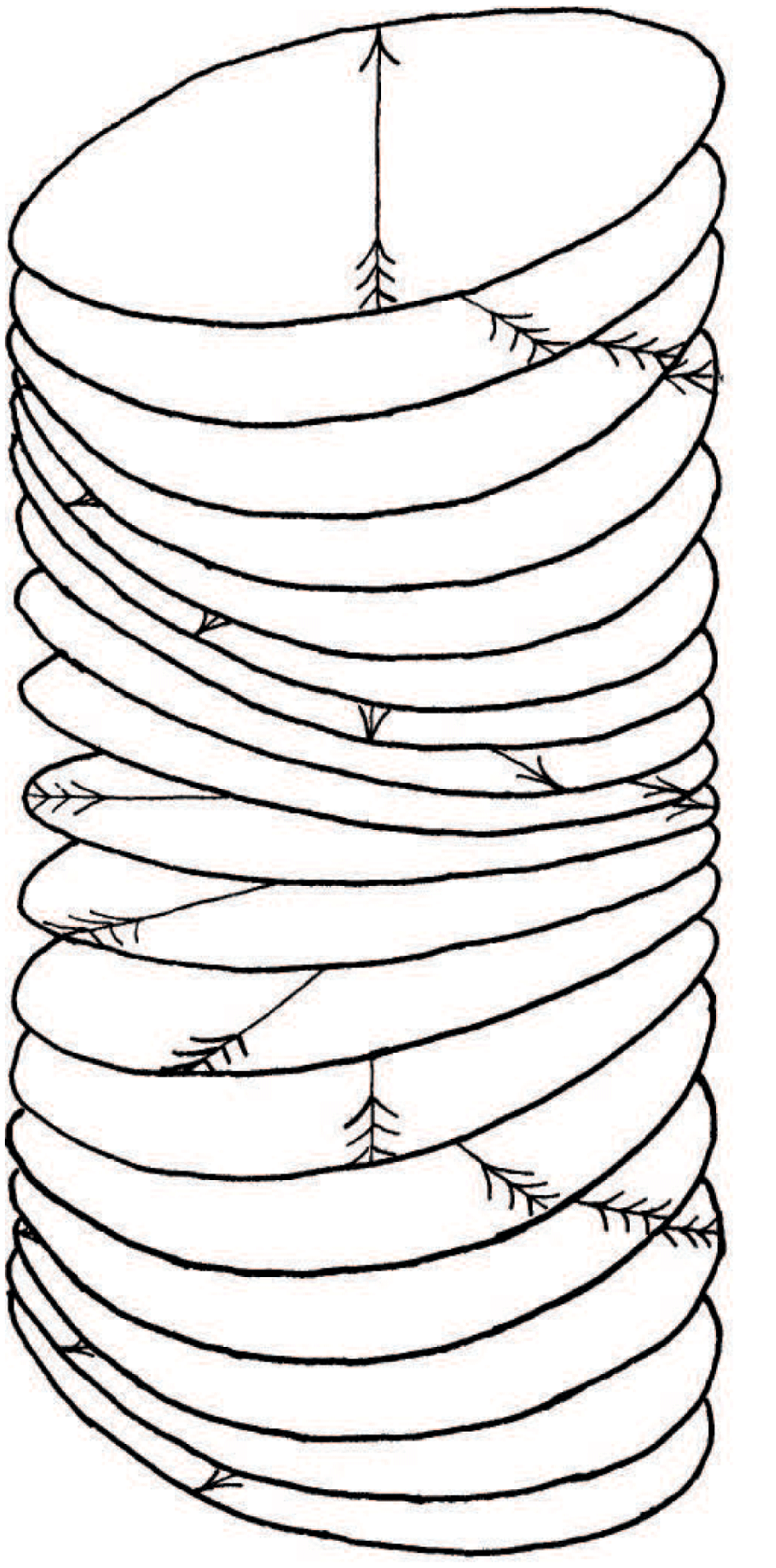
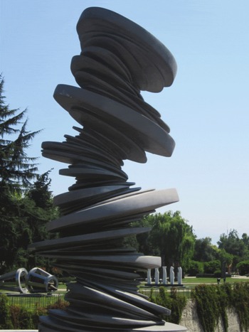
Thurston (Reference Thurston1972) described the Godbillon–Vey invariant as the wobble of a foliation or a pyramid of discs lying on top of each other (see figure 1). A similar wobble can be seen in the sculpture illustrated in figure 2 (from the Ghys (Reference Ghys2014) lecture on ‘Foliations: What’s next after Thurston’).
Illustrating the wobble of the foliations described by the Godbillon–Vey invariant (from Thurston (Reference Thurston1972) AMS vol. 76 (4), July 1972, 511–514).

The meaning of ‘wobble’ used above is presumably related to the wobble of spinning objects, due to the tilt between the axis of symmetry and its angular momentum (this in solid body dynamics involves the moments of inertia of the spinning body and the rotation axis of spin). A description of this phenomenon for rigid bodies is quite complicated (see e.g. Goldstein (Reference Goldstein1980), Marsden & Ratiu (Reference Marsden and Ratiu1994), Holm (Reference Holm2008), chap. 15, and also the webpage http:/www/mathpages.com/home/kmath/kmath116.htm).
3.3 Reinhart & Wood (Reference Reinhart and Wood1973) formula for Godbillon–Vey invariant
Reinhart & Wood (Reference Reinhart and Wood1973) (see also appendix E) show that the Godbillon–Vey invariant can be written in the form
 $$\begin{eqnarray}H_{\text{gv}}^{RW}=\int _{V_{g}}\hat{\unicode[STIX]{x1D702}}\wedge \text{d}\hat{\unicode[STIX]{x1D702}}=\int _{V_{g}}\unicode[STIX]{x1D705}^{2}(\unicode[STIX]{x1D70F}-h_{BN})\,\text{d}^{3}x,\end{eqnarray}$$
where
 $\unicode[STIX]{x1D705}$
and
 $\unicode[STIX]{x1D70F}$
are the curvature and torsion of a curve (or family of curves) with tangent vector
 $\boldsymbol{T}=\hat{\boldsymbol{A}}$
normal to the foliation (here
 $\hat{\unicode[STIX]{x1D6C8}}=\hat{\boldsymbol{A}}\times (\unicode[STIX]{x1D735}\times \hat{\boldsymbol{A}})=-\hat{\boldsymbol{A}}\boldsymbol{\cdot }\unicode[STIX]{x1D735}\hat{\boldsymbol{A}}=-\boldsymbol{k}$
where
 $\boldsymbol{k}$
is the curvature vector of the curve). The parameter
 $h_{ij}$
(
 $i,j=1,2$
) defines the second fundamental form for the surface, which describes the curvature of the foliation surface
 $\unicode[STIX]{x1D6F7}=\text{const}.$
Here
 $\boldsymbol{T},\boldsymbol{N},\boldsymbol{B}$
is the moving tri-hedron for the curve normal to the foliation, with tangent vector
 $\boldsymbol{T}$
, principal normal
 $\boldsymbol{N}$
and bi-normal
 $\boldsymbol{B}$
. These vector fields are governed by the Serret–Frenet formulae (or suitable equivalent formulae), and we use the notation
 $\boldsymbol{T}=\boldsymbol{e}_{3}$
,
 $\boldsymbol{N}=\boldsymbol{e}_{1}$
and
 $\boldsymbol{B}=\boldsymbol{e}_{2}$
for the orthonormal moving tri-hedron
 $\boldsymbol{T},\boldsymbol{N},\boldsymbol{B}$
, so that
 $h_{21}=h_{BN}$
. The main point of the Reinhart & Wood (Reference Reinhart and Wood1973) formula is that the curve with tangent vector
 $\boldsymbol{T}$
normal to the surface is a non-planar curve as it has both non-zero curvature (
 $\unicode[STIX]{x1D705}$
) and torsion (
 $\unicode[STIX]{x1D70F}$
), and it in general wobbles out of the original plane of the curve (for example if
 $h_{BN}$
is small then both
 $\unicode[STIX]{x1D705}$
and
 $\unicode[STIX]{x1D70F}$
must be non-zero in order for the differential invariant
 $\hat{\unicode[STIX]{x1D702}}\wedge \text{d}\hat{\unicode[STIX]{x1D702}}$
to be non-zero).
Illustrating the wobble of the foliations for a sculpture by Alejandra Ruddoff, used by Ghys (Reference Ghys2014) in his lecture on foliations (Ghys Reference Ghys2014).

Godbillon & Vey (Reference Godbillon and Vey1971) and Reinhart & Wood (Reference Reinhart and Wood1973), describe the Godbillon–Vey invariant for a co-dimension 1 foliation as a co-homology class defined by the three-form (3.11). This theory is important in algebraic topology in describing the topology of the distinct classes of closed curves that can be drawn on hypersurfaces in terms of the so-called Betti numbers and other topological invariants (see e.g. Pontryagin (Reference Pontryagin1952), Fulton (Reference Fulton1995) and Hatcher (Reference Hatcher2002)).
3.4 The MHD Godbillon–Vey field and invariant
The reason for the choice of
 $\unicode[STIX]{x1D6C8}$
in (3.10) is given below. The condition for the Pfaffian equation
 $\unicode[STIX]{x1D74E}_{A}^{1}=\boldsymbol{A}\boldsymbol{\cdot }\text{d}\boldsymbol{x}=0$
to be integrable defines a co-dimension 1 foliation, is that
 $$\begin{eqnarray}\boldsymbol{A}\boldsymbol{\cdot }(\unicode[STIX]{x1D735}\times \boldsymbol{A})\equiv \boldsymbol{A}\boldsymbol{\cdot }\boldsymbol{B}=0.\end{eqnarray}$$
In this case, the Pfaffian equation
 $\unicode[STIX]{x1D74E}_{A}^{1}=\boldsymbol{A}\boldsymbol{\cdot }\text{d}\boldsymbol{x}=0$
has an integrating factor
 $\unicode[STIX]{x1D707}$
such that
 $\unicode[STIX]{x1D707}\boldsymbol{A}=\unicode[STIX]{x1D735}\unicode[STIX]{x1D706}$
in which the foliation is described by the family of surfaces
 $\unicode[STIX]{x1D706}(x,y,z)=c_{1}$
. Each member of the family has unit normal
 $\hat{\boldsymbol{A}}=\boldsymbol{A}/|\boldsymbol{A}|^{2}$
(i.e. the normals to the surfaces are parallel to
 $\boldsymbol{A}$
). The integrability condition (3.14) can be expressed as
 $$\begin{eqnarray}\unicode[STIX]{x1D74E}_{A}^{1}\wedge \text{d}\unicode[STIX]{x1D74E}_{A}^{1}\equiv \boldsymbol{A}\boldsymbol{\cdot }\boldsymbol{B}\,\text{d}^{3}x=0.\end{eqnarray}$$
The condition (3.15) is satisfied if there exists a one-form
 $$\begin{eqnarray}\unicode[STIX]{x1D74E}_{\unicode[STIX]{x1D702}}^{1}=\unicode[STIX]{x1D6C8}\boldsymbol{\cdot }\text{d}\boldsymbol{x}\quad suchthat~\text{d}\unicode[STIX]{x1D74E}_{A}^{1}=\unicode[STIX]{x1D74E}_{\unicode[STIX]{x1D702}}^{1}\wedge \unicode[STIX]{x1D74E}_{A}^{1}.\end{eqnarray}$$
In that case,
 $$\begin{eqnarray}\unicode[STIX]{x1D74E}_{A}^{1}\wedge \text{d}\unicode[STIX]{x1D74E}_{A}^{1}=\unicode[STIX]{x1D74E}_{A}^{1}\wedge (\unicode[STIX]{x1D714}_{\unicode[STIX]{x1D702}}^{1}\wedge \unicode[STIX]{x1D74E}_{A}^{1})=0.\end{eqnarray}$$
Condition (3.16) can be written as
 $$\begin{eqnarray}\boldsymbol{B}\boldsymbol{\cdot }\text{d}\boldsymbol{S}=(\unicode[STIX]{x1D735}\times \boldsymbol{A})\boldsymbol{\cdot }\text{d}\boldsymbol{S}=(\unicode[STIX]{x1D6C8}\boldsymbol{\cdot }\text{d}\boldsymbol{x})\wedge (\boldsymbol{A}\boldsymbol{\cdot }\text{d}\boldsymbol{x})=(\unicode[STIX]{x1D6C8}\times \boldsymbol{A})\boldsymbol{\cdot }\text{d}\boldsymbol{S}.\end{eqnarray}$$
Equation (3.18) is satisfied if
 $$\begin{eqnarray}\boldsymbol{B}_{\bot }=\unicode[STIX]{x1D6C8}\times \boldsymbol{A}\quad \text{where}~\boldsymbol{B}_{\Vert }=\boldsymbol{B}\boldsymbol{\cdot }\hat{\boldsymbol{A}}\hat{\boldsymbol{A}}\text{ and }\boldsymbol{B}_{\bot }=\boldsymbol{B}-\boldsymbol{B}\boldsymbol{\cdot }\hat{\boldsymbol{A}}\hat{\boldsymbol{A}},\end{eqnarray}$$
where the subscripts
 $\Vert$
and
 $\bot$
denote components of
 $\boldsymbol{B}$
parallel and perpendicular to
 $\boldsymbol{A}$
. Taking the cross-product of
 $\boldsymbol{A}$
on the left with (3.19) gives
 $$\begin{eqnarray}\boldsymbol{A}\times \boldsymbol{B}_{\bot }=\boldsymbol{A}\times \boldsymbol{B}=\boldsymbol{A}\times (\unicode[STIX]{x1D6C8}\times \boldsymbol{A})=(\boldsymbol{A}\boldsymbol{\cdot }\boldsymbol{A})\unicode[STIX]{x1D6C8}-(\boldsymbol{A}\boldsymbol{\cdot }\unicode[STIX]{x1D6C8})\boldsymbol{A}.\end{eqnarray}$$
Choosing
 $\unicode[STIX]{x1D6C8}$
such that
 $\unicode[STIX]{x1D6C8}\boldsymbol{\cdot }\boldsymbol{A}=0$
, equation (3.20) gives
 $$\begin{eqnarray}\unicode[STIX]{x1D6C8}=\frac{\boldsymbol{A}\times \boldsymbol{B}}{|\boldsymbol{A}|^{2}}.\end{eqnarray}$$
This is the form of the Godbillon–Vey field that was adopted by Tur & Yanovsky (Reference Tur and Yanovsky1993) and Webb et al. (Reference Webb, Dasgupta, McKenzie, Hu and Zank2014a ). From (3.19) we obtain
 $$\begin{eqnarray}\boldsymbol{B}=\unicode[STIX]{x1D6FD}\boldsymbol{A}+\unicode[STIX]{x1D702}\times \boldsymbol{A}=\boldsymbol{B}_{\Vert }+\boldsymbol{B}_{\bot },\end{eqnarray}$$
where
 $$\begin{eqnarray}\unicode[STIX]{x1D6FD}=\frac{\boldsymbol{A}\boldsymbol{\cdot }\boldsymbol{B}}{|\boldsymbol{A}|^{2}}=\frac{h_{m}}{|\boldsymbol{A}|^{2}},\quad h_{m}=\boldsymbol{A}\boldsymbol{\cdot }\boldsymbol{B}.\end{eqnarray}$$
The formulae (3.21)–(3.23) play an essential role in the formulation of a transport equation for the Godbillon–Vey magnetic helicity for both the cases
 $h_{m}=0$
and
 $h_{m}\neq 0$
.
It is interesting to note that
 $$\begin{eqnarray}\boldsymbol{A}\times \boldsymbol{B}=\boldsymbol{A}\times (\unicode[STIX]{x1D735}\times \boldsymbol{A})=\unicode[STIX]{x1D735}\left({\textstyle \frac{1}{2}}|\boldsymbol{A}|^{2}\right)-\boldsymbol{A}\boldsymbol{\cdot }\unicode[STIX]{x1D735}\boldsymbol{A}.\end{eqnarray}$$
This result is analogous to the
 $\boldsymbol{J}\times \boldsymbol{B}$
force on the plasma, except that
 $\boldsymbol{B}$
has been replaced by
 $\boldsymbol{A}$
and there is a sign change. The first term is analogous to the gradient of a uniform pressure gradient of
 $A^{2}$
and the second term is analogous to the tension force of the magnetic field in the
 $\boldsymbol{J}\times \boldsymbol{B}$
force.
However, if we use normalized base vectors (i.e. unit vectors
 $\hat{\boldsymbol{A}}=\boldsymbol{A}/A$
) to describe the field, then we obtain
 $$\begin{eqnarray}\unicode[STIX]{x1D6C8}=\frac{\boldsymbol{A}\times \boldsymbol{B}}{|\boldsymbol{A}|^{2}}=\frac{A\unicode[STIX]{x1D735}A}{A^{2}}-\frac{A\hat{\boldsymbol{A}}\boldsymbol{\cdot }\unicode[STIX]{x1D735}(A\hat{\boldsymbol{A}})}{A^{2}}=(\unicode[STIX]{x1D644}-\hat{\boldsymbol{A}}\hat{\boldsymbol{A}})\boldsymbol{\cdot }\unicode[STIX]{x1D735}[\ln (A)]-\hat{\boldsymbol{A}}\boldsymbol{\cdot }\unicode[STIX]{x1D735}\hat{\boldsymbol{A}}.\end{eqnarray}$$
The first term in (3.25) is the gradient of
 $\ln (A)$
perpendicular to
 $\boldsymbol{A}$
and the second term is minus the curvature vector of
 $\hat{\boldsymbol{A}}$
. The
 $\boldsymbol{A}$
field line curvature term in (3.25) can be written in the form
 $$\begin{eqnarray}-\hat{\boldsymbol{A}}\boldsymbol{\cdot }\unicode[STIX]{x1D735}\hat{\boldsymbol{A}}=-\unicode[STIX]{x1D705}^{(A)}\boldsymbol{n}^{(A)},\end{eqnarray}$$
where
 $\boldsymbol{n}^{(A)}$
is the principal normal to the
 $\boldsymbol{A}$
field lines, and
 $\unicode[STIX]{x1D705}^{(A)}$
is the curvature of the
 $\boldsymbol{A}$
field lines;
 $\hat{\boldsymbol{A}}$
can be thought of as the tangent vector to a curve with principal normal
 $\boldsymbol{n}^{(A)}$
pointed towards the centre of curvature of the
 $\hat{\boldsymbol{A}}$
field (e.g. Lipschutz Reference Lipschutz1969).
3.5 Gauge transformations
For the case
 $\boldsymbol{A}\boldsymbol{\cdot }\boldsymbol{B}=0$
, equation (3.25) for
 $\unicode[STIX]{x1D6C8}$
implies
 $\unicode[STIX]{x1D6C8}\boldsymbol{\cdot }\boldsymbol{A}=\unicode[STIX]{x1D6C8}\boldsymbol{\cdot }\boldsymbol{B}=0$
. Thus,
 $\boldsymbol{A}$
,
 $\boldsymbol{B}$
and
 $\unicode[STIX]{x1D6C8}$
are mutually orthogonal vectors, in which
 $\boldsymbol{A}$
is normal to the foliation
 $\unicode[STIX]{x1D706}=\text{const}.$
Note that
 $$\begin{eqnarray}\unicode[STIX]{x1D707}\boldsymbol{A}\boldsymbol{\cdot }\text{d}\boldsymbol{x}=\text{d}\unicode[STIX]{x1D706}=\unicode[STIX]{x1D735}\unicode[STIX]{x1D706}\boldsymbol{\cdot }\text{d}\boldsymbol{x},\end{eqnarray}$$
where
 $\unicode[STIX]{x1D707}$
is an integrating factor. It is necessary to keep in mind that the use of
 $\boldsymbol{A}$
in (3.27) depends on the gauge for
 $\boldsymbol{A}$
. If for example,
 $\tilde{\boldsymbol{A}}=\boldsymbol{A}+\unicode[STIX]{x1D735}\unicode[STIX]{x1D719}$
, this will induce a change in the function
 $\unicode[STIX]{x1D706}$
. In other words, equation (3.27) in the new gauge leads to the equation
 $\tilde{\unicode[STIX]{x1D707}}\tilde{\boldsymbol{A}}\boldsymbol{\cdot }\text{d}\boldsymbol{x}=\text{d}\tilde{\unicode[STIX]{x1D706}}$
. If we fix the gauge of
 $\boldsymbol{A}$
, then the solution of (3.27) is
 $$\begin{eqnarray}\boldsymbol{A}=\unicode[STIX]{x1D708}\unicode[STIX]{x1D735}\unicode[STIX]{x1D706},\end{eqnarray}$$
where
 $\unicode[STIX]{x1D708}=1/\unicode[STIX]{x1D707}$
and
 $\unicode[STIX]{x1D707}$
is the integrating factor for the Pfaffian equation
 $\boldsymbol{A}\boldsymbol{\cdot }\text{d}\boldsymbol{x}=0$
. In this case the vectors
 $\unicode[STIX]{x1D6C8}$
,
 $\boldsymbol{B}$
lie in the
 $\unicode[STIX]{x1D706}=\text{const}.$
surface and
 $\boldsymbol{A}$
is normal to the surface (i.e.
 $\boldsymbol{N}\equiv \hat{\boldsymbol{A}}=\unicode[STIX]{x1D735}\unicode[STIX]{x1D706}/|\unicode[STIX]{x1D735}\unicode[STIX]{x1D706}|$
is the unit normal to the surface). The geometrical configuration of
 $\boldsymbol{A}$
,
 $\boldsymbol{B}$
and
 $\unicode[STIX]{x1D6C8}$
and the surface
 $\unicode[STIX]{x1D706}=\text{const}.$
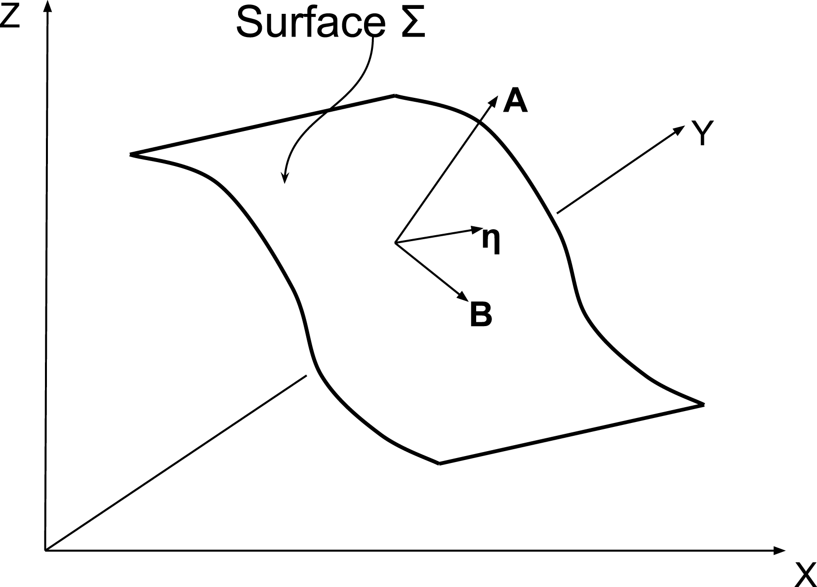
are depicted schematically in figure 3. Note that the vectors
 $\boldsymbol{A}$
,
 $\boldsymbol{B}$
and
 $\unicode[STIX]{x1D6C8}$
are mutually orthogonal, and with
 $\boldsymbol{B}$
and
 $\unicode[STIX]{x1D6C8}$
lying within the surface
 $\unicode[STIX]{x1D706}=\text{const}.$
The
 $\boldsymbol{B}$
surface
 $\unicode[STIX]{x1D6F4}$
with normal
 $\boldsymbol{A}$
and Godbillon–Vey field
 $\unicode[STIX]{x1D6C8}$
, where
 $\boldsymbol{A}\boldsymbol{\cdot }\boldsymbol{B}=0$
and
 $\unicode[STIX]{x1D6C8}=\boldsymbol{A}\times \boldsymbol{B}/A^{2}$
. Both
 $\boldsymbol{B}$
and
 $\unicode[STIX]{x1D6C8}$
are in the surface
 $\unicode[STIX]{x1D6F4}$
.

The magnetic vector potential
 $\boldsymbol{A}$
can admit a gauge potential transformation
 $\tilde{\boldsymbol{A}}=\boldsymbol{A}+\unicode[STIX]{x1D735}\unicode[STIX]{x1D719}$
, i.e.
 $$\begin{eqnarray}\tilde{\boldsymbol{A}}=\tilde{\unicode[STIX]{x1D708}}\unicode[STIX]{x1D735}\tilde{\unicode[STIX]{x1D706}}=\boldsymbol{A}+\unicode[STIX]{x1D735}\unicode[STIX]{x1D719}=\unicode[STIX]{x1D708}\unicode[STIX]{x1D735}\unicode[STIX]{x1D706}+\unicode[STIX]{x1D735}\unicode[STIX]{x1D719}\quad \text{where}~\boldsymbol{B}=\unicode[STIX]{x1D735}\times \boldsymbol{A}.\end{eqnarray}$$
In this case we obtain
 $$\begin{eqnarray}\tilde{\boldsymbol{A}}\boldsymbol{\cdot }\boldsymbol{B}=(\unicode[STIX]{x1D708}\unicode[STIX]{x1D735}\unicode[STIX]{x1D706}+\unicode[STIX]{x1D735}\unicode[STIX]{x1D719})\boldsymbol{\cdot }(\unicode[STIX]{x1D735}\unicode[STIX]{x1D708}\times \unicode[STIX]{x1D735}\unicode[STIX]{x1D706})=\unicode[STIX]{x1D735}\unicode[STIX]{x1D719}\boldsymbol{\cdot }(\unicode[STIX]{x1D735}\unicode[STIX]{x1D708}\times \unicode[STIX]{x1D735}\unicode[STIX]{x1D706})=J=\frac{\unicode[STIX]{x2202}(\unicode[STIX]{x1D719},\unicode[STIX]{x1D708},\unicode[STIX]{x1D706})}{\unicode[STIX]{x2202}(x,y,z)}.\end{eqnarray}$$
The zero Jacobian case
 $J=0$
or
 $\boldsymbol{A}\boldsymbol{\cdot }\boldsymbol{B}=0$
implies that
 $$\begin{eqnarray}\unicode[STIX]{x1D719}=\unicode[STIX]{x1D719}(\unicode[STIX]{x1D708},\unicode[STIX]{x1D706})\quad \text{for}~J=0.\end{eqnarray}$$
The gauge transformations (3.29) are discussed in appendix D.
If
 $\unicode[STIX]{x1D719}$
has discontinuous jumps across some surface, the integral of
 $\boldsymbol{A}\boldsymbol{\cdot }\boldsymbol{B}$
over a volume containing the discontinuity surface leads to a non-zero magnetic helicity integral over the volume. This implies that there is not a global single valued, smooth magnetic vector potential for
 $\boldsymbol{A}$
, and that a complicated magnetic field topology can arise due to the discontinuity surface for
 $\boldsymbol{A}$
. This possibility is used by Semenov et al. (Reference Semenov, Korovinski and Biernat2002) to describe the MHD topological soliton using Euler potentials.
In the case
 $\boldsymbol{A}\boldsymbol{\cdot }\boldsymbol{B}\neq 0$
, the space is not foliated into a family of surfaces. One could use Boozer coordinates (Boozer Reference Boozer1983, Reference Boozer2004) to describe the magnetic field, in which case we write
 $$\begin{eqnarray}\boldsymbol{A}=\unicode[STIX]{x1D708}\unicode[STIX]{x1D735}\unicode[STIX]{x1D706}+\unicode[STIX]{x1D713}\unicode[STIX]{x1D735}\unicode[STIX]{x1D719}\quad \text{and}\quad \boldsymbol{B}=\unicode[STIX]{x1D735}\unicode[STIX]{x1D708}\times \unicode[STIX]{x1D735}\unicode[STIX]{x1D706}+\unicode[STIX]{x1D735}\unicode[STIX]{x1D713}\times \unicode[STIX]{x1D735}\unicode[STIX]{x1D719}.\end{eqnarray}$$
The Clebsch representations (3.28)–(3.32) for the Godbillon–Vey helicity density
 $H_{\text{gv}}$
are discussed in appendix C.
3.6 Godbillon–Vey conservation law
Proposition 3.1. Using the advected
 $\boldsymbol{A}$
gauge in which the electric field potential
 $\unicode[STIX]{x1D713}=\boldsymbol{A}\boldsymbol{\cdot }\boldsymbol{u}$
(Gordin & Petviashvili Reference Gordin and Petviashvili1987, Reference Gordin and Petviashvili1989), the Godbillon–Vey helicity density
 $h_{\text{gv}}=\unicode[STIX]{x1D6C8}\boldsymbol{\cdot }(\unicode[STIX]{x1D735}\times \unicode[STIX]{x1D6C8})$
for MHD flows in which
 $\boldsymbol{A}\boldsymbol{\cdot }\boldsymbol{B}=0$
satisfies the conservation law
 $$\begin{eqnarray}\frac{\unicode[STIX]{x2202}h_{\text{gv}}}{\unicode[STIX]{x2202}t}+\unicode[STIX]{x1D735}\boldsymbol{\cdot }[\boldsymbol{u}h_{\text{gv}}+\unicode[STIX]{x1D6FC}\boldsymbol{B}]=0,\end{eqnarray}$$
where
 $$\begin{eqnarray}\displaystyle \left.\begin{array}{@{}c@{}}\displaystyle \unicode[STIX]{x1D6C8}=\frac{\boldsymbol{A}\times \boldsymbol{B}}{|\boldsymbol{A}|^{2}},\quad h_{\text{gv}}=\unicode[STIX]{x1D6C8}\boldsymbol{\cdot }(\unicode[STIX]{x1D735}\times \unicode[STIX]{x1D6C8}),\\ \displaystyle \unicode[STIX]{x1D6FC}=\frac{2\boldsymbol{A}\boldsymbol{\cdot }\unicode[STIX]{x03C3}\boldsymbol{\cdot }\unicode[STIX]{x1D6C8}}{|\boldsymbol{A}|^{2}}\equiv \frac{\boldsymbol{A}\boldsymbol{\cdot }\unicode[STIX]{x03C3}\boldsymbol{\cdot }\unicode[STIX]{x1D6C8}+\unicode[STIX]{x1D6C8}\boldsymbol{\cdot }\unicode[STIX]{x03C3}\boldsymbol{\cdot }\boldsymbol{A}}{|\boldsymbol{A}|^{2}},\\ \displaystyle \unicode[STIX]{x03C3}={\textstyle \frac{1}{2}}\left[\unicode[STIX]{x1D735}\boldsymbol{u}+(\unicode[STIX]{x1D735}\boldsymbol{u})^{T}-{\textstyle \frac{2}{3}}(\unicode[STIX]{x1D735}\boldsymbol{\cdot }\boldsymbol{u})\unicode[STIX]{x1D644}\right].\end{array}\right\} & & \displaystyle\end{eqnarray}$$
Here,
 $\unicode[STIX]{x1D6FC}$
depends on the shear tensor of the fluid
 $\unicode[STIX]{x03C3}$
. It describes the coupling of the fields
 $\boldsymbol{A}$
and
 $\unicode[STIX]{x1D6C8}$
due to shear in the flow. For shear-free flows,
 $\unicode[STIX]{x1D6FC}=0$
. The Godbillon–Vey helicity
 $H_{\text{gv}}=\int _{V_{m}}h_{\text{gv}}\,\text{d}^{3}x$
for a volume
 $V_{m}$
moving with the flow is conserved, i.e.
 $\text{d}H_{\text{gv}}/\text{d}t=0$
where it is assumed that
 $\boldsymbol{B}\boldsymbol{\cdot }\boldsymbol{n}=0$
on the boundary
 $\unicode[STIX]{x2202}V_{m}$
of
 $V_{m}$
.
Proof. The detailed proof follows as a consequence of the analysis of Tur & Yanovsky (Reference Tur and Yanovsky1993) and Webb et al. (Reference Webb, Dasgupta, McKenzie, Hu and Zank2014a ). A proof is given in appendix A.
4 Godbillon–Vey helicity for
 $\boldsymbol{A}\boldsymbol{\cdot }\boldsymbol{B}\neq 0$

In this section, we generalize the Godbillon–Vey helicity transport equation in two ways, namely (i) we determine the form of the transport equation for the case where the magnetic helicity
 $h_{m}=\boldsymbol{A}\boldsymbol{\cdot }\boldsymbol{B}\neq 0$
and (ii) we allow for a general electric field potential
 $\unicode[STIX]{x1D713}$
(i.e. we allow for more general gauges for
 $\boldsymbol{A}$
, other than the advected
 $\boldsymbol{A}$
gauge for which
 $\unicode[STIX]{x1D713}=\boldsymbol{A}\boldsymbol{\cdot }\boldsymbol{u}$
). The underlying idea is that Faraday’s equation for
 $\boldsymbol{B}$
can be split up into components parallel and perpendicular to
 $\boldsymbol{A}$
as in (3.22), i.e.
 $\boldsymbol{B}=\boldsymbol{B}_{\Vert }+\boldsymbol{B}_{\bot }$
, in which
 $\boldsymbol{B}_{\Vert }=h_{m}\boldsymbol{A}/|\boldsymbol{A}|^{2}$
, where
 $h_{m}=\boldsymbol{A}\boldsymbol{\cdot }\boldsymbol{B}$
, and
 $\boldsymbol{B}_{\bot }$
is related to the Godbillon–Vey field
 $\boldsymbol{\unicode[STIX]{x1D702}}=\boldsymbol{A}\times \boldsymbol{B}/|\boldsymbol{A}|^{2}$
by the formula
 $\boldsymbol{B}_{\bot }=\unicode[STIX]{x1D6C8}\times \boldsymbol{A}$
.
Proposition 4.1. The transport equation for the Godbillon–Vey helicity
 $h_{\text{gv}}=\unicode[STIX]{x1D6C8}\boldsymbol{\cdot }(\unicode[STIX]{x1D735}\times \unicode[STIX]{x1D6C8})$
where
 $\unicode[STIX]{x1D6C8}=\boldsymbol{A}\times \boldsymbol{B}/|\boldsymbol{A}|^{2}$
, for the general case where
 $h_{m}=\boldsymbol{A}\boldsymbol{\cdot }\boldsymbol{B}\neq 0$
, and for a general gauge for
 $\boldsymbol{A}$
has the form
 $$\begin{eqnarray}\frac{\unicode[STIX]{x2202}h_{\text{gv}}}{\unicode[STIX]{x2202}t}+\unicode[STIX]{x1D735}\boldsymbol{\cdot }(h_{\text{gv}}\boldsymbol{u})=Q,\end{eqnarray}$$
where the source term
 $Q$
in (4.1) is given by
 $$\begin{eqnarray}\displaystyle \left.\begin{array}{@{}c@{}}\displaystyle Q=\boldsymbol{S}\boldsymbol{\cdot }\unicode[STIX]{x1D735}\times \unicode[STIX]{x1D6C8}+\unicode[STIX]{x1D6C8}\boldsymbol{\cdot }\unicode[STIX]{x1D735}\times \boldsymbol{S},\\ \displaystyle \boldsymbol{S}=\frac{h_{m}}{|\boldsymbol{A}|^{4}}\boldsymbol{A}\times (2\unicode[STIX]{x03C3}\boldsymbol{\cdot }\boldsymbol{A}+\unicode[STIX]{x1D735}\unicode[STIX]{x1D701})+\frac{\boldsymbol{A}\boldsymbol{\cdot }\unicode[STIX]{x1D735}\unicode[STIX]{x1D701}}{|\boldsymbol{A}|^{2}}\unicode[STIX]{x1D6C8}+\unicode[STIX]{x1D6FC}\boldsymbol{A},\\ \displaystyle \unicode[STIX]{x1D6FC}=\frac{(2\boldsymbol{A}\boldsymbol{\cdot }\unicode[STIX]{x03C3}\boldsymbol{\cdot }\unicode[STIX]{x1D6C8}+\unicode[STIX]{x1D6C8}\boldsymbol{\cdot }\unicode[STIX]{x1D735}\unicode[STIX]{x1D701})}{|\boldsymbol{A}|^{2}},\quad \unicode[STIX]{x1D701}=\unicode[STIX]{x1D713}-\boldsymbol{A}\boldsymbol{\cdot }\boldsymbol{u},\end{array}\right\} & & \displaystyle\end{eqnarray}$$
and
 $\unicode[STIX]{x03C3}$
is the fluid velocity shear tensor in (3.34). Here,
 $\boldsymbol{S}$
is the source term in the Godbillon–Vey field evolution equation
 $$\begin{eqnarray}\unicode[STIX]{x1D6C8}_{t}-\boldsymbol{u}\times (\unicode[STIX]{x1D735}\times \unicode[STIX]{x1D6C8})+\unicode[STIX]{x1D735}(\boldsymbol{u}\boldsymbol{\cdot }\unicode[STIX]{x1D6C8})=\boldsymbol{S}.\end{eqnarray}$$
In the special case
 $\boldsymbol{A}\boldsymbol{\cdot }\boldsymbol{B}=0$
and
 $\unicode[STIX]{x1D701}=0$
(
 $\unicode[STIX]{x1D713}=\boldsymbol{A}\boldsymbol{\cdot }\boldsymbol{u}$
) the Godbillon–Vey transport equation (4.1) reduces to the conservation law (3.33). In the advected
 $\boldsymbol{A}$
gauge (
 $\unicode[STIX]{x1D701}=0$
and
 $\unicode[STIX]{x1D713}=\boldsymbol{A}\boldsymbol{\cdot }\boldsymbol{u}$
), equation (4.2) gives the simplified formulae
 $$\begin{eqnarray}\boldsymbol{S}=\boldsymbol{S}^{0}=\frac{2h_{m}}{|\boldsymbol{A}|^{4}}\boldsymbol{A}\times (\unicode[STIX]{x03C3}\boldsymbol{\cdot }\boldsymbol{A})+\unicode[STIX]{x1D6FC}\boldsymbol{A},\quad \unicode[STIX]{x1D6FC}\equiv \unicode[STIX]{x1D6FC}_{0}=\frac{2(\boldsymbol{A}\boldsymbol{\cdot }\unicode[STIX]{x03C3}\boldsymbol{\cdot }\unicode[STIX]{x1D6C8})}{|\boldsymbol{A}|^{2}}.\end{eqnarray}$$
Proof. The proof is given in appendix B.
5 The Low & Lou (Reference Low and Lou1990) force-free magnetic fields
In this section we investigate the Godbillon–Vey helicity of the Low & Lou (Reference Low and Lou1990) force-free magnetic fields. Both Low & Lou (Reference Low and Lou1990) and Prasad et al. (Reference Prasad, Mangalam and Ravindra2014) used these fields to discuss solar photospheric magnetic fields. Prasad et al. (Reference Prasad, Mangalam and Ravindra2014) investigated models of force-free magnetic fields in order to describe solar magnetic fields observed by the Hinode spectro-polarimeter. They studied the relative magnetic helicity and magnetic free energy of magnetically active regions on the Sun, both before and after solar flares.
The force-free magnetic fields arise in low beta magnetic fields in a highly conducting plasma when the dominant force in the magneto-static force balance is the
 $\boldsymbol{J}\times \boldsymbol{B}$
force. In this case, the approximate force balance equation reduces to
 $\boldsymbol{J}\times \boldsymbol{B}=(\unicode[STIX]{x1D735}\times \boldsymbol{B})\times \boldsymbol{B}/\unicode[STIX]{x1D707}_{0}=0$
. For force-free fields,
 $\boldsymbol{B}$
is to lowest order parallel to the current
 $\boldsymbol{J}$
so that
 $$\begin{eqnarray}\unicode[STIX]{x1D735}\times \boldsymbol{B}=\unicode[STIX]{x1D6FC}\boldsymbol{B},\quad \unicode[STIX]{x1D735}\boldsymbol{\cdot }\boldsymbol{B}=0,\quad \boldsymbol{B}\boldsymbol{\cdot }\unicode[STIX]{x1D735}\unicode[STIX]{x1D6FC}=0.\end{eqnarray}$$
For linear force-free fields
 $\unicode[STIX]{x1D6FC}$
is taken to be constant (e.g. Chandrasekhar Reference Chandrasekhar1956). For nonlinear force-free fields, the function
 $\unicode[STIX]{x1D6FC}$
can be a nonlinear function of the magnetic vector potential
 $\boldsymbol{A}$
, or of a component of
 $\boldsymbol{A}$
. From (5.1) we obtain the condition
 $$\begin{eqnarray}\unicode[STIX]{x1D735}\boldsymbol{\cdot }(\unicode[STIX]{x1D735}\times \boldsymbol{B})=\unicode[STIX]{x1D735}\boldsymbol{\cdot }(\unicode[STIX]{x1D6FC}\boldsymbol{B})=\boldsymbol{B}\boldsymbol{\cdot }\unicode[STIX]{x1D735}\unicode[STIX]{x1D6FC}=0.\end{eqnarray}$$
Thus
 $\unicode[STIX]{x1D6FC}$
is constant along a field line.
The nonlinear force-free magnetic fields of Low & Lou (Reference Low and Lou1990) have the form
 $$\begin{eqnarray}\boldsymbol{B}=\unicode[STIX]{x1D735}\unicode[STIX]{x1D713}\times \unicode[STIX]{x1D735}\unicode[STIX]{x1D719}+\frac{Q\boldsymbol{e}_{\unicode[STIX]{x1D719}}}{r\sin \unicode[STIX]{x1D703}}\equiv \frac{\unicode[STIX]{x1D735}\unicode[STIX]{x1D713}\times \boldsymbol{e}_{\unicode[STIX]{x1D719}}+Q\boldsymbol{e}_{\unicode[STIX]{x1D719}}}{r\sin \unicode[STIX]{x1D703}},\end{eqnarray}$$
where
 $(r,\unicode[STIX]{x1D703},\unicode[STIX]{x1D719})$
are spherical polar coordinates, and
 $$\begin{eqnarray}\boldsymbol{e}_{r}=\frac{\unicode[STIX]{x2202}\boldsymbol{r}}{\unicode[STIX]{x2202}r},\quad \boldsymbol{e}_{\unicode[STIX]{x1D703}}=\frac{1}{r}\frac{\unicode[STIX]{x2202}\boldsymbol{r}}{\unicode[STIX]{x2202}\unicode[STIX]{x1D703}},\quad \boldsymbol{e}_{\unicode[STIX]{x1D719}}=\frac{1}{r\sin \unicode[STIX]{x1D703}}\frac{\unicode[STIX]{x2202}\boldsymbol{r}}{\unicode[STIX]{x2202}\unicode[STIX]{x1D719}},\end{eqnarray}$$
are orthonormal unit vectors in the
 $r$
,
 $\unicode[STIX]{x1D703}$
and
 $\unicode[STIX]{x1D719}$
directions. In (5.3)
 $A=A(r,\unicode[STIX]{x1D703})$
and
 $Q=Q(r,\unicode[STIX]{x1D703})$
.
Using the magnetic field representation (5.3), (5.1) give the equations
 $$\begin{eqnarray}\displaystyle & \displaystyle \frac{1}{r^{2}\sin \unicode[STIX]{x1D703}}\left(\frac{\unicode[STIX]{x2202}Q}{\unicode[STIX]{x2202}\unicode[STIX]{x1D703}}-\unicode[STIX]{x1D6FC}\frac{\unicode[STIX]{x2202}\unicode[STIX]{x1D713}}{\unicode[STIX]{x2202}\unicode[STIX]{x1D703}}\right)=0, & \displaystyle\end{eqnarray}$$
 $$\begin{eqnarray}\displaystyle & \displaystyle \frac{1}{r\sin \unicode[STIX]{x1D703}}\left(-\frac{\unicode[STIX]{x2202}Q}{\unicode[STIX]{x2202}r}+\unicode[STIX]{x1D6FC}\frac{\unicode[STIX]{x2202}\unicode[STIX]{x1D713}}{\unicode[STIX]{x2202}r}\right)=0, & \displaystyle\end{eqnarray}$$
 $$\begin{eqnarray}\displaystyle & \displaystyle \frac{1}{r\sin \unicode[STIX]{x1D703}}\frac{\unicode[STIX]{x2202}^{2}\unicode[STIX]{x1D713}}{\unicode[STIX]{x2202}r^{2}}+\frac{1}{r^{3}}\frac{\unicode[STIX]{x2202}}{\unicode[STIX]{x2202}\unicode[STIX]{x1D703}}\left(\frac{1}{\sin \unicode[STIX]{x1D703}}\frac{\unicode[STIX]{x2202}\unicode[STIX]{x1D713}}{\unicode[STIX]{x2202}\unicode[STIX]{x1D703}}\right)+\frac{\unicode[STIX]{x1D6FC}Q}{r\sin \unicode[STIX]{x1D703}}=0, & \displaystyle\end{eqnarray}$$
as the components of the force balance equation in the
 $r$
,
 $\unicode[STIX]{x1D703}$
and
 $\unicode[STIX]{x1D719}$
directions respectively.
From (5.5) and (5.6) the compatibility condition
 $$\begin{eqnarray}\frac{\unicode[STIX]{x2202}\unicode[STIX]{x1D713}}{\unicode[STIX]{x2202}r}\left(\frac{\unicode[STIX]{x2202}Q}{\unicode[STIX]{x2202}\unicode[STIX]{x1D703}}-\unicode[STIX]{x1D6FC}\frac{\unicode[STIX]{x2202}\unicode[STIX]{x1D713}}{\unicode[STIX]{x2202}\unicode[STIX]{x1D703}}\right)-\frac{\unicode[STIX]{x2202}\unicode[STIX]{x1D713}}{\unicode[STIX]{x2202}\unicode[STIX]{x1D703}}\left(\frac{\unicode[STIX]{x2202}Q}{\unicode[STIX]{x2202}r}-\unicode[STIX]{x1D6FC}\frac{\unicode[STIX]{x2202}\unicode[STIX]{x1D713}}{\unicode[STIX]{x2202}r}\right)\equiv \frac{\unicode[STIX]{x2202}(Q,\unicode[STIX]{x1D713})}{\unicode[STIX]{x2202}(\unicode[STIX]{x1D703},r)}=0,\end{eqnarray}$$
implies
 $Q=Q(\unicode[STIX]{x1D713})$
. Similarly, the condition
 $\boldsymbol{B}\boldsymbol{\cdot }\unicode[STIX]{x1D735}\unicode[STIX]{x1D6FC}=0$
in (5.1) requires
 $$\begin{eqnarray}B_{r}\frac{\unicode[STIX]{x2202}\unicode[STIX]{x1D6FC}}{\unicode[STIX]{x2202}r}+\frac{B_{\unicode[STIX]{x1D703}}}{r}\frac{\unicode[STIX]{x2202}\unicode[STIX]{x1D6FC}}{\unicode[STIX]{x2202}\unicode[STIX]{x1D703}}\equiv \frac{1}{r^{2}\sin \unicode[STIX]{x1D703}}\frac{\unicode[STIX]{x2202}(\unicode[STIX]{x1D713},\unicode[STIX]{x1D6FC})}{\unicode[STIX]{x2202}(\unicode[STIX]{x1D703},r)}=0.\end{eqnarray}$$
Equation (5.9) requires that
 $\unicode[STIX]{x1D6FC}=\unicode[STIX]{x1D6FC}(\unicode[STIX]{x1D713})$
. Equations (5.5) and (5.6) give the equations
 $$\begin{eqnarray}\frac{\unicode[STIX]{x2202}\unicode[STIX]{x1D713}}{\unicode[STIX]{x2202}\unicode[STIX]{x1D703}}\left(\frac{\text{d}Q}{\text{d}\unicode[STIX]{x1D713}}-\unicode[STIX]{x1D6FC}\right)=0,\quad \frac{\unicode[STIX]{x2202}\unicode[STIX]{x1D713}}{\unicode[STIX]{x2202}r}\left(-\frac{\text{d}Q}{\text{d}\unicode[STIX]{x1D713}}+\unicode[STIX]{x1D6FC}\right)=0,\quad \text{and}\quad \unicode[STIX]{x1D6FC}=\frac{\text{d}Q}{\text{d}\unicode[STIX]{x1D713}}.\end{eqnarray}$$
Using
 $\unicode[STIX]{x1D6FC}=\text{d}Q/\text{d}\unicode[STIX]{x1D713}$
and
 $Q=Q(\unicode[STIX]{x1D713})$
in (5.7) gives the equation
 $$\begin{eqnarray}\frac{\unicode[STIX]{x2202}^{2}\unicode[STIX]{x1D713}}{\unicode[STIX]{x2202}r^{2}}+\frac{(1-\unicode[STIX]{x1D707}^{2})}{r^{2}}\frac{\unicode[STIX]{x2202}^{2}\unicode[STIX]{x1D713}}{\unicode[STIX]{x2202}\unicode[STIX]{x1D707}^{2}}+\frac{\text{d}Q(\unicode[STIX]{x1D713})}{\text{d}\unicode[STIX]{x1D713}}Q(\unicode[STIX]{x1D713})=0,\end{eqnarray}$$
where
 $\unicode[STIX]{x1D707}=\cos \unicode[STIX]{x1D703}$
. Thus, the nonlinear force-free magnetic field equation (5.1) reduces to the second-order partial differential equation (5.11) for
 $\unicode[STIX]{x1D713}$
, with ignorable spherical polar coordinate
 $\unicode[STIX]{x1D719}$
. Equation (5.11) is analogous to the Grad–Shafranov equation for MHD equilibria with ignorable coordinate
 $\unicode[STIX]{x1D719}$
.
From Low & Lou (Reference Low and Lou1990) and Prasad et al. (Reference Prasad, Mangalam and Ravindra2014), (5.11) admits separable solutions for
 $\unicode[STIX]{x1D713}$
of the form
 $$\begin{eqnarray}\unicode[STIX]{x1D713}=\frac{P(\unicode[STIX]{x1D707})}{r^{n}},\quad Q=a\unicode[STIX]{x1D713}^{1+1/n},\end{eqnarray}$$
where
 $a$
is a constant and
 $P(\unicode[STIX]{x1D707})$
satisfies the nonlinear second-order differential equation
 $$\begin{eqnarray}(1-\unicode[STIX]{x1D707}^{2})\frac{\text{d}^{2}P}{\text{d}\unicode[STIX]{x1D707}^{2}}+n(n+1)P+a^{2}\left(\frac{n+1}{n}\right)P^{1+2/n}=0.\end{eqnarray}$$
For
 $a=0$
, the solution of (5.13), which is regular at
 $\unicode[STIX]{x1D707}=\pm 1$
is
 $$\begin{eqnarray}P(\unicode[STIX]{x1D707})=(1-\unicode[STIX]{x1D707}^{2})^{1/2}P_{n}^{1}(\unicode[STIX]{x1D707}),\end{eqnarray}$$
where
 $P_{n}^{m}(\unicode[STIX]{x1D707})$
is Legendre’s associated function.
Here
 $a=0$
implies
 $Q=0$
and
 $\unicode[STIX]{x1D6FC}=0$
, which represent the potential field (untwisted) solutions. For the non-potential cases (
 $a\neq 0$
), the above nonlinear equation has to be solved numerically as an eigenvalue problem (for different values of
 $a$
) subject to the boundary conditions
 $P=0$
at
 $\unicode[STIX]{x1D707}=\pm 1$
. The solutions of (5.13) for the restrictive case of
 $n=1$
were presented in Low & Lou (Reference Low and Lou1990), which were constrained to due to an inherent singularity in
 $P$
at
 $\unicode[STIX]{x1D707}=0$
for higher values of
 $n$
. These solutions were later extended for higher odd values of
 $n$
by Prasad et al. (Reference Prasad, Mangalam and Ravindra2014) through the transformation
 $P(\unicode[STIX]{x1D707})=\sqrt{(}1-\unicode[STIX]{x1D707}^{2})F(\unicode[STIX]{x1D707})$
and then solving the (5.13) in terms of
 $F$
where
 $$\begin{eqnarray}(1-\unicode[STIX]{x1D707}^{2})\frac{\text{d}^{2}F}{\text{d}\unicode[STIX]{x1D707}^{2}}-2\unicode[STIX]{x1D707}\frac{\text{d}F}{\text{d}\unicode[STIX]{x1D707}}+\left[n(n+1)-\frac{1}{(1-\unicode[STIX]{x1D707}^{2})}\right]F(\unicode[STIX]{x1D707})+a^{2}\frac{(n+1)}{n}F^{(n+2)/n}(1-\unicode[STIX]{x1D707}^{2})^{1/n}=0,\end{eqnarray}$$
with the boundary conditions
 $F(\unicode[STIX]{x1D707})=0$
at
 $\unicode[STIX]{x1D707}=\pm 1$
.
Following Prasad et al. (Reference Prasad, Mangalam and Ravindra2014) we search for a two-dimensional magnetic vector potential of the form
 $$\begin{eqnarray}\boldsymbol{A}=A_{\unicode[STIX]{x1D703}}\boldsymbol{e}_{\unicode[STIX]{x1D703}}+A_{\unicode[STIX]{x1D719}}\boldsymbol{e}_{\unicode[STIX]{x1D719}},\end{eqnarray}$$
where
 $\boldsymbol{B}=\unicode[STIX]{x1D735}\times \boldsymbol{A}$
. Using (5.3), (5.12), (5.13) and (5.16) we obtain the equations
 $$\begin{eqnarray}\displaystyle \left.\begin{array}{@{}c@{}}\displaystyle B_{r}=\frac{1}{r\sin \unicode[STIX]{x1D703}}\left[\frac{\unicode[STIX]{x2202}}{\unicode[STIX]{x2202}\unicode[STIX]{x1D703}}(A_{\unicode[STIX]{x1D719}}\sin \unicode[STIX]{x1D703})-\frac{\unicode[STIX]{x2202}A_{\unicode[STIX]{x1D703}}}{\unicode[STIX]{x2202}\unicode[STIX]{x1D719}}\right]=-\frac{\text{d}P/\text{d}\unicode[STIX]{x1D707}}{r^{n+2}},\\ \displaystyle B_{\unicode[STIX]{x1D703}}=-\frac{1}{r}\frac{\unicode[STIX]{x2202}}{\unicode[STIX]{x2202}r}(rA_{\unicode[STIX]{x1D719}})=\frac{nP(\unicode[STIX]{x1D707})}{r^{n+2}\sin \unicode[STIX]{x1D703}},\\ \displaystyle B_{\unicode[STIX]{x1D719}}=\frac{1}{r}\frac{\unicode[STIX]{x2202}}{\unicode[STIX]{x2202}r}(rA_{\unicode[STIX]{x1D703}})=\frac{a[P(\unicode[STIX]{x1D707})]^{(n+1)/n}}{r^{n+2}\sin \unicode[STIX]{x1D703}}.\end{array}\right\} & & \displaystyle\end{eqnarray}$$
Integration of (5.17) gives the solutions
 $$\begin{eqnarray}A_{\unicode[STIX]{x1D703}}=-\frac{1}{n}\frac{a[P(\unicode[STIX]{x1D707})]^{(n+1)/n}}{r^{n+1}\sin \unicode[STIX]{x1D703}},\quad A_{\unicode[STIX]{x1D719}}=\frac{P(\unicode[STIX]{x1D707})}{r^{n+1}\sin \unicode[STIX]{x1D703}},\end{eqnarray}$$
for
 $A_{\unicode[STIX]{x1D703}}$
and
 $A_{\unicode[STIX]{x1D719}}$
.
Using (5.17) and (5.18) it follows that
 $$\begin{eqnarray}\boldsymbol{A}\boldsymbol{\cdot }\boldsymbol{B}=A_{\unicode[STIX]{x1D703}}B_{\unicode[STIX]{x1D703}}+A_{\unicode[STIX]{x1D719}}B_{\unicode[STIX]{x1D719}}=0.\end{eqnarray}$$
Thus
 $\boldsymbol{A}\boldsymbol{\cdot }\unicode[STIX]{x1D735}\times \boldsymbol{A}=0$
, which implies that the Pfaffian
 $\boldsymbol{A}\boldsymbol{\cdot }\text{d}\boldsymbol{x}=0$
admits an integrating factor,
 $\unicode[STIX]{x1D707}$
such that
 $\unicode[STIX]{x1D707}\boldsymbol{A}\boldsymbol{\cdot }\text{d}\boldsymbol{x}=\text{d}\unicode[STIX]{x1D6F7}$
where
 $\unicode[STIX]{x1D6F7}(\boldsymbol{x})=\text{const}.$
is a foliation with normal
 $\boldsymbol{A}$
. The magnetic field
 $\boldsymbol{B}$
and the Godbillon–Vey field
 $\unicode[STIX]{x1D6C8}=\boldsymbol{A}\times \boldsymbol{B}/|\boldsymbol{A}|^{2}$
lie on the foliation. Using (5.17)–(5.18), the components of
 $\unicode[STIX]{x1D6C8}$
are given by the equations
 $$\begin{eqnarray}\unicode[STIX]{x1D702}_{r}=-\frac{n}{r},\quad \unicode[STIX]{x1D702}_{\unicode[STIX]{x1D703}}=-\frac{(\text{d}P/\text{d}\unicode[STIX]{x1D707})\sin \unicode[STIX]{x1D703}}{rP[1+(a^{2}/n^{2})P^{2/n}]},\quad \unicode[STIX]{x1D702}_{\unicode[STIX]{x1D719}}=-\frac{aP^{(1/n-1)}(\text{d}P/\text{d}\unicode[STIX]{x1D707})\sin \unicode[STIX]{x1D703}}{nrP[1+(a^{2}/n^{2})P^{2/n}]}.\end{eqnarray}$$
In the evaluation of (5.20) we used the formula
 $$\begin{eqnarray}|\boldsymbol{A}|^{2}=\frac{[1+(a^{2}/n^{2})P^{2/n}]P^{2}}{r^{2n+2}\sin ^{2}\unicode[STIX]{x1D703}}.\end{eqnarray}$$
Calculating
 $\unicode[STIX]{x1D735}\times \unicode[STIX]{x1D6C8}$
we obtain
 $$\begin{eqnarray}(\unicode[STIX]{x1D735}\times \unicode[STIX]{x1D6C8})_{r}=\frac{a}{nr^{2}}\frac{\text{d}}{\text{d}\unicode[STIX]{x1D707}}\left(\frac{P^{(1/n-1)}(\text{d}P/\text{d}\unicode[STIX]{x1D707})(1-\unicode[STIX]{x1D707}^{2})}{[1+(a^{2}/n^{2})P^{2/n}]}\right),\quad (\unicode[STIX]{x1D735}\times \unicode[STIX]{x1D6C8})_{\unicode[STIX]{x1D703}}=(\unicode[STIX]{x1D735}\times \unicode[STIX]{x1D6C8})_{\unicode[STIX]{x1D719}}=0.\end{eqnarray}$$
Using (5.20)–(5.22) we obtain the Godbillon–Vey helicity density
 $h_{\unicode[STIX]{x1D702}}$
as
 $$\begin{eqnarray}h_{\unicode[STIX]{x1D702}}=\unicode[STIX]{x1D6C8}\boldsymbol{\cdot }\unicode[STIX]{x1D735}\times \unicode[STIX]{x1D6C8}=-\frac{a}{r^{3}}\frac{\text{d}}{\text{d}\unicode[STIX]{x1D707}}\left(\frac{P^{(1/n-1)}\text{d}P/\text{d}\unicode[STIX]{x1D707}(1-\unicode[STIX]{x1D707}^{2})}{[1+(a^{2}/n^{2})P^{2/n}]}\right).\end{eqnarray}$$
Note that for the potential field with
 $a=0$
, the Godbillon–Vey helicity density
 $h_{\text{gv}}\equiv h_{\unicode[STIX]{x1D702}}$
is zero. Only for
 $a\neq 0$
is there a non-zero Godbillon–Vey helicity. The parameter
 $a$
is an eigenvalue in the nonlinear force-free fields obtained by Low & Lou (Reference Low and Lou1990) and Prasad et al. (Reference Prasad, Mangalam and Ravindra2014). The eigenfunctions
 $P(\unicode[STIX]{x1D707})$
are characterized by the label
 $n$
(see (5.13)), which determines the radial dependence of the solution for
 $\unicode[STIX]{x1D713}$
. A similar classification applies to the
 $F(\unicode[STIX]{x1D707})$
, where
 $P(\unicode[STIX]{x1D707})=\sqrt{(1-\unicode[STIX]{x1D707}^{2})}$
. The eigenfunctions are also labelled by the index
 $m$
where
 $m=1$
corresponds to the lowest possible value of the eigenvalue
 $a$
that fits the boundary conditions
 $F(\unicode[STIX]{x1D707})=0$
at
 $\unicode[STIX]{x1D707}=\pm 1$
.
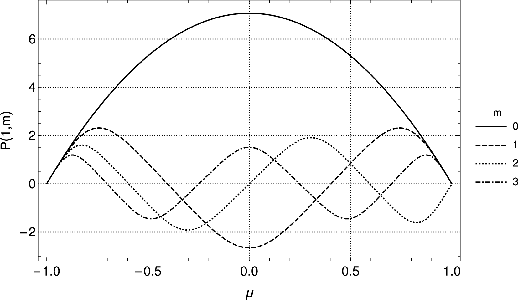
Low & Lou (Reference Low and Lou1990) force-free magnetic field eigenfunctions
 $P(n,m)$
for
 $n=1$
versus
 $\unicode[STIX]{x1D707}$
where
 $\unicode[STIX]{x1D707}=\cos \unicode[STIX]{x1D703}$
and
 $(r,\unicode[STIX]{x1D703},\unicode[STIX]{x1D719})$
are spherical polar coordinates.
 $m=0,1,2,3$
.

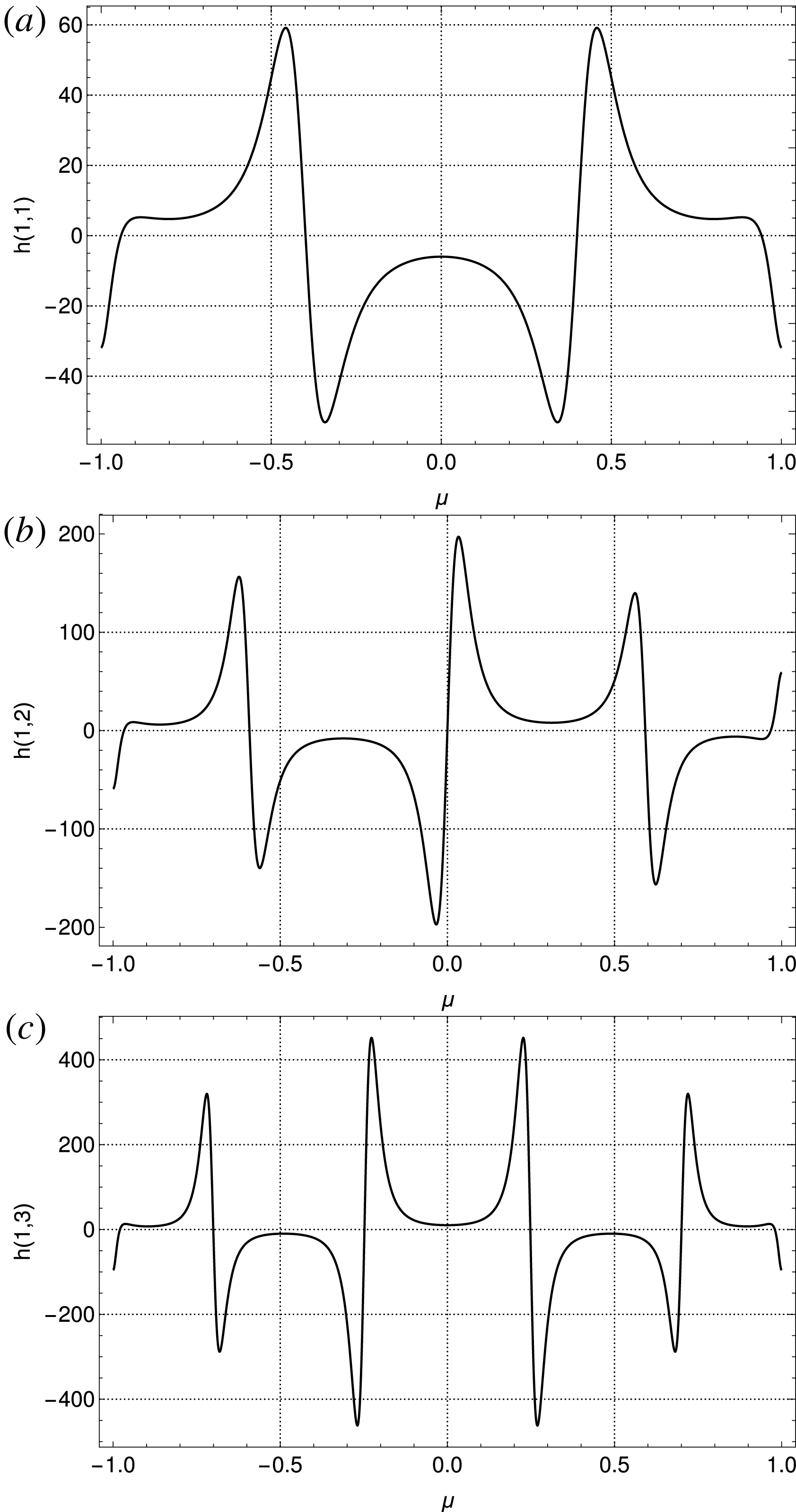
Figure 4 shows the eigenfunctions
 $P(n,m;\unicode[STIX]{x1D707})$
versus
 $\unicode[STIX]{x1D707}$
for
 $-1<\unicode[STIX]{x1D707}<1$
, for
 $n=1$
and
 $m=0,1,2,3$
. The case
 $m=0$
corresponds to the potential field case where
 $P(\unicode[STIX]{x1D707})=1-\unicode[STIX]{x1D707}^{2}$
. For
 $m=1$
and
 $m=3$
 $P(\unicode[STIX]{x1D707})$
is even in
 $\unicode[STIX]{x1D707}$
, but for
 $m=2$
,
 $P(\unicode[STIX]{x1D707})$
is odd in
 $\unicode[STIX]{x1D707}$
(see also Low & Lou (Reference Low and Lou1990) and Prasad et al. (Reference Prasad, Mangalam and Ravindra2014)).
Godbillon–Vey helicity density
 $h(n,m)$
versus
 $\unicode[STIX]{x1D707}$
for the Low & Lou (Reference Low and Lou1990) force-free magnetic field (5.17).
 $h(n,m)\equiv h_{\unicode[STIX]{x1D702}}$
is given by (5.23). The parameter
 $n=1$
and
 $m=1,2,3$
(a–c). Note
 $h(1,1)$
and
 $h(1,3)$
are even in
 $\unicode[STIX]{x1D707}$
but
 $h(1,2)$
(b) is odd in
 $\unicode[STIX]{x1D707}$
.

Figure 5 shows the Godbillon–Vey helicity
 $h\equiv h_{\unicode[STIX]{x1D702}}$
(equation (5.23) versus
 $\unicode[STIX]{x1D707}$
(
 $-1\leqslant \unicode[STIX]{x1D707}\leqslant 1$
) for
 $r=1$
, for
 $n=1$
and for
 $m=1,2,3$
. The panels corresponds to
 $m=1$
(a)
 $m=2$
(b) and
 $m=3$
(c). The helicity densities
 $h(1,m)$
versus
 $\unicode[STIX]{x1D707}$
are shown for
 $m=1,2,3$
from (a) to (c). For
 $m=1$
and
 $m=3$
the helicity densities
 $h(1,m)$
are even in
 $\unicode[STIX]{x1D707}$
but
 $h(1,2)$
for
 $m=2$
is odd in
 $\unicode[STIX]{x1D707}$
. Note the existence of positive and negative values of
 $h\equiv h_{\text{gv}}$
as a function of
 $\unicode[STIX]{x1D707}$
. The maximum and minimum values of
 $h$
increases with
 $m$
.
Cumulative Godbillon–Vey helicity
 $g(n,m)$
versus
 $\unicode[STIX]{x1D707}$
for the Low & Lou (Reference Low and Lou1990) force-free magnetic field (5.17).
 $g(n,m)\equiv g(\unicode[STIX]{x1D707})$
is given by (5.24). The parameter
 $n=1$
and
 $m=1,2,3$
(a–c). Note
 $g(1,1)$
and
 $g(1,3)$
are odd in
 $\unicode[STIX]{x1D707}$
but
 $g(1,2)$
(b) is even in
 $\unicode[STIX]{x1D707}$
.

Perhaps of more physical interest is the net Godbillon–Vey helicity integral for
 $r=1$
, namely
 $$\begin{eqnarray}g(\unicode[STIX]{x1D707})=\int _{\unicode[STIX]{x1D707}=-1}^{\unicode[STIX]{x1D707}}\text{d}\unicode[STIX]{x1D707}^{\prime }h_{\unicode[STIX]{x1D702}}(\unicode[STIX]{x1D707}^{\prime })=-a\left[\left(\frac{P^{(1/n-1)}(\unicode[STIX]{x1D707}^{\prime })\,\text{d}P(\unicode[STIX]{x1D707}^{\prime })/\text{d}\unicode[STIX]{x1D707}^{\prime }(1-\unicode[STIX]{x1D707}^{^{\prime }2})}{[1+(a^{2}/n^{2})P(\unicode[STIX]{x1D707}^{\prime })^{2/n}]}\right)\right]_{\unicode[STIX]{x1D707}^{\prime }=-1}^{\unicode[STIX]{x1D707}^{\prime }=\unicode[STIX]{x1D707}}.\end{eqnarray}$$
The plots of
 $g(\unicode[STIX]{x1D707})$
in figure 6 show that
 $g(\unicode[STIX]{x1D707})=0$
at
 $\unicode[STIX]{x1D707}=1$
, i.e. the net Godbillon–Vey helicity integral is zero. Note that
 $g(\unicode[STIX]{x1D707})$
is odd in
 $\unicode[STIX]{x1D707}$
for
 $m=1$
and
 $m=3$
but is even in
 $\unicode[STIX]{x1D707}$
for
 $m=2$
.
In general
 $h_{\unicode[STIX]{x1D702}}\neq 0$
, but its integral over the spherical shell
 $r_{1}<r<r_{2}$
is zero. The integral of
 $h_{\unicode[STIX]{x1D702}}$
over the northern hemisphere
 $0<\unicode[STIX]{x1D703}<\unicode[STIX]{x03C0}/2$
is minus that over the southern hemisphere
 $-\unicode[STIX]{x03C0}/2<\unicode[STIX]{x1D703}<0$
.
5.1 Clebsch potential representations
Because
 $\boldsymbol{A}\boldsymbol{\cdot }\unicode[STIX]{x1D735}\times \boldsymbol{A}=0$
, it follows that the Pfaffian
 $\boldsymbol{A}\boldsymbol{\cdot }\text{d}\boldsymbol{x}=0$
admits an integrating factor
 $\unicode[STIX]{x1D707}$
, such that
 $\unicode[STIX]{x1D707}\boldsymbol{A}=\unicode[STIX]{x1D735}\unicode[STIX]{x1D6F7}$
where
 $\unicode[STIX]{x1D6F7}=\text{const}.$
is a foliation. This means that
 $\boldsymbol{A}$
and
 $\boldsymbol{B}$
have the Clebsch representation
 $$\begin{eqnarray}\boldsymbol{A}=\unicode[STIX]{x1D712}\unicode[STIX]{x1D735}\unicode[STIX]{x1D6F7},\quad \boldsymbol{B}=\unicode[STIX]{x1D735}\unicode[STIX]{x1D712}\times \unicode[STIX]{x1D735}\unicode[STIX]{x1D6F7},\end{eqnarray}$$
where
 $$\begin{eqnarray}\unicode[STIX]{x1D6F7}=\int ^{\unicode[STIX]{x1D709}}\frac{\text{d}\unicode[STIX]{x1D709}^{\prime }}{G(\unicode[STIX]{x1D709}^{\prime })},\quad \unicode[STIX]{x1D709}=\unicode[STIX]{x1D719}+\frac{a}{n}\int ^{\unicode[STIX]{x1D707}}\frac{P(\unicode[STIX]{x1D707}^{\prime })^{1/n}}{(1-\unicode[STIX]{x1D707}^{^{\prime }2})}\,\text{d}\unicode[STIX]{x1D707}^{\prime },\quad \unicode[STIX]{x1D712}=P(\unicode[STIX]{x1D707})\frac{G(\unicode[STIX]{x1D709})}{r^{n}}.\end{eqnarray}$$
A derivation of the formulae (5.25)–(5.26) is given in appendix F. Note that
 $\boldsymbol{B}$
is independent of the choice of the arbitrary function
 $G(\unicode[STIX]{x1D709})$
in the Clebsch representation. Also note that
 $A_{r}=0$
for the solution (5.25)–(5.26). Both
 $\boldsymbol{B}$
and
 $\unicode[STIX]{x1D6C8}$
lie on the foliation
 $\unicode[STIX]{x1D6F7}=\text{const}.$
The magnetic field lines are located on the intersection of the
 $\unicode[STIX]{x1D6F7}=\text{const}.$
surfaces and the
 $\unicode[STIX]{x1D712}=\text{const}.$
surfaces. Note that
 $$\begin{eqnarray}\boldsymbol{A}=\unicode[STIX]{x1D712}\unicode[STIX]{x1D735}\unicode[STIX]{x1D6F7}=\unicode[STIX]{x1D735}(\unicode[STIX]{x1D712}\unicode[STIX]{x1D6F7})-\unicode[STIX]{x1D6F7}\unicode[STIX]{x1D735}\unicode[STIX]{x1D712}\equiv -\unicode[STIX]{x1D6F7}\unicode[STIX]{x1D735}\unicode[STIX]{x1D712}.\end{eqnarray}$$
In this latter representation,
 $\boldsymbol{A}$
is normal to the
 $\unicode[STIX]{x1D712}=\text{const}.$
surface and
 $\unicode[STIX]{x1D713}=\unicode[STIX]{x1D712}\unicode[STIX]{x1D6F7}$
is a gauge potential. It is clear that the latter form of
 $\boldsymbol{A}$
in (5.27) is also a valid representation for
 $\boldsymbol{A}$
, that gives the Low & Lou (Reference Low and Lou1990) nonlinear force-free magnetic field
 $\boldsymbol{B}$
(5.17) in the form (5.25).
The simplest form for
 $G(\unicode[STIX]{x1D709})$
in (5.26) is
 $G(\unicode[STIX]{x1D709})=1$
. In this case
 $$\begin{eqnarray}\unicode[STIX]{x1D6F7}=\unicode[STIX]{x1D709}\quad \text{and}\quad \unicode[STIX]{x1D712}=\frac{P(\unicode[STIX]{x1D707})}{r^{n}},\end{eqnarray}$$
which gives
 $$\begin{eqnarray}\boldsymbol{A}=\unicode[STIX]{x1D712}\unicode[STIX]{x1D735}\unicode[STIX]{x1D709}=\frac{P(\unicode[STIX]{x1D707})}{r^{n+1}\sin \unicode[STIX]{x1D703}}\left[\boldsymbol{e}_{\unicode[STIX]{x1D719}}-\frac{a}{n}P(\unicode[STIX]{x1D707})^{1/n}\boldsymbol{e}_{\unicode[STIX]{x1D703}}\right],\end{eqnarray}$$
which is the Prasad et al. (Reference Prasad, Mangalam and Ravindra2014) form of
 $\boldsymbol{A}$
for the Low & Lou (Reference Low and Lou1990) field.
From (5.27) the magnetic vector potential
 $$\begin{eqnarray}\boldsymbol{A}^{(2)}=-\unicode[STIX]{x1D709}\unicode[STIX]{x1D735}\unicode[STIX]{x1D712}=\frac{\unicode[STIX]{x1D709}}{r^{n+1}}\left[nP(\unicode[STIX]{x1D707})\boldsymbol{e}_{r}+\frac{\text{d}P}{\text{d}\unicode[STIX]{x1D707}}\sin \unicode[STIX]{x1D703}\boldsymbol{e}_{\unicode[STIX]{x1D703}}\right],\end{eqnarray}$$
also gives rise to the Low & Lou (Reference Low and Lou1990) force-free field.
From (5.30) it follows that
 $\boldsymbol{A}^{(2)}$
is normal to the
 $\unicode[STIX]{x1D712}=\text{const}.$
foliation
 $$\begin{eqnarray}r=\left[\frac{P(\unicode[STIX]{x1D707})}{\unicode[STIX]{x1D712}}\right]^{1/n},\end{eqnarray}$$
where
 $$\begin{eqnarray}\boldsymbol{x}=r(\sin \unicode[STIX]{x1D703}\cos \unicode[STIX]{x1D719},\sin \unicode[STIX]{x1D703}\sin \unicode[STIX]{x1D719},\cos \unicode[STIX]{x1D703}).\end{eqnarray}$$
The surface
 $\unicode[STIX]{x1D709}=1$
for the Low & Lou (Reference Low and Lou1990) solution, where
 $\unicode[STIX]{x1D709}$
and
 $\unicode[STIX]{x1D712}$
are the Euler potentials defining
 $\boldsymbol{A}$
in (5.29). The surface is described by (5.33) et seq. where
 $\boldsymbol{x}=\boldsymbol{X}(\unicode[STIX]{x1D707},\unicode[STIX]{x1D712})$
. The parameters
 $n=m=1$
.

To plot the foliation
 $\unicode[STIX]{x1D709}=\text{const}.$
, with normal
 $\boldsymbol{n}=\unicode[STIX]{x1D735}\unicode[STIX]{x1D709}/|\unicode[STIX]{x1D735}\unicode[STIX]{x1D709}|$
, note that
 $$\begin{eqnarray}\boldsymbol{x}=\boldsymbol{X}(\unicode[STIX]{x1D703},\unicode[STIX]{x1D712})=r(\sin \unicode[STIX]{x1D703}\cos \unicode[STIX]{x1D719},\sin \unicode[STIX]{x1D703}\sin \unicode[STIX]{x1D719},\cos \unicode[STIX]{x1D703}).\end{eqnarray}$$
is a parametric form of the surface, where
 $$\begin{eqnarray}\displaystyle \left.\begin{array}{@{}c@{}}\displaystyle \unicode[STIX]{x1D719}=\unicode[STIX]{x1D709}-\int ^{\unicode[STIX]{x1D707}}\frac{\unicode[STIX]{x1D6FE}(\unicode[STIX]{x1D707})}{1-\unicode[STIX]{x1D707}^{2}}\,\text{d}\unicode[STIX]{x1D707},\quad \unicode[STIX]{x1D6FE}(\unicode[STIX]{x1D707})=\frac{a}{n}P(\unicode[STIX]{x1D707})^{1/n},\\ \displaystyle r=\left(\frac{P(\unicode[STIX]{x1D707})}{\unicode[STIX]{x1D712}}\right)^{1/n},\quad \unicode[STIX]{x1D707}=\cos \unicode[STIX]{x1D703}.\end{array}\right\} & & \displaystyle\end{eqnarray}$$
Thus, the
 $\unicode[STIX]{x1D709}=\text{const}.$
surface can be described by the two independent parameters
 $(\unicode[STIX]{x1D703},\unicode[STIX]{x1D712})$
, where
 $r=r(\unicode[STIX]{x1D707},\unicode[STIX]{x1D712})$
and
 $\unicode[STIX]{x1D719}=\unicode[STIX]{x1D719}(\unicode[STIX]{x1D709},\unicode[STIX]{x1D707})$
are given by (5.34). The parametric representation of the
 $\unicode[STIX]{x1D709}=\text{const}.$
surface is a standard approach in differential geometry (e.g. Lipschutz Reference Lipschutz1969), from which one can extract the metric, or first fundamental form
 $I$
 $$\begin{eqnarray}I=g_{11}(\text{d}q^{1})^{2}+2g_{12}\,\text{d}q^{1}\,\text{d}q^{2}+g_{22}(\text{d}q^{2})^{2},\end{eqnarray}$$
where
 $$\begin{eqnarray}q^{1}=\unicode[STIX]{x1D703},\quad q^{2}=\unicode[STIX]{x1D712},\quad \unicode[STIX]{x1D628}_{ij}=\boldsymbol{x}_{q^{i}}\boldsymbol{\cdot }\boldsymbol{x}_{q^{j}},\quad i,j=1,2,\end{eqnarray}$$
is the metric for the surface.
Figure 7 shows the surface
 $\unicode[STIX]{x1D709}=1$
generated by varying
 $\unicode[STIX]{x1D707}=\cos \unicode[STIX]{x1D703}$
, (
 $-1<\unicode[STIX]{x1D707}<1$
), and by varying the parameter
 $\unicode[STIX]{x1D712}$
in the range
 $1<\unicode[STIX]{x1D712}<2$
, where
 $\boldsymbol{A}=\unicode[STIX]{x1D712}\unicode[STIX]{x1D735}\unicode[STIX]{x1D709}$
in (5.29). The surface from (5.33) has the form
 $\boldsymbol{x}=\boldsymbol{X}(\unicode[STIX]{x1D707},\unicode[STIX]{x1D712})$
. The parameters
 $n=m=1$
. The surface apparently several branches which all pass through the origin and which fan out at larger
 $(x,y,z)$
. The magnetic field in fact diverges as
 $r\rightarrow 0$
at the origin. This means that for a realistic field, it is necessary to exclude the origin (e.g. limit the field to a region
 $r>r_{1}>0$
away from the origin).
The surface
 $\unicode[STIX]{x1D712}=1$
for the Low & Lou (Reference Low and Lou1990) solution, where
 $\unicode[STIX]{x1D709}$
and
 $\unicode[STIX]{x1D712}$
are Euler potentials for
 $\boldsymbol{A}$
in (5.29) and (5.30). The surface is described by (5.33) et seq. where
 $\boldsymbol{x}=\boldsymbol{X}(\unicode[STIX]{x1D707},\unicode[STIX]{x1D709})$
.
 $-1<\unicode[STIX]{x1D707}<1$
and
 $1<\unicode[STIX]{x1D709}<4$
. The parameters
 $n=m=1$
.

A similar strategy can be used to plot the
 $\unicode[STIX]{x1D712}=\text{const}.$
surfaces. In the latter case,
 $\unicode[STIX]{x1D719}=\unicode[STIX]{x1D719}(\unicode[STIX]{x1D703},\unicode[STIX]{x1D709})$
and
 $r=r(\unicode[STIX]{x1D703})$
(note
 $\unicode[STIX]{x1D712}=\text{const}.$
) and the natural parameters to describe the surface are
 $(\unicode[STIX]{x1D703},\unicode[STIX]{x1D709})$
, i.e.
 $\boldsymbol{x}=\boldsymbol{X}(\unicode[STIX]{x1D703},\unicode[STIX]{x1D709})$
. Note that
 $r$
is not constant on the
 $\unicode[STIX]{x1D712}=\text{const}.$
surface. The magnetic field
 $\boldsymbol{B}=\unicode[STIX]{x1D735}\unicode[STIX]{x1D712}\times \unicode[STIX]{x1D735}\unicode[STIX]{x1D709}$
lines lie along the intersections of the
 $\unicode[STIX]{x1D712}=\text{const}.$
and
 $\unicode[STIX]{x1D709}=\text{const}.$
surfaces.
Figure 8 shows the surface
 $\unicode[STIX]{x1D712}=1$
, generated by varying
 $\unicode[STIX]{x1D707}$
and
 $\unicode[STIX]{x1D709}$
as independent variables in (5.32) to give the surface in the form
 $\boldsymbol{x}=\boldsymbol{X}(\unicode[STIX]{x1D707},\unicode[STIX]{x1D709})$
where
 $\unicode[STIX]{x1D707}=\cos \unicode[STIX]{x1D703}$
,
 $-1<\unicode[STIX]{x1D707}<1$
and
 $1<\unicode[STIX]{x1D709}<4$
. The parameters
 $n=m=1$
. The surface consists of a toroidal doughnut surface for small
 $|z|$
and cup like structures which extend along the
 $z$
-axis both for
 $z>0$
and for
 $z<0$
.
The magnetic field line which is described by the intersection of the
 $\unicode[STIX]{x1D709}=1$
and
 $\unicode[STIX]{x1D712}=1$
Euler potential surfaces, where
 $\unicode[STIX]{x1D709}$
and
 $\unicode[STIX]{x1D712}$
are Euler potentials for
 $\boldsymbol{A}$
for the Low & Lou (Reference Low and Lou1990) force-free magnetic field in (5.29) and (5.30). The parameters
 $n=m=1$
.

Figure 9 shows the magnetic field line formed by the intersection of the
 $\unicode[STIX]{x1D709}=1$
and
 $\unicode[STIX]{x1D712}=1$
Euler potential surfaces displayed in figures 7 and 8.
The magnetic field lines which are described by the intersection of the
 $\unicode[STIX]{x1D709}=c$
and
 $\unicode[STIX]{x1D712}=c$
Euler potential surfaces, where
 $c=1,2,3$
. Here
 $\unicode[STIX]{x1D709}$
and
 $\unicode[STIX]{x1D712}$
are Euler potentials for
 $\boldsymbol{A}$
for the Low & Lou (Reference Low and Lou1990) force-free magnetic field in (5.29) and (5.30). The parameters
 $n=m=1$
.

Figure 10 shows further examples of magnetic field lines formed at the intersection of the
 $\unicode[STIX]{x1D709}=c$
and
 $\unicode[STIX]{x1D712}=c$
Euler potential surfaces, for the cases
 $c=1,2,3$
. This is a complicated complex of field lines. For
 $\boldsymbol{B}$
to be finite, the origin
 $r=0$
should be excluded, because
 $B\rightarrow \infty$
as
 $r\rightarrow 0$
.
6 Conclusions and discussion
In this paper, we studied the Godbillon–Vey invariant which arises in magnetohydrodynamics in the case where
 $\boldsymbol{A}\boldsymbol{\cdot }\boldsymbol{B}=0$
where
 $\boldsymbol{B}=\unicode[STIX]{x1D735}\times \boldsymbol{A}$
is the magnetic induction and
 $\boldsymbol{A}$
is the magnetic vector potential (Tur & Yanovsky Reference Tur and Yanovsky1993; Webb et al.
Reference Webb, Dasgupta, McKenzie, Hu and Zank2014a
; Webb Reference Webb2018). The condition
 $\boldsymbol{A}\boldsymbol{\cdot }(\unicode[STIX]{x1D735}\times \boldsymbol{A})=0$
, is a necessary and sufficient condition for the Pfaffian
 $\boldsymbol{A}\boldsymbol{\cdot }\text{d}\boldsymbol{x}=0$
to be integrable (Sneddon Reference Sneddon and Martin1957), which implies that there exists an integrating factor
 $\unicode[STIX]{x1D707}$
such that
 $\unicode[STIX]{x1D707}\boldsymbol{A}\boldsymbol{\cdot }\text{d}\boldsymbol{x}=\unicode[STIX]{x1D735}\unicode[STIX]{x1D706}\boldsymbol{\cdot }\text{d}\boldsymbol{x}=\text{d}\unicode[STIX]{x1D706}$
, for some potential function
 $\unicode[STIX]{x1D706}$
. This means that the
 $\boldsymbol{B}$
lies on the foliation
 $\unicode[STIX]{x1D706}=\text{const}.$
and the normal to each leaf of the foliation is parallel to
 $\boldsymbol{A}$
. The Godbillon–Vey one-form
 $\unicode[STIX]{x1D74E}_{\unicode[STIX]{x1D6C8}}^{1}=\unicode[STIX]{x1D6C8}\boldsymbol{\cdot }\text{d}\boldsymbol{x}$
arises from the requirement that
 $\unicode[STIX]{x1D74E}_{A}^{1}=\boldsymbol{A}\boldsymbol{\cdot }\text{d}\boldsymbol{x}$
satisfies
 $\unicode[STIX]{x1D714}_{A}^{1}\wedge \text{d}\unicode[STIX]{x1D74E}_{A}^{1}=\boldsymbol{A}\boldsymbol{\cdot }\boldsymbol{B}\,\text{d}^{3}x=0$
. This will be satisfied if there exists a one form
 $\unicode[STIX]{x1D74E}_{\unicode[STIX]{x1D6C8}}^{1}$
such that
 $\text{d}\unicode[STIX]{x1D74E}_{A}^{1}=\unicode[STIX]{x1D74E}_{\unicode[STIX]{x1D6C8}}^{1}\wedge \unicode[STIX]{x1D74E}_{A}^{1}$
. Setting
 $$\begin{eqnarray}\unicode[STIX]{x1D74E}_{\unicode[STIX]{x1D6C8}}^{3}=\unicode[STIX]{x1D74E}_{\unicode[STIX]{x1D6C8}}^{1}\wedge \text{d}\unicode[STIX]{x1D74E}_{\unicode[STIX]{x1D6C8}}^{1}=\unicode[STIX]{x1D6C8}\boldsymbol{\cdot }(\unicode[STIX]{x1D735}\times \unicode[STIX]{x1D6C8})\,\text{d}^{3}x,\end{eqnarray}$$
the above integrability conditions lead to the formulae
 $$\begin{eqnarray}\unicode[STIX]{x1D6C8}=\frac{\boldsymbol{A}\times \boldsymbol{B}}{|\boldsymbol{A}|^{2}},\quad h_{\text{gv}}=\unicode[STIX]{x1D6C8}\boldsymbol{\cdot }(\unicode[STIX]{x1D735}\times \unicode[STIX]{x1D6C8}),\quad H_{\text{gv}}=\int _{V}\unicode[STIX]{x1D6C8}\boldsymbol{\cdot }(\unicode[STIX]{x1D735}\times \unicode[STIX]{x1D6C8})\,\text{d}^{3}x,\end{eqnarray}$$
for the Godbillon–Vey field
 $\unicode[STIX]{x1D6C8}$
and Godbillon–Vey helicity
 $H_{\text{gv}}$
.
It was shown (Proposition 3.1) that if one chooses the electric field gauge potential
 $\unicode[STIX]{x1D713}$
such that
 $\unicode[STIX]{x1D713}=\boldsymbol{A}\boldsymbol{\cdot }\boldsymbol{u}$
for which the one-form
 $\unicode[STIX]{x1D74E}_{A}^{1}=\boldsymbol{A}\boldsymbol{\cdot }\text{d}\boldsymbol{x}$
is Lie dragged with the fluid, then the Godbillon–Vey helicity density
 $h_{\text{gv}}=\unicode[STIX]{x1D6C8}\boldsymbol{\cdot }(\unicode[STIX]{x1D735}\times \unicode[STIX]{x1D6C8})$
satisfies the conservation law
 $$\begin{eqnarray}\frac{\unicode[STIX]{x2202}h_{\text{gv}}}{\unicode[STIX]{x2202}t}+\unicode[STIX]{x1D735}\boldsymbol{\cdot }(\boldsymbol{u}h_{\text{gv}}+\unicode[STIX]{x1D6FC}\boldsymbol{B})=0,\end{eqnarray}$$
where the scalar parameter
 $\unicode[STIX]{x1D6FC}$
depends on the fluid shear tensor
 $\unicode[STIX]{x03C3}$
via the equations
 $$\begin{eqnarray}\unicode[STIX]{x1D6FC}=\frac{2\boldsymbol{A}\boldsymbol{\cdot }\unicode[STIX]{x03C3}\boldsymbol{\cdot }\unicode[STIX]{x1D6C8}}{|\boldsymbol{A}|^{2}},\quad \unicode[STIX]{x03C3}=\frac{1}{2}\left[\unicode[STIX]{x1D735}\boldsymbol{u}+(\unicode[STIX]{x1D735}\boldsymbol{u})^{\text{T}}-\frac{2}{3}\unicode[STIX]{x1D644}\,\unicode[STIX]{x1D735}\boldsymbol{\cdot }\boldsymbol{u}\right],\end{eqnarray}$$
where
 $\unicode[STIX]{x1D644}$
is the unit
 $3\times 3$
dyadic or identity matrix. From (6.3) it follows that
 $$\begin{eqnarray}\frac{\text{d}H_{\text{gv}}}{\text{d}t}=0,\end{eqnarray}$$
i.e.
 $H_{\text{gv}}$
is conserved for a volume
 $V_{m}$
moving with the flow, where it is assumed that
 $B_{n}=\boldsymbol{B}\boldsymbol{\cdot }\boldsymbol{n}$
, vanishes on the boundary
 $\unicode[STIX]{x2202}V_{m}$
. The Godbillon–Vey helicity conservation laws (6.3) and (6.5) only hold if one uses the advected
 $\boldsymbol{A}$
gauge for
 $\boldsymbol{A}$
(e.g. Gordin & Petviashvili Reference Gordin and Petviashvili1987; Webb et al.
Reference Webb, Dasgupta, McKenzie, Hu and Zank2014a
). Note that
 $\unicode[STIX]{x1D6FC}=0$
for a shear-free flow for which
 $\unicode[STIX]{x03C3}=0$
.
In § 4, an evolution equation for
 $h_{\text{gv}}$
was developed for the case where
 $h_{m}=\boldsymbol{A}\boldsymbol{\cdot }\boldsymbol{B}\neq 0$
, for which the magnetic field does not lie on a foliated family of surfaces. The Godbillon–Vey helicity density
 $h_{\text{gv}}$
defined in (6.2) satisfies a modified evolution equation of the form
 $$\begin{eqnarray}\frac{\unicode[STIX]{x2202}h_{\text{gv}}}{\unicode[STIX]{x2202}t}+\unicode[STIX]{x1D735}\boldsymbol{\cdot }(\boldsymbol{u}h_{\text{gv}})=Q,\end{eqnarray}$$
where
 $Q$
describes the coupling of the magnetic helicity density (
 $h_{m}$
) with the Godbillon–Vey field
 $\unicode[STIX]{x1D6C8}$
via the shear tensor of the flow.
In ideal, barotropic, incompressible fluid mechanics, the fluid helicity density
 $$\begin{eqnarray}h_{f}=\boldsymbol{u}\boldsymbol{\cdot }\unicode[STIX]{x1D74E}=\boldsymbol{u}\boldsymbol{\cdot }(\unicode[STIX]{x1D735}\times \boldsymbol{u}),\end{eqnarray}$$
is the analogue of the magnetic helicity density
 $h_{m}=\boldsymbol{A}\boldsymbol{\cdot }(\unicode[STIX]{x1D735}\times \boldsymbol{A})$
, but the analogy is not precise (i.e. there are some caveats on the Godbillon–Vey helicity in the ideal fluid context). The condition
 $\boldsymbol{u}\boldsymbol{\cdot }(\unicode[STIX]{x1D735}\times \boldsymbol{u})=0$
implies that there is a foliation of the flow, such that
 $\unicode[STIX]{x1D707}\boldsymbol{u}\boldsymbol{\cdot }\text{d}\boldsymbol{x}=\text{d}\unicode[STIX]{x1D706}$
where
 $\unicode[STIX]{x1D707}$
is an integrating factor. The fluid vorticity
 $\unicode[STIX]{x1D74E}$
lies on the foliation surfaces
 $\unicode[STIX]{x1D706}=\text{const}.$
, and
 $\boldsymbol{u}$
is normal to the surfaces. One can define a Godbillon–Vey vector field
 $\unicode[STIX]{x1D6C8}=\boldsymbol{u}\times \unicode[STIX]{x1D74E}/|\boldsymbol{u}|^{2}$
and set
 $h_{\unicode[STIX]{x1D702}}=\unicode[STIX]{x1D6C8}\boldsymbol{\cdot }(\unicode[STIX]{x1D735}\times \unicode[STIX]{x1D6C8})$
as the Godbillon–Vey helicity density. However the equation for
 $\boldsymbol{u}$
, for incompressible fluid flows, is the momentum or Euler equation
 $$\begin{eqnarray}\boldsymbol{u}_{t}-\boldsymbol{u}\times \unicode[STIX]{x1D74E}+\unicode[STIX]{x1D735}\left(p+{\textstyle \frac{1}{2}}|\boldsymbol{u}|^{2}\right)=0,\end{eqnarray}$$
where
 $F=(p+|\boldsymbol{u}|^{2}/2)$
is the Bernoulli function. The Euler flow has been the subject of many investigations on knotted vortex tubes in fluids. Steady solutions of (6.8) for
 $F=\text{const}.$
give rise to Beltrami flows, which in most cases give rise to chaotic streamlines (e.g. the ABC flow is an example; Dombre et al.
Reference Dombre, Frisch, Green, Henon, Mehr and Soward1986). This is not the exact analogue of the magnetic vector potential equation for
 $\boldsymbol{A}$
in MHD, namely
 $$\begin{eqnarray}\boldsymbol{A}_{t}-\boldsymbol{u}\times (\unicode[STIX]{x1D735}\times \boldsymbol{A})+\unicode[STIX]{x1D735}(\boldsymbol{u}\boldsymbol{\cdot }\boldsymbol{A})=0,\end{eqnarray}$$
where we use the advected
 $\boldsymbol{A}\boldsymbol{\cdot }\text{d}\boldsymbol{x}$
gauge. The net upshot of this analysis is that one can derive an advection type equation for the Godbillon–Vey helicity density
 $h_{\unicode[STIX]{x1D6C8}}$
for ideal fluids, but in general it is not a conservation law.
Examples of the nonlinear force-free magnetic fields of Low & Lou (Reference Low and Lou1990) and Prasad et al. (Reference Prasad, Mangalam and Ravindra2014) were illustrated in § 5. The magnetic field induction
 $\boldsymbol{B}=\unicode[STIX]{x1D735}\times \boldsymbol{A}$
was shown to admit a vector potential
 $\boldsymbol{A}$
which satisfies
 $\boldsymbol{A}\boldsymbol{\cdot }\boldsymbol{B}=0$
, which in turn implies that the magnetic field
 $\boldsymbol{B}$
lies on a foliation with normal
 $\hat{\boldsymbol{A}}=\boldsymbol{A}/|\boldsymbol{A}|$
. The Godbillon–Vey helicity density for the Low & Lou (Reference Low and Lou1990) nonlinear force-free magnetic fields in general is non-zero (§ 5). Note that not all force-free magnetic fields have
 $\boldsymbol{A}\boldsymbol{\cdot }\boldsymbol{B}=0$
. Force-free magnetic fields are widely used in modelling solar magnetic fields in the solar chromosphere and corona (e.g. Sakurai Reference Sakurai1979; Wiegelmann & Sakurai Reference Wiegelmann and Sakurai2012; Prasad et al.
Reference Prasad, Mangalam and Ravindra2014).
Holm & Kimura (Reference Holm and Kimura1991) studied zero helicity Lagrangian kinematics for 3-D advection. Okhitani (Reference Okhitani2018) has investigated the 3-D Euler equation for incompressible fluids, using Clebsch potentials for zero helicity flows, with the aim in mind of elucidating singularity formation in ideal fluids (e.g. he studies both the Taylor Green vortex and the Kida vortex). The role of Godbillon–Vey helicity in these flows is an interesting possibility for further research. Berger & Hornig (Reference Berger and Hornig2018) have investigated the absolute magnetic helicity, which uses a poloidal and toroidal decomposition of the field and uses the Gauss–Bonnet theorem. These problems pose open questions beyond the scope of the present paper.
Acknowledgements
G.M.W. is supported in part by NASA grant NNX15A165G. S.C.A. is supported in part by an NSERC research grant. Q.H. and A.P. acknowledge partial support by NASA grant 80NSSC17K0016 and NSF award AGS-1650854. G.M.W. acknowledges discussions with M. A. Berger on absolute magnetic helicity and toroidal and poloidal magnetic field decompositions and on possible applications of Godbillon–Vey helicity.
Appendix A
In this appendix we derive the Godbillon–Vey helicity conservation equation (3.33) for ideal MHD flows with
 $\boldsymbol{A}\boldsymbol{\cdot }\boldsymbol{B}=0$
. The analysis roughly follows that of Tur & Yanovsky (Reference Tur and Yanovsky1993) and Webb et al. (Reference Webb, Dasgupta, McKenzie, Hu and Zank2014a
). From Webb et al. (Reference Webb, Dasgupta, McKenzie, Hu and Zank2014a
), equation (4.95), Faraday’s equation (2.6) can be written in the form
 $$\begin{eqnarray}\left(\frac{\unicode[STIX]{x2202}}{\unicode[STIX]{x2202}t}+{\mathcal{L}}_{\boldsymbol{u}}\right)\,\text{d}\unicode[STIX]{x1D74E}_{A}^{1}\equiv \left(\frac{\unicode[STIX]{x2202}}{\unicode[STIX]{x2202}t}+{\mathcal{L}}_{\boldsymbol{u}}\right)(\unicode[STIX]{x1D74E}_{\unicode[STIX]{x1D702}}^{1}\wedge \unicode[STIX]{x1D74E}_{A}^{1})=0,\end{eqnarray}$$
where
 $\text{d}\unicode[STIX]{x1D74E}_{A}^{1}=\boldsymbol{B}\boldsymbol{\cdot }\text{d}\boldsymbol{S}$
is the magnetic flux two-form, and the decomposition
 $\text{d}\unicode[STIX]{x1D74E}_{A}^{1}=\unicode[STIX]{x1D74E}_{\unicode[STIX]{x1D702}}^{1}\wedge \unicode[STIX]{x1D74E}_{A}^{1}$
from (3.16) implies
 $\boldsymbol{A}\boldsymbol{\cdot }\boldsymbol{B}=0$
. Because we use the advected
 $\boldsymbol{A}$
gauge with
 $\unicode[STIX]{x1D713}=\boldsymbol{A}\boldsymbol{\cdot }\boldsymbol{u}$
,
 $$\begin{eqnarray}\left(\frac{\unicode[STIX]{x2202}}{\unicode[STIX]{x2202}t}+{\mathcal{L}}_{\boldsymbol{u}}\right)\unicode[STIX]{x1D74E}_{A}^{1}=\frac{\text{d}}{\text{d}t}(\boldsymbol{A}\boldsymbol{\cdot }\text{d}\boldsymbol{x})=\left[\frac{\unicode[STIX]{x2202}\boldsymbol{A}}{\unicode[STIX]{x2202}t}-\boldsymbol{u}\times (\unicode[STIX]{x1D735}\times \boldsymbol{A})+\unicode[STIX]{x1D735}(\boldsymbol{u}\boldsymbol{\cdot }\boldsymbol{A})\right]\boldsymbol{\cdot }\text{d}\boldsymbol{x}=0,\end{eqnarray}$$
is equivalent to the un-curled form of Faraday’s equation. Taking into account (A 2), (A 1) simplifies to
 $$\begin{eqnarray}\left[\left(\frac{\unicode[STIX]{x2202}}{\unicode[STIX]{x2202}t}+{\mathcal{L}}_{\boldsymbol{u}}\right)\unicode[STIX]{x1D74E}_{\unicode[STIX]{x1D702}}^{1}\right]\wedge \unicode[STIX]{x1D74E}_{A}^{1}=0.\end{eqnarray}$$
Equation (A 3) implies
 $$\begin{eqnarray}\left(\frac{\unicode[STIX]{x2202}}{\unicode[STIX]{x2202}t}+{\mathcal{L}}_{\boldsymbol{u}}\right)\unicode[STIX]{x1D74E}_{\unicode[STIX]{x1D702}}^{1}=\unicode[STIX]{x1D6FC}\unicode[STIX]{x1D74E}_{A}^{1},\end{eqnarray}$$
where the function
 $\unicode[STIX]{x1D6FC}(\boldsymbol{x},t)$
is yet to be determined. Equation (A 4) may be written as
 $$\begin{eqnarray}\frac{\unicode[STIX]{x2202}\unicode[STIX]{x1D6C8}}{\unicode[STIX]{x2202}t}-\boldsymbol{u}\times (\unicode[STIX]{x1D735}\times \unicode[STIX]{x1D6C8})+\unicode[STIX]{x1D735}(\boldsymbol{u}\boldsymbol{\cdot }\unicode[STIX]{x1D6C8})=\unicode[STIX]{x1D6FC}\boldsymbol{A}.\end{eqnarray}$$
Taking the scalar product of (A 5) with
 $\boldsymbol{A}$
gives the equation
 $$\begin{eqnarray}\unicode[STIX]{x1D6FC}|\boldsymbol{A}|^{2}=\boldsymbol{A}\boldsymbol{\cdot }\left[\frac{\unicode[STIX]{x2202}\unicode[STIX]{x1D6C8}}{\unicode[STIX]{x2202}t}-\boldsymbol{u}\times (\unicode[STIX]{x1D735}\times \unicode[STIX]{x1D6C8})+\unicode[STIX]{x1D735}(\boldsymbol{u}\boldsymbol{\cdot }\unicode[STIX]{x1D6C8})\right].\end{eqnarray}$$
To obtain a simpler formula for
 $\unicode[STIX]{x1D6FC}$
, we use the fact that
 $\unicode[STIX]{x1D74E}_{A}^{1}=\boldsymbol{A}\boldsymbol{\cdot }\text{d}\boldsymbol{x}$
is Lie dragged with the flow in (A 2). Taking the scalar product of (A 2) with
 $\unicode[STIX]{x1D6C8}$
gives the equation
 $$\begin{eqnarray}0=\unicode[STIX]{x1D6C8}\boldsymbol{\cdot }\left[\frac{\unicode[STIX]{x2202}\boldsymbol{A}}{\unicode[STIX]{x2202}t}-\boldsymbol{u}\times (\unicode[STIX]{x1D735}\times \boldsymbol{A})+\unicode[STIX]{x1D735}(\boldsymbol{u}\boldsymbol{\cdot }\boldsymbol{A})\right].\end{eqnarray}$$
Adding (A 6) and (A 7) and noting that
 $\boldsymbol{A}\boldsymbol{\cdot }\unicode[STIX]{x1D6C8}=0$
(note
 $\unicode[STIX]{x1D6C8}=\boldsymbol{A}\times \boldsymbol{B}/|\boldsymbol{A}|^{2}$
), results in the formula
 $$\begin{eqnarray}\unicode[STIX]{x1D6FC}=\frac{1}{|\boldsymbol{A}|^{2}}[\unicode[STIX]{x1D6C8}\boldsymbol{\cdot }(\boldsymbol{u}\boldsymbol{\cdot }\unicode[STIX]{x1D735}\boldsymbol{A}+\boldsymbol{A}\boldsymbol{\cdot }\unicode[STIX]{x1D735}\boldsymbol{u})+\boldsymbol{A}\boldsymbol{\cdot }(\boldsymbol{u}\boldsymbol{\cdot }\unicode[STIX]{x1D735}\unicode[STIX]{x1D6C8}+\unicode[STIX]{x1D6C8}\boldsymbol{\cdot }\unicode[STIX]{x1D735}\boldsymbol{u})].\end{eqnarray}$$
Using the result
 $\unicode[STIX]{x1D6C8}\boldsymbol{\cdot }\boldsymbol{A}=0$
, equation (A 8) reduces to
 $$\begin{eqnarray}\unicode[STIX]{x1D6FC}=\frac{1}{|\boldsymbol{A}|^{2}}[A^{s}\unicode[STIX]{x1D702}^{i}(\unicode[STIX]{x1D735}_{i}u^{s}+\unicode[STIX]{x1D735}_{s}u^{i})].\end{eqnarray}$$
Using the Cauchy–Stokes formula (Mihalas & Mihalas Reference Mihalas and Mihalas1984; Webb et al. Reference Webb, Jokipii and Morfill1994)
 $$\begin{eqnarray}u_{,j}^{i}={\textstyle \frac{1}{2}}\unicode[STIX]{x1D714}_{ij}+\unicode[STIX]{x1D70E}_{ij}+{\textstyle \frac{1}{3}}\unicode[STIX]{x1D6FF}_{ij}\unicode[STIX]{x1D735}\boldsymbol{\cdot }\boldsymbol{u},\end{eqnarray}$$
where
 $$\begin{eqnarray}\displaystyle \left.\begin{array}{@{}c@{}}\displaystyle \unicode[STIX]{x1D714}_{ij}=u_{,j}^{i}-u_{,i}^{\,j},\\ \displaystyle \unicode[STIX]{x1D70E}_{ij}={\textstyle \frac{1}{2}}\left(u_{,j}^{i}+u_{,i}^{\,j}-{\textstyle \frac{2}{3}}\unicode[STIX]{x1D6FF}_{ij}\unicode[STIX]{x1D735}\boldsymbol{\cdot }\boldsymbol{u}\right)\end{array}\right\} & & \displaystyle\end{eqnarray}$$
are the rotation tensor (
 $\unicode[STIX]{x1D714}_{ij}$
) and shear tensor (
 $\unicode[STIX]{x1D70E}_{ij}$
) of the flow, equation (A 8) for
 $\unicode[STIX]{x1D6FC}$
reduces to
 $$\begin{eqnarray}\unicode[STIX]{x1D6FC}=\frac{1}{|\boldsymbol{A}|^{2}}(\boldsymbol{A}\boldsymbol{\cdot }\unicode[STIX]{x03C3}\boldsymbol{\cdot }\unicode[STIX]{x1D6C8}+\unicode[STIX]{x1D6C8}\boldsymbol{\cdot }\unicode[STIX]{x03C3}\boldsymbol{\cdot }\boldsymbol{A})\equiv \frac{2(\boldsymbol{A}\boldsymbol{\cdot }\unicode[STIX]{x03C3}\boldsymbol{\cdot }\unicode[STIX]{x1D6C8})}{|\boldsymbol{A}|^{2}},\end{eqnarray}$$
which is the result (3.34) for
 $\unicode[STIX]{x1D6FC}$
.
Next we show that the Godbillon–Vey helicity three-form
 $$\begin{eqnarray}\unicode[STIX]{x1D74E}_{\unicode[STIX]{x1D702}}^{3}=\unicode[STIX]{x1D74E}_{\unicode[STIX]{x1D702}}^{1}\wedge \text{d}\unicode[STIX]{x1D74E}_{\unicode[STIX]{x1D702}}^{1}\equiv \unicode[STIX]{x1D6C8}\boldsymbol{\cdot }(\unicode[STIX]{x1D735}\times \unicode[STIX]{x1D6C8})\,\text{d}^{3}x,\end{eqnarray}$$
satisfies the equation
 $$\begin{eqnarray}\left(\frac{\unicode[STIX]{x2202}}{\unicode[STIX]{x2202}t}+{\mathcal{L}}_{\boldsymbol{u}}\right)\unicode[STIX]{x1D74E}_{\unicode[STIX]{x1D702}}^{3}=-\text{d}(\unicode[STIX]{x1D6FC}\,\text{d}\unicode[STIX]{x1D74E}_{A}^{1}).\end{eqnarray}$$
The result (A 14) follows by noting that
 $$\begin{eqnarray}\displaystyle \left(\frac{\unicode[STIX]{x2202}}{\unicode[STIX]{x2202}t}+{\mathcal{L}}_{\boldsymbol{u}}\right)\unicode[STIX]{x1D74E}_{\unicode[STIX]{x1D702}}^{3} & = & \displaystyle \left[\left(\frac{\unicode[STIX]{x2202}}{\unicode[STIX]{x2202}t}+{\mathcal{L}}_{\boldsymbol{u}}\right)\unicode[STIX]{x1D74E}_{\unicode[STIX]{x1D702}}^{1}\right]\wedge \text{d}\unicode[STIX]{x1D74E}_{\unicode[STIX]{x1D702}}^{1}+\unicode[STIX]{x1D74E}_{\unicode[STIX]{x1D702}}^{1}\wedge \left[\left(\frac{\unicode[STIX]{x2202}}{\unicode[STIX]{x2202}t}+{\mathcal{L}}_{\boldsymbol{u}}\right)\text{d}\unicode[STIX]{x1D74E}_{\unicode[STIX]{x1D702}}^{1}\right]\nonumber\\ \displaystyle & = & \displaystyle \unicode[STIX]{x1D6FC}\unicode[STIX]{x1D74E}_{A}^{1}\wedge \text{d}\unicode[STIX]{x1D74E}_{\unicode[STIX]{x1D702}}^{1}+\unicode[STIX]{x1D74E}_{\unicode[STIX]{x1D702}}^{1}\wedge \text{d}\left[\left(\frac{\unicode[STIX]{x2202}}{\unicode[STIX]{x2202}t}+{\mathcal{L}}_{\boldsymbol{u}}\right)\unicode[STIX]{x1D74E}_{\unicode[STIX]{x1D702}}^{1}\right]\nonumber\\ \displaystyle & = & \displaystyle 0+\unicode[STIX]{x1D74E}_{\unicode[STIX]{x1D702}}^{1}\wedge \text{d}(\unicode[STIX]{x1D6FC}\unicode[STIX]{x1D74E}_{A}^{1})=-\text{d}(\unicode[STIX]{x1D74E}_{\unicode[STIX]{x1D702}}^{1}\wedge \unicode[STIX]{x1D6FC}\unicode[STIX]{x1D74E}_{A}^{1})=-\text{d}(\unicode[STIX]{x1D6FC}\text{d}\unicode[STIX]{x1D74E}_{A}^{1}),\end{eqnarray}$$
which proves (A 14). In the derivation of (A 15), the result
 $\unicode[STIX]{x1D74E}_{\unicode[STIX]{x1D702}}^{1}\wedge \text{d}\unicode[STIX]{x1D74E}_{A}^{1}=0$
was used, which implies
 $\text{d}\unicode[STIX]{x1D74E}_{\unicode[STIX]{x1D702}}^{1}\wedge \unicode[STIX]{x1D74E}_{A}^{1}=0$
, because
 $$\begin{eqnarray}\text{d}\,\text{d}\unicode[STIX]{x1D74E}_{A}^{1}=0=\text{d}(\unicode[STIX]{x1D74E}_{\unicode[STIX]{x1D702}}^{1}\wedge \unicode[STIX]{x1D74E}_{A}^{1})=\text{d}\unicode[STIX]{x1D74E}_{\unicode[STIX]{x1D702}}^{1}\wedge \unicode[STIX]{x1D74E}_{A}^{1}-\unicode[STIX]{x1D74E}_{\unicode[STIX]{x1D702}}^{1}\wedge \text{d}\unicode[STIX]{x1D74E}_{A}^{1},\end{eqnarray}$$
where we used (3.16).
From (A 14) and (A 13), (A 14) reduces to
 $$\begin{eqnarray}\left(\frac{\unicode[STIX]{x2202}}{\unicode[STIX]{x2202}t}+{\mathcal{L}}_{\boldsymbol{u}}\right)[\unicode[STIX]{x1D6C8}\boldsymbol{\cdot }(\unicode[STIX]{x1D735}\times \unicode[STIX]{x1D6C8})\,\text{d}^{3}x]=-\text{d}(\unicode[STIX]{x1D6FC}\boldsymbol{B}\boldsymbol{\cdot }\text{d}\boldsymbol{S})=-\unicode[STIX]{x1D735}\boldsymbol{\cdot }(\unicode[STIX]{x1D6FC}\boldsymbol{B})\,\text{d}^{3}x.\end{eqnarray}$$
Using Cartan’s magic formula, gives
 $$\begin{eqnarray}{\mathcal{L}}_{\boldsymbol{u}}(\unicode[STIX]{x1D6C8}\boldsymbol{\cdot }(\unicode[STIX]{x1D735}\times \unicode[STIX]{x1D6C8})\,\text{d}^{3}x)=\boldsymbol{u}\lrcorner \text{d}(h_{\text{gv}}\,\text{d}^{3}x)+\text{d}(\boldsymbol{u}\lrcorner h_{\text{gv}}\,\text{d}^{3}x)=0+\unicode[STIX]{x1D735}\boldsymbol{\cdot }(\boldsymbol{u}h_{\text{gv}})\,\text{d}^{3}x.\end{eqnarray}$$
Using (A 18), (A 17) reduces to the Godbillon–Vey helicity conservation law (3.33).
Appendix B
In this appendix we provide a proof of Proposition 4.1 on the form of the Godbillon–Vey transport equation described in (4.1)–(4.4). Faraday’s equation takes the form
 $$\begin{eqnarray}\frac{\unicode[STIX]{x2202}}{\unicode[STIX]{x2202}t}(\unicode[STIX]{x1D6FD}\boldsymbol{A}+\unicode[STIX]{x1D6C8}\times \boldsymbol{A})-\unicode[STIX]{x1D735}\times [\boldsymbol{u}\times (\unicode[STIX]{x1D6FD}\boldsymbol{A}+\unicode[STIX]{x1D6C8}\times \boldsymbol{A})]=0.\end{eqnarray}$$
Equation (B 1) can then be expressed in the form
 $$\begin{eqnarray}\displaystyle & & \displaystyle \unicode[STIX]{x1D6C8}\times [\boldsymbol{A}_{t}-\boldsymbol{u}\times (\unicode[STIX]{x1D735}\times \boldsymbol{A})+\unicode[STIX]{x1D735}(\boldsymbol{u}\boldsymbol{\cdot }\boldsymbol{A})]\nonumber\\ \displaystyle & & \displaystyle \quad +\,[\unicode[STIX]{x1D6C8}_{t}-\boldsymbol{u}\times (\unicode[STIX]{x1D735}\times \unicode[STIX]{x1D6C8})+\unicode[STIX]{x1D735}(\boldsymbol{u}\boldsymbol{\cdot }\unicode[STIX]{x1D6C8})]\times \boldsymbol{A}\nonumber\\ \displaystyle & & \displaystyle \quad +\,[(\unicode[STIX]{x1D6FD}\boldsymbol{A})_{t}-\unicode[STIX]{x1D735}\times (\boldsymbol{u}\times \unicode[STIX]{x1D6FD}\boldsymbol{A})+\boldsymbol{u}\unicode[STIX]{x1D735}\boldsymbol{\cdot }(\unicode[STIX]{x1D6FD}\boldsymbol{A})]=0.\end{eqnarray}$$
The un-curled form of Faraday’s equation (2.9) can be written in the form
 $$\begin{eqnarray}\boldsymbol{A}_{t}-\boldsymbol{u}\times (\unicode[STIX]{x1D735}\times \boldsymbol{A})+\unicode[STIX]{x1D735}(\boldsymbol{u}\boldsymbol{\cdot }\boldsymbol{A})=-\unicode[STIX]{x1D735}\unicode[STIX]{x1D701},\end{eqnarray}$$
where
 $$\begin{eqnarray}\unicode[STIX]{x1D701}=\unicode[STIX]{x1D713}-\boldsymbol{A}\boldsymbol{\cdot }\boldsymbol{u}.\end{eqnarray}$$
For the advected
 $\boldsymbol{A}$
gauge,
 $\unicode[STIX]{x1D701}=0$
and
 $\unicode[STIX]{x1D713}=\boldsymbol{A}\boldsymbol{\cdot }\boldsymbol{u}$
. Substitution of (B 3) into (B 2) gives
 $$\begin{eqnarray}\displaystyle & & \displaystyle -\unicode[STIX]{x1D6C8}\times \unicode[STIX]{x1D735}\unicode[STIX]{x1D701}+[\unicode[STIX]{x1D6C8}_{t}-\boldsymbol{u}\times (\unicode[STIX]{x1D735}\times \unicode[STIX]{x1D6C8})+\unicode[STIX]{x1D735}(\boldsymbol{u}\boldsymbol{\cdot }\unicode[STIX]{x1D6C8})]\times \boldsymbol{A}\nonumber\\ \displaystyle & & \displaystyle \quad +\,[(\unicode[STIX]{x1D6FD}\boldsymbol{A})_{t}-\unicode[STIX]{x1D735}\times (\boldsymbol{u}\times \unicode[STIX]{x1D6FD}\boldsymbol{A})+\boldsymbol{u}\unicode[STIX]{x1D735}\boldsymbol{\cdot }(\unicode[STIX]{x1D6FD}\boldsymbol{A})]=0.\end{eqnarray}$$
In general, the vectors
 $$\begin{eqnarray}\boldsymbol{e}_{1}=\boldsymbol{A},\quad \boldsymbol{e}_{2}=\unicode[STIX]{x1D6C8},\quad \boldsymbol{e}_{3}=\unicode[STIX]{x1D6C8}\times \boldsymbol{A},\end{eqnarray}$$
are orthogonal vectors, and in principle, could be used to describe
 $\boldsymbol{B}$
and
 $\boldsymbol{u}$
.
To further simplify (B 5) we make use of the magnetic helicity conservation law (3.3) in the form
 $$\begin{eqnarray}\frac{\unicode[STIX]{x2202}h_{m}}{\unicode[STIX]{x2202}t}+\unicode[STIX]{x1D735}\boldsymbol{\cdot }(\boldsymbol{u}h_{m}+\boldsymbol{B}\unicode[STIX]{x1D701})=0\quad \text{where}~h_{m}=\boldsymbol{A}\boldsymbol{\cdot }\boldsymbol{B},\end{eqnarray}$$
is the magnetic helicity density. We use the notation
 $$\begin{eqnarray}\displaystyle & \displaystyle \boldsymbol{F}=\unicode[STIX]{x1D6C8}_{t}-\boldsymbol{u}\times (\unicode[STIX]{x1D735}\times \unicode[STIX]{x1D6C8})+\unicode[STIX]{x1D735}(\boldsymbol{u}\boldsymbol{\cdot }\unicode[STIX]{x1D6C8}) & \displaystyle\end{eqnarray}$$
 $$\begin{eqnarray}\displaystyle & \displaystyle \boldsymbol{G}=(\unicode[STIX]{x1D6FD}\boldsymbol{A})_{t}-\unicode[STIX]{x1D735}\times (\boldsymbol{u}\times \unicode[STIX]{x1D6FD}\boldsymbol{A})+\boldsymbol{u}\unicode[STIX]{x1D735}\boldsymbol{\cdot }(\unicode[STIX]{x1D6FD}\boldsymbol{A}). & \displaystyle\end{eqnarray}$$
Using this notation, equation (B 5) may be written as
 $$\begin{eqnarray}-\unicode[STIX]{x1D6C8}\times \unicode[STIX]{x1D735}\unicode[STIX]{x1D701}+\boldsymbol{F}\times \boldsymbol{A}+\boldsymbol{G}=0.\end{eqnarray}$$
By using (B 7), the expression for
 $\boldsymbol{G}$
reduces to
 $$\begin{eqnarray}\boldsymbol{G}=-\frac{\boldsymbol{A}}{|\boldsymbol{A}|^{2}}\boldsymbol{B}\boldsymbol{\cdot }\unicode[STIX]{x1D735}\unicode[STIX]{x1D701}+\frac{h_{m}}{|\boldsymbol{A}|^{2}}\left(\frac{\text{d}\boldsymbol{A}}{\text{d}t}-\boldsymbol{A}\boldsymbol{\cdot }\unicode[STIX]{x1D735}\boldsymbol{u}-2\hat{\boldsymbol{A}}\hat{\boldsymbol{A}}\boldsymbol{\cdot }\frac{\text{d}\boldsymbol{A}}{\text{d}t}\right),\end{eqnarray}$$
where
 $\hat{\boldsymbol{A}}=\boldsymbol{A}/|\boldsymbol{A}|$
and
 $\text{d}\boldsymbol{A}/\text{d}t=\boldsymbol{A}_{t}+\boldsymbol{u}\boldsymbol{\cdot }\unicode[STIX]{x1D735}\boldsymbol{A}$
. To further reduce (B 11) we use the identity
 $$\begin{eqnarray}\unicode[STIX]{x1D735}(\boldsymbol{A}\boldsymbol{\cdot }\boldsymbol{u})=\boldsymbol{A}\boldsymbol{\cdot }\unicode[STIX]{x1D735}\boldsymbol{u}+\boldsymbol{u}\boldsymbol{\cdot }\unicode[STIX]{x1D735}\boldsymbol{A}+\boldsymbol{u}\times (\unicode[STIX]{x1D735}\times \boldsymbol{A})+\boldsymbol{A}\times (\unicode[STIX]{x1D735}\times \boldsymbol{u}),\end{eqnarray}$$
in the un-curled form of Faraday’s equation (B 3) to obtain
 $$\begin{eqnarray}\frac{\text{d}\boldsymbol{A}}{\text{d}t}+\boldsymbol{A}\boldsymbol{\cdot }\unicode[STIX]{x1D735}\boldsymbol{u}+\boldsymbol{A}\times (\unicode[STIX]{x1D735}\times \boldsymbol{u})+\unicode[STIX]{x1D735}\unicode[STIX]{x1D701}=0.\end{eqnarray}$$
Here,
 $\boldsymbol{G}$
can be split up into components perpendicular and parallel to
 $\boldsymbol{A}$
as
 $\boldsymbol{G}=\boldsymbol{G}_{\Vert }+\boldsymbol{G}_{\bot }$
, by noting that
 $$\begin{eqnarray}\boldsymbol{G}=-\frac{\boldsymbol{A}}{|\boldsymbol{A}|^{2}}\boldsymbol{B}\boldsymbol{\cdot }\unicode[STIX]{x1D735}\unicode[STIX]{x1D701}+\frac{h_{m}}{|\boldsymbol{A}|^{2}}\left[(\unicode[STIX]{x1D644}-\hat{\boldsymbol{A}}\hat{\boldsymbol{A}})\left(\frac{\text{d}\boldsymbol{A}}{\text{d}t}-\boldsymbol{A}\boldsymbol{\cdot }\unicode[STIX]{x1D735}\boldsymbol{u}\right)-\hat{\boldsymbol{A}}\hat{\boldsymbol{A}}\boldsymbol{\cdot }\left(\frac{\text{d}\boldsymbol{A}}{\text{d}t}+\boldsymbol{A}\boldsymbol{\cdot }\unicode[STIX]{x1D735}\boldsymbol{u}\right)\right],\end{eqnarray}$$
where the projection tensor
 $\unicode[STIX]{x1D64B}_{A}=(\unicode[STIX]{x1D644}-\hat{\boldsymbol{A}}\hat{\boldsymbol{A}})$
annuls vectors parallel to
 $\boldsymbol{A}$
, i.e.
 $\unicode[STIX]{x1D64B}_{A}\boldsymbol{A}=0$
. Thus,
 $\boldsymbol{G}_{\Vert }$
and
 $\boldsymbol{G}_{\bot }$
are given by
 $$\begin{eqnarray}\displaystyle & \displaystyle \boldsymbol{G}_{\Vert }=-\frac{\hat{\boldsymbol{A}}}{|\boldsymbol{A}|}\boldsymbol{B}\boldsymbol{\cdot }\unicode[STIX]{x1D735}\unicode[STIX]{x1D701}-\frac{h_{m}}{|\boldsymbol{A}|^{2}}\hat{\boldsymbol{A}}\hat{\boldsymbol{A}}\boldsymbol{\cdot }\left(\frac{\text{d}\boldsymbol{A}}{\text{d}t}+\boldsymbol{A}\boldsymbol{\cdot }\unicode[STIX]{x1D735}\boldsymbol{u}\right), & \displaystyle\end{eqnarray}$$
 $$\begin{eqnarray}\displaystyle & \displaystyle \boldsymbol{G}_{\bot }=\frac{h_{m}}{|\boldsymbol{A}|^{2}}(\unicode[STIX]{x1D644}-\hat{\boldsymbol{A}}\hat{\boldsymbol{A}})\boldsymbol{\cdot }\left(\frac{\text{d}\boldsymbol{A}}{\text{d}t}-\boldsymbol{A}\boldsymbol{\cdot }\unicode[STIX]{x1D735}\boldsymbol{u}\right). & \displaystyle\end{eqnarray}$$
Using
 $\text{d}\boldsymbol{A}/\text{d}t$
from (B 13) in (B 15) gives
 $$\begin{eqnarray}\boldsymbol{G}_{\Vert }=-\frac{\boldsymbol{A}}{|\boldsymbol{A}|^{2}}\boldsymbol{B}_{\bot }\boldsymbol{\cdot }\unicode[STIX]{x1D735}\unicode[STIX]{x1D701}=-\frac{\boldsymbol{A}}{|\boldsymbol{A}|^{2}}(\unicode[STIX]{x1D6C8}\times \boldsymbol{A})\boldsymbol{\cdot }\unicode[STIX]{x1D735}\unicode[STIX]{x1D701}.\end{eqnarray}$$
Similarly, equation (B 16) reduces to
 $$\begin{eqnarray}\boldsymbol{G}_{\bot }=\frac{h_{m}}{|\boldsymbol{A}|^{4}}\boldsymbol{A}\times [\boldsymbol{A}\times (2\boldsymbol{A}\boldsymbol{\cdot }\unicode[STIX]{x1D735}\boldsymbol{u}+\boldsymbol{A}\times \unicode[STIX]{x1D74E}+\unicode[STIX]{x1D735}\unicode[STIX]{x1D701})],\end{eqnarray}$$
where
 $\unicode[STIX]{x1D74E}=\unicode[STIX]{x1D735}\times \boldsymbol{u}$
is the fluid vorticity. Using the Cauchy–Stokes formula (A 10) results in the formula
 $$\begin{eqnarray}\boldsymbol{A}\boldsymbol{\cdot }\unicode[STIX]{x1D735}\boldsymbol{u}={\textstyle \frac{1}{2}}\unicode[STIX]{x1D74E}\times \boldsymbol{A}+\unicode[STIX]{x03C3}\boldsymbol{\cdot }\boldsymbol{A}+{\textstyle \frac{1}{3}}(\unicode[STIX]{x1D735}\boldsymbol{\cdot }\boldsymbol{u})\boldsymbol{A}.\end{eqnarray}$$
Substituting (B 19) in (B 18) gives the formula
 $$\begin{eqnarray}\boldsymbol{G}_{\bot }=\frac{h_{m}}{|\boldsymbol{A}|^{4}}\boldsymbol{A}\times [\boldsymbol{A}\times (2\unicode[STIX]{x03C3}\boldsymbol{\cdot }\boldsymbol{A}+\unicode[STIX]{x1D735}\unicode[STIX]{x1D701})].\end{eqnarray}$$
Taking the scalar product of (B 10) with
 $\hat{\boldsymbol{A}}$
results in the equation
 $$\begin{eqnarray}(\boldsymbol{G}_{\Vert }-\unicode[STIX]{x1D6C8}\times \unicode[STIX]{x1D735}\unicode[STIX]{x1D701})\boldsymbol{\cdot }\hat{\boldsymbol{A}}=0.\end{eqnarray}$$
Using (B 17) for
 $\boldsymbol{G}_{\Vert }$
in (B 21), results in the balance equation
 $$\begin{eqnarray}-\frac{\unicode[STIX]{x1D735}\unicode[STIX]{x1D701}}{|\boldsymbol{A}|}\boldsymbol{\cdot }(\unicode[STIX]{x1D6C8}\times \boldsymbol{A}+\boldsymbol{A}\times \unicode[STIX]{x1D6C8})=0,\end{eqnarray}$$
which is identically satisfied.
The component of (B 10) perpendicular to
 $\boldsymbol{A}$
gives the vector equation
 $$\begin{eqnarray}\boldsymbol{G}_{\bot }+\boldsymbol{F}\times \boldsymbol{A}+\frac{\boldsymbol{A}}{|\boldsymbol{A}|^{2}}\times [\boldsymbol{A}\times (\unicode[STIX]{x1D6C8}\times \unicode[STIX]{x1D735}\unicode[STIX]{x1D701})]=0,\end{eqnarray}$$
which reduces to the equation
 $$\begin{eqnarray}\left\{\boldsymbol{F}-\frac{h_{m}}{|\boldsymbol{A}|^{4}}\boldsymbol{A}\times [2(\unicode[STIX]{x03C3}\boldsymbol{\cdot }\boldsymbol{A})+\unicode[STIX]{x1D735}\unicode[STIX]{x1D701}]-\frac{\boldsymbol{A}\times (\unicode[STIX]{x1D6C8}\times \unicode[STIX]{x1D735}\unicode[STIX]{x1D701})}{|\boldsymbol{A}|^{2}}\right\}\times \boldsymbol{A}=0.\end{eqnarray}$$
Equation (B 24) is satisfied if
 $$\begin{eqnarray}\boldsymbol{F}-\frac{h_{m}}{|\boldsymbol{A}|^{4}}\boldsymbol{A}\times [2(\unicode[STIX]{x03C3}\boldsymbol{\cdot }\boldsymbol{A})+\unicode[STIX]{x1D735}\unicode[STIX]{x1D701}]-\frac{\boldsymbol{A}\times (\unicode[STIX]{x1D6C8}\times \unicode[STIX]{x1D735}\unicode[STIX]{x1D701})}{|\boldsymbol{A}|^{2}}=\unicode[STIX]{x1D6FC}\boldsymbol{A},\end{eqnarray}$$
where
 $\unicode[STIX]{x1D6FC}(\boldsymbol{x},t)$
is a scalar function of
 $\boldsymbol{x}$
and
 $t$
, which is yet to be determined.
Using (B 25) and (B 8) for
 $\boldsymbol{F}$
gives the equation
 $$\begin{eqnarray}\boldsymbol{A}\boldsymbol{\cdot }[\unicode[STIX]{x1D6C8}_{t}-\boldsymbol{u}\times (\unicode[STIX]{x1D735}\times \unicode[STIX]{x1D6C8})+\unicode[STIX]{x1D735}(\boldsymbol{u}\boldsymbol{\cdot }\unicode[STIX]{x1D6C8})]=\unicode[STIX]{x1D6FC}|\boldsymbol{A}|^{2}.\end{eqnarray}$$
To obtain a more useful form for
 $\unicode[STIX]{x1D6FC}$
take the dot product of (B 3) with
 $\unicode[STIX]{x1D6C8}$
which gives the equation
 $$\begin{eqnarray}\unicode[STIX]{x1D6C8}\boldsymbol{\cdot }[\boldsymbol{A}_{t}-\boldsymbol{u}\times (\unicode[STIX]{x1D735}\times \boldsymbol{A})+\unicode[STIX]{x1D735}(\boldsymbol{u}\boldsymbol{\cdot }\boldsymbol{A})+\unicode[STIX]{x1D735}\unicode[STIX]{x1D701}]=0.\end{eqnarray}$$
Adding (B 26) and (B 27), and using
 $\boldsymbol{A}\boldsymbol{\cdot }\unicode[STIX]{x1D6C8}=0$
, we obtain the equation
 $$\begin{eqnarray}\unicode[STIX]{x1D6FC}=\frac{1}{|\boldsymbol{A}|^{2}}[\unicode[STIX]{x1D6C8}\boldsymbol{\cdot }(\boldsymbol{u}\boldsymbol{\cdot }\unicode[STIX]{x1D735}\boldsymbol{A}+\boldsymbol{A}\boldsymbol{\cdot }\unicode[STIX]{x1D735}\boldsymbol{u})+\boldsymbol{A}\boldsymbol{\cdot }(\boldsymbol{u}\boldsymbol{\cdot }\unicode[STIX]{x1D735}\unicode[STIX]{x1D6C8}+\unicode[STIX]{x1D6C8}\boldsymbol{\cdot }\unicode[STIX]{x1D735}\boldsymbol{u})+\unicode[STIX]{x1D6C8}\boldsymbol{\cdot }\unicode[STIX]{x1D735}\unicode[STIX]{x1D701}].\end{eqnarray}$$
Using
 $\unicode[STIX]{x1D6C8}\boldsymbol{\cdot }\boldsymbol{A}=0$
, equation (B 28) can be written in the form
 $$\begin{eqnarray}\unicode[STIX]{x1D6FC}=\frac{1}{|\boldsymbol{A}|^{2}}[\boldsymbol{A}\unicode[STIX]{x1D6C8}\boldsymbol{ : }(\unicode[STIX]{x1D735}\boldsymbol{u}+(\unicode[STIX]{x1D735}\boldsymbol{u})^{T})+\unicode[STIX]{x1D6C8}\boldsymbol{\cdot }\unicode[STIX]{x1D735}\unicode[STIX]{x1D701}].\end{eqnarray}$$
Using the Cauchy–Stokes formula (A 10) then gives expression (4.2) for
 $\unicode[STIX]{x1D6FC}$
, namely
 $$\begin{eqnarray}\unicode[STIX]{x1D6FC}=\frac{(2\boldsymbol{A}\boldsymbol{\cdot }\unicode[STIX]{x03C3}\boldsymbol{\cdot }\unicode[STIX]{x1D6C8}+\unicode[STIX]{x1D6C8}\boldsymbol{\cdot }\unicode[STIX]{x1D735}\unicode[STIX]{x1D701})}{|\boldsymbol{A}|^{2}}.\end{eqnarray}$$
Next, using (B 8) for
 $\boldsymbol{F}$
, equation (B 25) reduces to the equation
 $$\begin{eqnarray}\unicode[STIX]{x1D6C8}_{t}-\boldsymbol{u}\times (\unicode[STIX]{x1D735}\times \unicode[STIX]{x1D6C8})+\unicode[STIX]{x1D735}(\boldsymbol{u}\boldsymbol{\cdot }\unicode[STIX]{x1D6C8})=\boldsymbol{S},\end{eqnarray}$$
where the source term
 $\boldsymbol{S}$
is given by (4.2).
To obtain (4.1), take the curl of (B 31) to obtain the equation
 $$\begin{eqnarray}(\unicode[STIX]{x1D735}\times \unicode[STIX]{x1D6C8})_{t}-\unicode[STIX]{x1D735}\times [\boldsymbol{u}\times (\unicode[STIX]{x1D735}\times \unicode[STIX]{x1D6C8})]=\unicode[STIX]{x1D735}\times \boldsymbol{S}.\end{eqnarray}$$
Take the scalar product of (B 31) with
 $\unicode[STIX]{x1D735}\times \unicode[STIX]{x1D6C8}$
and add the resultant equation to the scalar product of (B 32) with
 $\unicode[STIX]{x1D6C8}$
to obtain the Godbillon–Vey helicity transport equation (4.1).
Appendix C
In this appendix we discuss Clebsch potential representations for
 $\boldsymbol{A}$
in calculating the Godbillon–Vey helicity
 $h_{\unicode[STIX]{x1D6C8}}=\unicode[STIX]{x1D6C8}\boldsymbol{\cdot }(\unicode[STIX]{x1D735}\times \unicode[STIX]{x1D6C8})$
of § 3. If we choose the Clebsch representation (3.29)
 $$\begin{eqnarray}\boldsymbol{A}=\unicode[STIX]{x1D708}\unicode[STIX]{x1D735}\unicode[STIX]{x1D706}+\unicode[STIX]{x1D735}\unicode[STIX]{x1D719},\quad \boldsymbol{B}=\unicode[STIX]{x1D735}\times \boldsymbol{A}=\unicode[STIX]{x1D735}\unicode[STIX]{x1D708}\times \unicode[STIX]{x1D735}\unicode[STIX]{x1D706},\end{eqnarray}$$
we obtain
 $$\begin{eqnarray}\boldsymbol{A}\boldsymbol{\cdot }\boldsymbol{B}=(\unicode[STIX]{x1D708}\unicode[STIX]{x1D735}\unicode[STIX]{x1D706}+\unicode[STIX]{x1D735}\unicode[STIX]{x1D719})\boldsymbol{\cdot }(\unicode[STIX]{x1D735}\unicode[STIX]{x1D708}\times \unicode[STIX]{x1D735}\unicode[STIX]{x1D706})=\unicode[STIX]{x1D735}\unicode[STIX]{x1D719}\boldsymbol{\cdot }(\unicode[STIX]{x1D735}\unicode[STIX]{x1D708}\times \unicode[STIX]{x1D735}\unicode[STIX]{x1D706})=\frac{\unicode[STIX]{x2202}(\unicode[STIX]{x1D719},\unicode[STIX]{x1D708},\unicode[STIX]{x1D706})}{\unicode[STIX]{x2202}(x,y,z)}.\end{eqnarray}$$
Thus,
 $\boldsymbol{A}\boldsymbol{\cdot }\boldsymbol{B}=0$
if
 $\unicode[STIX]{x1D719}=\unicode[STIX]{x1D719}(\unicode[STIX]{x1D708},\unicode[STIX]{x1D706})$
.
The Godbillon–Vey field
 $\unicode[STIX]{x1D6C8}$
defined in (3.25) is given by
 $$\begin{eqnarray}\unicode[STIX]{x1D6C8}=\frac{\boldsymbol{A}\times \boldsymbol{B}}{|\boldsymbol{A}|^{2}}=(\unicode[STIX]{x1D708}\unicode[STIX]{x1D735}\unicode[STIX]{x1D706}+\unicode[STIX]{x1D735}\unicode[STIX]{x1D719})\times (\unicode[STIX]{x1D735}\unicode[STIX]{x1D708}\times \unicode[STIX]{x1D735}\unicode[STIX]{x1D706})/A^{2}=\unicode[STIX]{x1D702}_{1}\boldsymbol{e}^{1}+\unicode[STIX]{x1D702}_{2}\boldsymbol{e}^{2},\end{eqnarray}$$
where we use the notation
 $$\begin{eqnarray}\boldsymbol{e}^{1}=\unicode[STIX]{x1D735}\unicode[STIX]{x1D708},\quad \boldsymbol{e}^{2}=\unicode[STIX]{x1D735}\unicode[STIX]{x1D706}.\end{eqnarray}$$
Below, we obtain a third independent Clebsch variable
 $\unicode[STIX]{x1D6FE}$
. The Clebsch variables
 $\unicode[STIX]{x1D708}$
,
 $\unicode[STIX]{x1D706}$
and
 $\unicode[STIX]{x1D6FE}$
are independent Lagrange labels.
From Golovin (Reference Golovin2011) the Lie derivative operators
 $$\begin{eqnarray}X_{1}=\frac{\text{d}}{\text{d}t}=\frac{\unicode[STIX]{x2202}}{\unicode[STIX]{x2202}t}+\boldsymbol{u}\boldsymbol{\cdot }\unicode[STIX]{x1D735},\quad X_{2}=\boldsymbol{b}\equiv \frac{\boldsymbol{B}}{\unicode[STIX]{x1D70C}}\boldsymbol{\cdot }\unicode[STIX]{x1D735},\end{eqnarray}$$
commute because of the frozen in field theorem and the mass continuity equation. Thus
 $$\begin{eqnarray}\left[\frac{\text{d}}{\text{d}t},\boldsymbol{b}\right]=\left[\frac{\unicode[STIX]{x2202}}{\unicode[STIX]{x2202}t}+\boldsymbol{u}\boldsymbol{\cdot }\unicode[STIX]{x1D735},\boldsymbol{b}\boldsymbol{\cdot }\unicode[STIX]{x1D735}\right]\equiv [X_{1},X_{2}]=0.\end{eqnarray}$$
Condition (C 6) implies that
 $X_{1}$
and
 $X_{2}$
form a 2-D Lie algebra. The integrability conditions (C 6) by Frobenius theorem, implies that
 $X_{1}$
and
 $X_{2}$
have the representations
 $$\begin{eqnarray}X_{1}=\frac{\text{d}}{\text{d}t}\equiv \left(\frac{\unicode[STIX]{x2202}}{\unicode[STIX]{x2202}t}\right)_{\boldsymbol{x}_{0}},\quad X_{2}=\left(\frac{\unicode[STIX]{x2202}}{\unicode[STIX]{x2202}\unicode[STIX]{x1D6FE}}\right)_{t},\end{eqnarray}$$
where
 $\boldsymbol{x}_{0}$
correspond to
 $\unicode[STIX]{x1D708}$
,
 $\unicode[STIX]{x1D706}$
and
 $\unicode[STIX]{x1D6FE}$
which are advected with the flow, i.e.
 $$\begin{eqnarray}\frac{\text{d}\unicode[STIX]{x1D708}}{\text{d}t}=\frac{\text{d}\unicode[STIX]{x1D706}}{\text{d}t}=\frac{\text{d}\unicode[STIX]{x1D6FE}}{\text{d}t}=0.\end{eqnarray}$$
Using the Lagrangian map
 $$\begin{eqnarray}x^{s}=x^{s}(t,\unicode[STIX]{x1D708},\unicode[STIX]{x1D706},\unicode[STIX]{x1D6FE})=(t,x,y,z),\quad s=0,1,2,3,\end{eqnarray}$$
and using the notation
 $$\begin{eqnarray}(\unicode[STIX]{x1D709}^{1},\unicode[STIX]{x1D709}^{2},\unicode[STIX]{x1D709}^{3})=(\unicode[STIX]{x1D708},\unicode[STIX]{x1D706},\unicode[STIX]{x1D6FE}),\end{eqnarray}$$
for the independent Lagrange labels
 $\unicode[STIX]{x1D708}$
,
 $\unicode[STIX]{x1D706}$
,
 $\unicode[STIX]{x1D6FE}$
, it follows that
 $$\begin{eqnarray}\boldsymbol{e}^{i}\times \boldsymbol{e}^{j}=\frac{\unicode[STIX]{x1D716}_{ijk}}{\sqrt{g}}\boldsymbol{e}_{k},\quad \boldsymbol{e}_{i}\times \boldsymbol{e}_{j}=\sqrt{g}\unicode[STIX]{x1D716}_{ijk}\boldsymbol{e}^{k},\end{eqnarray}$$
where
 $\boldsymbol{e}_{i}=\unicode[STIX]{x2202}\boldsymbol{x}/\unicode[STIX]{x2202}\unicode[STIX]{x1D709}^{i}$
is the basis that is dual to the base
 $\{\boldsymbol{e}^{i}\}$
, i.e.
 $\langle \boldsymbol{e}^{i},\boldsymbol{e}_{j}\rangle =\unicode[STIX]{x1D6FF}_{j}^{i}$
. The metric tensor
 $\unicode[STIX]{x1D65C}$
has covariant (
 $\unicode[STIX]{x1D628}_{ij}$
) and contravariant (
 $\unicode[STIX]{x1D628}^{ij}$
) components defined by
 $$\begin{eqnarray}\displaystyle \left.\begin{array}{@{}c@{}}\displaystyle \unicode[STIX]{x1D628}_{ij}=\boldsymbol{e}_{i}\boldsymbol{\cdot }\boldsymbol{e}_{j},\quad \unicode[STIX]{x1D628}^{ij}=\boldsymbol{e}^{i}\boldsymbol{\cdot }\boldsymbol{e}^{j},\quad g=\det (\unicode[STIX]{x1D628}_{ij})=J^{2},\\ \displaystyle J=\det \left(\frac{\unicode[STIX]{x2202}x^{i}}{\unicode[STIX]{x2202}\unicode[STIX]{x1D709}^{j}}\right)=\boldsymbol{e}_{1}\boldsymbol{\cdot }(\boldsymbol{e}_{2}\times \boldsymbol{e}_{3})=\sqrt{g},\end{array}\right\} & & \displaystyle\end{eqnarray}$$
(e.g. Boozer Reference Boozer2004).
Note from (C 11) that
 $$\begin{eqnarray}\boldsymbol{B}=\boldsymbol{e}^{1}\times \boldsymbol{e}^{2}=\frac{\boldsymbol{e}_{3}}{\sqrt{g}}.\end{eqnarray}$$
The coefficients
 $\unicode[STIX]{x1D702}_{1}$
and
 $\unicode[STIX]{x1D702}_{2}$
in (C 3) are given by
 $$\begin{eqnarray}\displaystyle \left.\begin{array}{@{}c@{}}\displaystyle \unicode[STIX]{x1D702}_{1}=[(\unicode[STIX]{x1D708}+\unicode[STIX]{x1D719}_{\unicode[STIX]{x1D706}})\unicode[STIX]{x1D628}^{22}+\unicode[STIX]{x1D719}_{\unicode[STIX]{x1D708}}\unicode[STIX]{x1D628}^{12}+\unicode[STIX]{x1D719}_{\unicode[STIX]{x1D6FE}}\unicode[STIX]{x1D628}^{32}]/|\boldsymbol{A}|^{2},\\ \displaystyle \unicode[STIX]{x1D702}_{2}=-[(\unicode[STIX]{x1D708}+\unicode[STIX]{x1D719}_{\unicode[STIX]{x1D706}})\unicode[STIX]{x1D628}^{21}+\unicode[STIX]{x1D719}_{\unicode[STIX]{x1D708}}\unicode[STIX]{x1D628}^{11}+\unicode[STIX]{x1D719}_{\unicode[STIX]{x1D6FE}}\unicode[STIX]{x1D628}^{31}]/|\boldsymbol{A}|^{2}.\end{array}\right\} & & \displaystyle\end{eqnarray}$$
Note that the Lagrangian mass continuity equation
 $\unicode[STIX]{x1D70C}\,\text{d}^{3}x=\unicode[STIX]{x1D70C}_{0}\,\text{d}^{3}x_{0}$
reduces to
 $\unicode[STIX]{x1D70C}J\equiv \unicode[STIX]{x1D70C}\sqrt{g}=\unicode[STIX]{x1D70C}_{0}$
. Choosing
 $\unicode[STIX]{x1D70C}_{0}=1$
we find
 $$\begin{eqnarray}X_{2}=\frac{\boldsymbol{B}}{\unicode[STIX]{x1D70C}}\boldsymbol{\cdot }\unicode[STIX]{x1D735}=\frac{\boldsymbol{e}_{3}}{\sqrt{g}\unicode[STIX]{x1D70C}}\boldsymbol{\cdot }\unicode[STIX]{x1D735}=\boldsymbol{e}_{3}\boldsymbol{\cdot }\unicode[STIX]{x1D735}=\frac{\unicode[STIX]{x2202}}{\unicode[STIX]{x2202}\unicode[STIX]{x1D6FE}},\end{eqnarray}$$
which verifies (C 7).
A straightforward calculation gives
 $$\begin{eqnarray}h_{\unicode[STIX]{x1D6C8}}=\unicode[STIX]{x1D6C8}\boldsymbol{\cdot }(\unicode[STIX]{x1D735}\times \unicode[STIX]{x1D6C8})=(\boldsymbol{e}^{1}\times \boldsymbol{e}^{2})\boldsymbol{\cdot }[\unicode[STIX]{x1D702}_{2}\unicode[STIX]{x1D735}\unicode[STIX]{x1D702}_{1}-\unicode[STIX]{x1D702}_{1}\unicode[STIX]{x1D735}\unicode[STIX]{x1D702}_{2}]=\boldsymbol{B}\boldsymbol{\cdot }(\unicode[STIX]{x1D702}_{2})^{2}\unicode[STIX]{x1D735}(\unicode[STIX]{x1D702}_{1}/\unicode[STIX]{x1D702}_{2}).\end{eqnarray}$$
In the special case where
 $\unicode[STIX]{x1D719}=0$
(C 16) simplifies to
 $$\begin{eqnarray}h_{\unicode[STIX]{x1D6C8}}=-(\unicode[STIX]{x1D702}_{2})^{2}\boldsymbol{B}\boldsymbol{\cdot }\unicode[STIX]{x1D735}(\unicode[STIX]{x1D628}^{22}/\unicode[STIX]{x1D628}^{21}).\end{eqnarray}$$
If
 $\unicode[STIX]{x1D719}_{\unicode[STIX]{x1D6FE}}=0$
, i.e.
 $\unicode[STIX]{x1D719}=\unicode[STIX]{x1D719}(\unicode[STIX]{x1D708},\unicode[STIX]{x1D706})$
then
 $\boldsymbol{A}\boldsymbol{\cdot }\boldsymbol{B}=0$
and the space is then foliated (Reinhart & Wood Reference Reinhart and Wood1973; Rovenski & Walczak Reference Rovenski and Walczak2019a
,Reference Rovenski and Walczak
b
).
Appendix D
From (3.29), the condition
 $$\begin{eqnarray}\tilde{\boldsymbol{A}}=\boldsymbol{A}+\unicode[STIX]{x1D735}\unicode[STIX]{x1D719}=\unicode[STIX]{x1D708}\unicode[STIX]{x1D735}\unicode[STIX]{x1D706}+\unicode[STIX]{x1D735}\unicode[STIX]{x1D719}=\tilde{\unicode[STIX]{x1D708}}\unicode[STIX]{x1D735}\tilde{\unicode[STIX]{x1D706}},\end{eqnarray}$$
for a gauge transformation will be satisfied (we assume
 $\tilde{\unicode[STIX]{x1D706}}$
and
 $\tilde{\unicode[STIX]{x1D708}}$
are functions of
 $\unicode[STIX]{x1D706}$
and
 $\unicode[STIX]{x1D708}$
) if
 $$\begin{eqnarray}\tilde{\unicode[STIX]{x1D708}}\frac{\unicode[STIX]{x2202}\tilde{\unicode[STIX]{x1D706}}}{\unicode[STIX]{x2202}\unicode[STIX]{x1D706}}=\unicode[STIX]{x1D708}+\unicode[STIX]{x1D719}_{\unicode[STIX]{x1D706}},\quad \tilde{\unicode[STIX]{x1D708}}\frac{\unicode[STIX]{x2202}\tilde{\unicode[STIX]{x1D706}}}{\unicode[STIX]{x2202}\unicode[STIX]{x1D708}}=\unicode[STIX]{x1D719}_{\unicode[STIX]{x1D708}}.\end{eqnarray}$$
The integrability conditions of (D 2) are
 $$\begin{eqnarray}\frac{\unicode[STIX]{x2202}^{2}\tilde{\unicode[STIX]{x1D706}}}{\unicode[STIX]{x2202}\unicode[STIX]{x1D706}\unicode[STIX]{x2202}\unicode[STIX]{x1D708}}=\frac{\unicode[STIX]{x2202}^{2}\tilde{\unicode[STIX]{x1D706}}}{\unicode[STIX]{x2202}\unicode[STIX]{x1D708}\unicode[STIX]{x2202}\unicode[STIX]{x1D706}}.\end{eqnarray}$$
The integrability equations (D 3) are satisfied if
 $\tilde{\unicode[STIX]{x1D708}}$
satisfies the first-order partial differential equation
 $$\begin{eqnarray}\frac{\unicode[STIX]{x2202}\tilde{\unicode[STIX]{x1D708}}}{\unicode[STIX]{x2202}\unicode[STIX]{x1D706}}\frac{\unicode[STIX]{x2202}\unicode[STIX]{x1D719}}{\unicode[STIX]{x2202}\unicode[STIX]{x1D708}}+\frac{\unicode[STIX]{x2202}\tilde{\unicode[STIX]{x1D708}}}{\unicode[STIX]{x2202}\unicode[STIX]{x1D708}}\left(-\frac{\unicode[STIX]{x2202}\unicode[STIX]{x1D719}}{\unicode[STIX]{x2202}\unicode[STIX]{x1D706}}-\unicode[STIX]{x1D708}\right)+\tilde{\unicode[STIX]{x1D708}}=0.\end{eqnarray}$$
The first-order partial differential equation for
 $\tilde{\unicode[STIX]{x1D708}}$
may be solved in principle by integrating the characteristics
 $$\begin{eqnarray}\frac{\text{d}\unicode[STIX]{x1D706}}{\unicode[STIX]{x1D719}_{\unicode[STIX]{x1D708}}}=\frac{\text{d}\unicode[STIX]{x1D708}}{-\unicode[STIX]{x1D719}_{\unicode[STIX]{x1D706}}-\unicode[STIX]{x1D708}}=-\frac{\text{d}\tilde{\unicode[STIX]{x1D708}}}{\tilde{\unicode[STIX]{x1D708}}},\end{eqnarray}$$
(Sneddon Reference Sneddon and Martin1957). After the solution of (D 4)–(D 5) is established, the solution for
 $\tilde{\unicode[STIX]{x1D706}}$
can be obtained by integrating, the guaranteed integrable equation system (D 2a,b
).
Appendix E
In this appendix we obtain the Reinhart & Wood (Reference Reinhart and Wood1973) version of the Godbillon–Vey helicity of a co-dimension 1 foliation in a 3-D geometry (see also Rovenski & Walczak Reference Rovenski and Walczak2019a ,Reference Rovenski and Walczak b ). We use both differential forms and more classical approaches to the geometry of foliations in our analysis. The Reinhart & Wood (Reference Reinhart and Wood1973) formula could in principle be obtained by using the method of moving frames (e.g. Flanders (Reference Flanders and Bellman1963) chap. 4).
The Godbillon–Vey invariant
 $h_{\text{gv}}$
is defined as
 $$\begin{eqnarray}H_{\text{gv}}=\int _{V_{m}}\unicode[STIX]{x1D702}\wedge \text{d}\unicode[STIX]{x1D702},\end{eqnarray}$$
where
 $\unicode[STIX]{x1D702}$
is the Godbillon-Vey one-form defined below.
The Serret–Frenet equations for the normal curve to the surface
 $\unicode[STIX]{x1D6F7}(\boldsymbol{x})=\text{const}.$
of the foliation have the form
 $$\begin{eqnarray}\unicode[STIX]{x1D735}_{\boldsymbol{T}}\boldsymbol{T}=\unicode[STIX]{x1D705}\boldsymbol{N},\quad \unicode[STIX]{x1D735}_{\boldsymbol{T}}\boldsymbol{N}=-\unicode[STIX]{x1D705}\boldsymbol{T}+\unicode[STIX]{x1D70F}\boldsymbol{B},\quad \unicode[STIX]{x1D735}_{\boldsymbol{T}}\boldsymbol{B}=-\unicode[STIX]{x1D70F}\boldsymbol{N},\end{eqnarray}$$
where
 $$\begin{eqnarray}\unicode[STIX]{x1D735}_{\boldsymbol{T}}=\frac{\text{d}}{\text{d}s}=\boldsymbol{T}\boldsymbol{\cdot }\unicode[STIX]{x1D735},\end{eqnarray}$$
is the directional derivative along the tangent vector to the normal curve (i.e.
 $\boldsymbol{T}$
is the normal to each of the surfaces of the foliation
 $\unicode[STIX]{x1D6F7}(\boldsymbol{x})=\text{const}.$
). Here we assume
 $\boldsymbol{A}\boldsymbol{\cdot }\unicode[STIX]{x1D735}\times \boldsymbol{A}=0$
from which it follows that
 $\boldsymbol{A}\boldsymbol{\cdot }\text{d}\boldsymbol{x}=0$
is integrable, i.e. there exists an integrating factor
 $\unicode[STIX]{x1D707}$
where
 $\unicode[STIX]{x1D707}\boldsymbol{A}=\unicode[STIX]{x1D735}\unicode[STIX]{x1D6F7}$
and
 $$\begin{eqnarray}\boldsymbol{T}=\hat{\boldsymbol{A}}=\frac{\boldsymbol{A}}{A}\equiv \frac{\unicode[STIX]{x1D735}\unicode[STIX]{x1D6F7}}{|\unicode[STIX]{x1D735}\unicode[STIX]{x1D6F7}|}\quad \text{and}\quad A=|\boldsymbol{A}|.\end{eqnarray}$$
The base vectors
 $(\boldsymbol{T},\boldsymbol{N},\boldsymbol{B})$
form an orthonormal triad where
 $$\begin{eqnarray}\boldsymbol{T}\times \boldsymbol{N}=\boldsymbol{B},\end{eqnarray}$$
where
 $\boldsymbol{N}$
is the principal normal and
 $\boldsymbol{B}$
is the binormal to the curve;
 $\unicode[STIX]{x1D705}$
and
 $\unicode[STIX]{x1D70F}$
are the curvature and torsion of the curve. To simplify the notation we write (E 2) in the form
 $$\begin{eqnarray}\unicode[STIX]{x1D735}_{\boldsymbol{e}_{3}}\boldsymbol{e}_{3}=\unicode[STIX]{x1D705}\boldsymbol{e}_{1},\quad \unicode[STIX]{x1D735}_{\boldsymbol{e}_{3}}\boldsymbol{e}_{1}=-\unicode[STIX]{x1D705}\boldsymbol{e}_{3}+\unicode[STIX]{x1D70F}\boldsymbol{e}_{2},\quad \unicode[STIX]{x1D735}_{\boldsymbol{e}_{3}}\boldsymbol{e}_{2}=-\unicode[STIX]{x1D70F}\boldsymbol{e}_{1},\end{eqnarray}$$
where
 $(\boldsymbol{e}_{1},\boldsymbol{e}_{2},\boldsymbol{e}_{3})\equiv (\boldsymbol{N},\boldsymbol{B},\boldsymbol{T})$
. We could use a more general orthonormal triad
 $(\boldsymbol{d}_{1},\boldsymbol{d}_{2},\boldsymbol{d}_{3})$
to frame the curve, which does not have ambiguity if the curve is a straight line (e.g. Bishop Reference Bishop1975). We use the standard notation
 $$\begin{eqnarray}\unicode[STIX]{x1D628}_{ij}=\boldsymbol{e}_{i}\boldsymbol{\cdot }\boldsymbol{e}_{j}=g(\boldsymbol{e}_{i},\boldsymbol{e}_{j}),\quad \unicode[STIX]{x1D628}^{ij}=\boldsymbol{e}^{i}\boldsymbol{\cdot }\boldsymbol{e}^{j},\end{eqnarray}$$
for the covariant (
 $\unicode[STIX]{x1D628}_{ij}$
) and contravariant (
 $\unicode[STIX]{x1D628}^{ij}$
) components of the metric tensor;
 $\{\boldsymbol{e}^{i}\}$
is dual to the base
 $\{\boldsymbol{e}_{i}\}$
, i.e.
 $\langle \boldsymbol{e}^{i},\boldsymbol{e}_{j}\rangle =\unicode[STIX]{x1D6FF}_{j}^{i}$
where
 $\unicode[STIX]{x1D6FF}_{j}^{i}$
is the Kronecker delta symbol. We also use the affine connection formulae
 $$\begin{eqnarray}\frac{\unicode[STIX]{x2202}\boldsymbol{e}_{i}}{\unicode[STIX]{x2202}q^{j}}\equiv (\boldsymbol{e}_{j}\boldsymbol{\cdot }\unicode[STIX]{x1D735})\boldsymbol{e}_{i}=\unicode[STIX]{x1D6E4}_{ij}^{s}\boldsymbol{e}_{s},\quad \frac{\unicode[STIX]{x2202}\boldsymbol{e}^{i}}{\unicode[STIX]{x2202}q^{j}}=-\unicode[STIX]{x1D6E4}_{sj}^{i}\boldsymbol{e}^{s},\end{eqnarray}$$
where
 $\unicode[STIX]{x1D6E4}_{ij}^{s}$
are the affine connection coefficients. Because
 $(\boldsymbol{e}_{1},\boldsymbol{e}_{2},\boldsymbol{e}_{3})$
are orthonormal we obtain
 $$\begin{eqnarray}\unicode[STIX]{x1D628}_{ij}=\unicode[STIX]{x1D6FF}_{ij}=\boldsymbol{e}_{i}\boldsymbol{\cdot }\boldsymbol{e}_{j},\quad \unicode[STIX]{x1D628}^{ij}=\boldsymbol{e}^{i}\boldsymbol{\cdot }\boldsymbol{e}^{j}=\unicode[STIX]{x1D6FF}^{ij}.\end{eqnarray}$$
The coordinates
 $\{q^{i}\}$
are local and not global coordinates, but they suffice for the local description of the foliation. Differentiation of (E 9) with respect to the
 $q^{a}$
gives the equations
 $$\begin{eqnarray}(\unicode[STIX]{x1D735}_{\boldsymbol{e}_{a}}\boldsymbol{e}_{i})\boldsymbol{\cdot }\boldsymbol{e}_{j}+\boldsymbol{e}_{i}\boldsymbol{\cdot }(\unicode[STIX]{x1D735}_{\boldsymbol{e}_{a}}\boldsymbol{e}_{j})=0,\end{eqnarray}$$
which using (E 8) reduces to the relations
 $$\begin{eqnarray}\unicode[STIX]{x1D6E4}_{ia}^{j}+\unicode[STIX]{x1D6E4}_{ja}^{i}=0.\end{eqnarray}$$
Using (E 8)–(E 11) we obtain the results
 $$\begin{eqnarray}\displaystyle \left.\begin{array}{@{}c@{}}\displaystyle \unicode[STIX]{x1D6E4}_{33}^{1}=\unicode[STIX]{x1D705},\quad \unicode[STIX]{x1D6E4}_{33}^{2}=\unicode[STIX]{x1D6E4}_{33}^{3}=0,\\ \displaystyle \unicode[STIX]{x1D6E4}_{13}^{3}=-\unicode[STIX]{x1D705},\quad \unicode[STIX]{x1D6E4}_{13}^{2}=\unicode[STIX]{x1D70F},\quad \unicode[STIX]{x1D6E4}_{13}^{1}=0,\\ \displaystyle \unicode[STIX]{x1D6E4}_{23}^{1}=-\unicode[STIX]{x1D70F},\quad \unicode[STIX]{x1D6E4}_{23}^{2}=0.\end{array}\right\} & & \displaystyle\end{eqnarray}$$
The second fundamental form
 $\text{II}$
for the surface is given by
 $$\begin{eqnarray}\displaystyle \text{II} & = & \displaystyle \text{d}^{2}\boldsymbol{x}\boldsymbol{\cdot }\boldsymbol{e}_{3}=\unicode[STIX]{x1D6E4}_{\unicode[STIX]{x1D6FC}\unicode[STIX]{x1D6FD}}^{3}\,\text{d}q^{\unicode[STIX]{x1D6FD}}\,\text{d}q^{\unicode[STIX]{x1D6FC}}\nonumber\\ \displaystyle & = & \displaystyle \unicode[STIX]{x1D6E4}_{11}^{3}(\text{d}q^{1})^{2}+\unicode[STIX]{x1D6E4}_{22}^{3}(\text{d}q^{2})^{2}+(\unicode[STIX]{x1D6E4}_{12}^{3}+\unicode[STIX]{x1D6E4}_{21}^{3})\,\text{d}q^{1}\,\text{d}q^{2}\nonumber\\ \displaystyle & \equiv & \displaystyle h_{11}(\text{d}q^{1})^{2}+h_{22}(\text{d}q^{2})^{2}+(h_{21}+h_{12})\,\text{d}q^{1}\,\text{d}q^{2},\end{eqnarray}$$
where
 $$\begin{eqnarray}h_{ij}=\unicode[STIX]{x1D6E4}_{ji}^{3}\equiv g(\unicode[STIX]{x1D735}_{\boldsymbol{ e}_{i}}\boldsymbol{e}_{j},\boldsymbol{e}_{3}),\quad (i,j=1,2),\end{eqnarray}$$
define the coefficients for the second fundamental form (e.g. Lipschutz Reference Lipschutz1969).
The Godbillon–Vey one-form is given by
 $$\begin{eqnarray}\unicode[STIX]{x1D702}=\unicode[STIX]{x1D705}\boldsymbol{e}^{1},\end{eqnarray}$$
(e.g. Rovenski & Walczak Reference Rovenski and Walczak2019a ,Reference Rovenski and Walczak b ). Taking the exterior derivative of (E 15) gives
 $$\begin{eqnarray}\text{d}\unicode[STIX]{x1D702}=-\unicode[STIX]{x1D705}\unicode[STIX]{x1D6E4}_{ps}^{1}\boldsymbol{e}^{p}\wedge \boldsymbol{e}^{s}+\frac{\unicode[STIX]{x2202}\unicode[STIX]{x1D705}}{\unicode[STIX]{x2202}q^{s}}\boldsymbol{e}^{1}\wedge \boldsymbol{e}^{s}.\end{eqnarray}$$
The Godbillon–Vey three-form is given by
 $$\begin{eqnarray}\displaystyle h_{\text{gv}}^{RW}\,\text{d}V_{g} & = & \displaystyle \unicode[STIX]{x1D702}\wedge \text{d}\unicode[STIX]{x1D702}=-\unicode[STIX]{x1D705}^{2}\unicode[STIX]{x1D6E4}_{ps}^{1}\boldsymbol{e}^{1}\wedge \boldsymbol{e}^{p}\wedge \boldsymbol{e}^{s}=-\unicode[STIX]{x1D705}^{2}(\unicode[STIX]{x1D6E4}_{23}^{1}-\unicode[STIX]{x1D6E4}_{32}^{1})\,\text{d}V_{g}\nonumber\\ \displaystyle & = & \displaystyle \unicode[STIX]{x1D705}^{2}(\unicode[STIX]{x1D70F}-h_{21})\,\text{d}V_{g}\equiv \unicode[STIX]{x1D705}^{2}(\unicode[STIX]{x1D70F}-h_{BN})\,\text{d}V_{g},\end{eqnarray}$$
where the superscript
 $RW$
in (E 17) refers to Reinhart & Wood (Reference Reinhart and Wood1973), and
 $$\begin{eqnarray}\text{d}V_{g}=\text{d}q^{1}\wedge \text{d}q^{2}\wedge \text{d}q^{3}\equiv \boldsymbol{e}^{1}\wedge \boldsymbol{e}^{2}\wedge \boldsymbol{e}^{3},\end{eqnarray}$$
is the volume element for the three-form (E 17). The Godbillon–Vey three-form (E 17) is the formula given by Reinhart & Wood (Reference Reinhart and Wood1973) and Rovenski & Walczak (Reference Rovenski and Walczak2019a
,Reference Rovenski and Walczak
b
) (note
 $h_{21}=h_{BN}$
in Rovenski & Walczak (Reference Rovenski and Walczak2019a
,Reference Rovenski and Walczak
b
)).
The Godbillon–Vey three-form (E 17) is equivalent to the Godbillon–Vey three-form used in the present paper in the sense that the helicity density
 $h_{\text{gv}}^{RW}\equiv h_{\text{gv}}$
where
 $h_{\text{gv}}$
is the Godbillon–Vey helicity density used in the present paper, modulo a pure divergence term, i.e.
 $h_{\text{gv}}^{RW}=h_{\text{gv}}+\unicode[STIX]{x1D735}\boldsymbol{\cdot }\boldsymbol{R}$
(see below). The differences of these 2 forms are described below. Following Reinhart & Wood (Reference Reinhart and Wood1973) and Rovenski & Walczak (Reference Rovenski and Walczak2019a
,Reference Rovenski and Walczak
b
) we first identify a one form
 $\unicode[STIX]{x1D714}$
that is dual to the normal
 $\boldsymbol{T}$
to the foliation, such that
 $$\begin{eqnarray}\unicode[STIX]{x1D74E}(\boldsymbol{T})\equiv \boldsymbol{T}\lrcorner \unicode[STIX]{x1D74E}=1.\end{eqnarray}$$
The analogue of the Serret–Frenet equation for
 $\boldsymbol{T}$
in (E 2) using the dual one-form
 $\unicode[STIX]{x1D74E}$
is given by Cartan’s magic formula
 $$\begin{eqnarray}{\mathcal{L}}_{\boldsymbol{T}}(\unicode[STIX]{x1D74E})=\boldsymbol{T}\lrcorner \text{d}\unicode[STIX]{x1D74E}+\text{d}(\boldsymbol{T}\lrcorner \unicode[STIX]{x1D74E})\equiv \boldsymbol{T}\lrcorner \text{d}\unicode[STIX]{x1D74E},\end{eqnarray}$$
because
 $\boldsymbol{T}\lrcorner \unicode[STIX]{x1D74E}=1$
.
There is some freedom in the choice of
 $\unicode[STIX]{x1D714}_{i}$
and
 $T^{i}$
in (E 19). For example if we choose
 $$\begin{eqnarray}\boldsymbol{T}=\frac{\boldsymbol{A}}{A^{2}},\quad \text{then}~\unicode[STIX]{x1D74E}=\boldsymbol{A}\boldsymbol{\cdot }\text{d}\boldsymbol{x}.\end{eqnarray}$$
Here
 $A^{2}=|\boldsymbol{A}|^{2}$
. We find
 $$\begin{eqnarray}\displaystyle \left.\begin{array}{@{}c@{}}\displaystyle \text{d}\unicode[STIX]{x1D74E}=\boldsymbol{B}\boldsymbol{\cdot }\text{d}\boldsymbol{S}=B_{x}\,\text{d}y\wedge \text{d}z+B_{y}\,\text{d}z\wedge \text{d}x+B_{z}\,\text{d}x\wedge \text{d}y,\\ \displaystyle {\mathcal{L}}_{\boldsymbol{T}}(\unicode[STIX]{x1D74E})=\frac{\boldsymbol{A}}{A^{2}}\lrcorner (\boldsymbol{B}\boldsymbol{\cdot }\text{d}\boldsymbol{S})=-\frac{(\boldsymbol{A}\times \boldsymbol{B})\boldsymbol{\cdot }\text{d}\boldsymbol{x}}{A^{2}}=-\unicode[STIX]{x1D6C8}\boldsymbol{\cdot }\text{d}\boldsymbol{x},\end{array}\right\} & & \displaystyle\end{eqnarray}$$
where
 $$\begin{eqnarray}\unicode[STIX]{x1D6C8}=\frac{(\boldsymbol{A}\times \boldsymbol{B})}{A^{2}},\end{eqnarray}$$
which is the form of the Godbillon–Vey vector field used in the present paper.
Alternatively if we use the usual Serret–Frenet equations involving
 $(\boldsymbol{e}_{1},\boldsymbol{e}_{2},\boldsymbol{e}_{3})$
, we set
 $$\begin{eqnarray}\boldsymbol{T}=\hat{\boldsymbol{A}}=\frac{\boldsymbol{A}}{A},\quad \unicode[STIX]{x1D74E}=\hat{\boldsymbol{A}}\boldsymbol{\cdot }\text{d}\boldsymbol{x},\end{eqnarray}$$
and a similar calculation to that in (E 22) gives
 $$\begin{eqnarray}{\mathcal{L}}_{\hat{\boldsymbol{A}}}(\hat{\boldsymbol{A}}\boldsymbol{\cdot }\text{d}\boldsymbol{x})=-\hat{\boldsymbol{A}}\times (\unicode[STIX]{x1D735}\times \hat{\boldsymbol{A}})\boldsymbol{\cdot }\text{d}\boldsymbol{x}=-\hat{\unicode[STIX]{x1D6C8}}\boldsymbol{\cdot }\text{d}\boldsymbol{x},\end{eqnarray}$$
where
 $$\begin{eqnarray}\hat{\unicode[STIX]{x1D6C8}}=\hat{\boldsymbol{A}}\times (\unicode[STIX]{x1D735}\times \hat{\boldsymbol{A}})\equiv -\hat{\boldsymbol{A}}\boldsymbol{\cdot }\unicode[STIX]{x1D735}\hat{\boldsymbol{A}}.\end{eqnarray}$$
In (E 26)
 $\hat{\unicode[STIX]{x1D6C8}}=-\unicode[STIX]{x1D705}\boldsymbol{e}_{1}$
which is
 $-\unicode[STIX]{x1D735}_{\boldsymbol{T}}\boldsymbol{T}$
where
 $\boldsymbol{T}\equiv \hat{\boldsymbol{A}}$
(we could have chosen
 $\hat{\unicode[STIX]{x1D6C8}}$
to be
 $\unicode[STIX]{x1D735}_{\boldsymbol{T}}\boldsymbol{T}$
which corresponds to the Reinhart & Wood (Reference Reinhart and Wood1973) formulation). From (E 23) and (E 26) we obtain
 $$\begin{eqnarray}\hat{\unicode[STIX]{x1D6C8}}=\unicode[STIX]{x1D6C8}-\boldsymbol{w},\end{eqnarray}$$
where
 $$\begin{eqnarray}\boldsymbol{w}=\hat{\boldsymbol{A}}\times (\unicode[STIX]{x1D735}A\times \hat{\boldsymbol{A}})/A\equiv (\unicode[STIX]{x1D644}-\hat{\boldsymbol{A}}\hat{\boldsymbol{A}})\boldsymbol{\cdot }\unicode[STIX]{x1D735}\ln A.\end{eqnarray}$$
Using the fact that
 $\boldsymbol{A}\boldsymbol{\cdot }\boldsymbol{B}=0$
in the analysis, and using (E 27) and (E 28) we obtain
 $$\begin{eqnarray}\hat{\unicode[STIX]{x1D6C8}}\boldsymbol{\cdot }\unicode[STIX]{x1D735}\times \hat{\unicode[STIX]{x1D6C8}}=\unicode[STIX]{x1D6C8}\boldsymbol{\cdot }\unicode[STIX]{x1D735}\times \unicode[STIX]{x1D6C8}+\unicode[STIX]{x1D735}\boldsymbol{\cdot }\boldsymbol{R},\end{eqnarray}$$
where
 $$\begin{eqnarray}\boldsymbol{R}=\frac{\boldsymbol{B}\boldsymbol{\cdot }\unicode[STIX]{x1D735}A}{A^{3}}\boldsymbol{A}-2\unicode[STIX]{x1D706}\boldsymbol{B}+\unicode[STIX]{x1D706}\unicode[STIX]{x1D735}\ln A\times \boldsymbol{A}\quad \text{and}\quad \unicode[STIX]{x1D706}=\frac{\boldsymbol{A}\boldsymbol{\cdot }\unicode[STIX]{x1D735}A}{A^{3}}.\end{eqnarray}$$
Assuming, that
 $\unicode[STIX]{x1D735}\boldsymbol{\cdot }\boldsymbol{R}$
on the right-hand side of (E 29) when integrated over the whole volume
 $V_{g}$
vanishes, we obtain the Godbillon–Vey invariant
 $$\begin{eqnarray}{\hat{H}}_{\text{gv}}=\int _{V_{m}}\hat{\unicode[STIX]{x1D6C8}}\boldsymbol{\cdot }\unicode[STIX]{x1D735}\times \hat{\unicode[STIX]{x1D6C8}}\,\text{d}^{3}\boldsymbol{x}=\int _{V_{m}}\unicode[STIX]{x1D6C8}\boldsymbol{\cdot }\unicode[STIX]{x1D735}\times \unicode[STIX]{x1D6C8}\,\text{d}^{3}\boldsymbol{x}.\end{eqnarray}$$
The Godbillon–Vey helicity integral
 ${\hat{H}}_{\text{gv}}$
in (E 31) is that of Reinhart & Wood (Reference Reinhart and Wood1973) and Rovenski & Walczak (Reference Rovenski and Walczak2019a
,Reference Rovenski and Walczak
b
), which is equivalent to the Godbillon–Vey helicity
 $H_{\text{gv}}$
used in the present paper, provided
 $\boldsymbol{R}\boldsymbol{\cdot }n=0$
on the boundary
 $\unicode[STIX]{x2202}V_{m}$
of the volume
 $V_{m}$
.
Appendix F
In this appendix we derive the magnetic field representation (5.25)–(5.26) for
 $\boldsymbol{A}$
and
 $\boldsymbol{B}$
for the Low & Lou (Reference Low and Lou1990) nonlinear force-free magnetic fields. The condition
 $\boldsymbol{A}\boldsymbol{\cdot }\boldsymbol{B}=0$
implies that the Pfaffian
 $\boldsymbol{A}\boldsymbol{\cdot }\text{d}\boldsymbol{x}$
is integrable, which in turn implies
 $\boldsymbol{A}$
can be written in the form
 $$\begin{eqnarray}\boldsymbol{A}=\unicode[STIX]{x1D712}\unicode[STIX]{x1D735}\unicode[STIX]{x1D6F7},\quad \boldsymbol{B}=\unicode[STIX]{x1D735}\unicode[STIX]{x1D712}\times \unicode[STIX]{x1D735}\unicode[STIX]{x1D6F7}.\end{eqnarray}$$
From (F 1) we obtain the equations
 $$\begin{eqnarray}A_{r}=\unicode[STIX]{x1D712}\frac{\unicode[STIX]{x2202}\unicode[STIX]{x1D6F7}}{\unicode[STIX]{x2202}r}=0,\quad \frac{\unicode[STIX]{x1D712}}{r}\frac{\unicode[STIX]{x2202}\unicode[STIX]{x1D6F7}}{\unicode[STIX]{x2202}\unicode[STIX]{x1D703}}=A_{\unicode[STIX]{x1D703}},\quad \frac{\unicode[STIX]{x1D712}}{r\sin \unicode[STIX]{x1D703}}\frac{\unicode[STIX]{x2202}\unicode[STIX]{x1D6F7}}{\unicode[STIX]{x2202}\unicode[STIX]{x1D719}}=A_{\unicode[STIX]{x1D719}},\end{eqnarray}$$
where
 $A_{\unicode[STIX]{x1D703}}$
and
 $A_{\unicode[STIX]{x1D719}}$
are given by (5.18). The integrability conditions for (F 2), i.e.
 $\unicode[STIX]{x1D6F7}_{\unicode[STIX]{x1D703}\unicode[STIX]{x1D719}}=\unicode[STIX]{x1D6F7}_{\unicode[STIX]{x1D719}\unicode[STIX]{x1D703}}$
, implies that
 $\unicode[STIX]{x1D712}$
must satisfy the first-order linear partial differential equation
 $$\begin{eqnarray}r\sin \unicode[STIX]{x1D703}\frac{\unicode[STIX]{x2202}\unicode[STIX]{x1D712}}{\unicode[STIX]{x2202}\unicode[STIX]{x1D703}}-rA_{\unicode[STIX]{x1D703}}\frac{\unicode[STIX]{x2202}\unicode[STIX]{x1D712}}{\unicode[STIX]{x2202}\unicode[STIX]{x1D719}}+\unicode[STIX]{x1D712}\left[\frac{\unicode[STIX]{x2202}}{\unicode[STIX]{x2202}\unicode[STIX]{x1D719}}(rA_{\unicode[STIX]{x1D703}})-\frac{\unicode[STIX]{x2202}}{\unicode[STIX]{x2202}\unicode[STIX]{x1D703}}(r\sin \unicode[STIX]{x1D703}A_{\unicode[STIX]{x1D719}})\right]=0.\end{eqnarray}$$
The characteristics of (F 3) are given by
 $$\begin{eqnarray}\frac{\text{d}r}{\text{d}s}=0,\quad \frac{\text{d}\unicode[STIX]{x1D703}}{\text{d}s}=r\sin \unicode[STIX]{x1D703}A_{\unicode[STIX]{x1D719}},\quad \frac{\text{d}\unicode[STIX]{x1D719}}{\text{d}s}=-rA_{\unicode[STIX]{x1D703}},\quad \frac{\text{d}\unicode[STIX]{x1D712}}{\text{d}s}=-W\unicode[STIX]{x1D712},\end{eqnarray}$$
where
 $s$
is the affine parameter along the characteristics,
 $$\begin{eqnarray}W=\frac{\unicode[STIX]{x2202}}{\unicode[STIX]{x2202}\unicode[STIX]{x1D719}}(rA_{\unicode[STIX]{x1D703}})-\frac{\unicode[STIX]{x2202}}{\unicode[STIX]{x2202}\unicode[STIX]{x1D703}}(r\sin \unicode[STIX]{x1D703}A_{\unicode[STIX]{x1D719}})\equiv -r^{2}\sin \unicode[STIX]{x1D703}B_{r}=\frac{\sin \unicode[STIX]{x1D703}(\text{d}P/\text{d}\unicode[STIX]{x1D707})}{r^{n}}.\end{eqnarray}$$
Integrating the characteristics (F 4) gives the integrals
 $$\begin{eqnarray}r=c_{1},\quad \unicode[STIX]{x1D719}+\frac{a}{n}\int ^{\unicode[STIX]{x1D707}}\frac{\text{d}\unicode[STIX]{x1D707}}{(1-\unicode[STIX]{x1D707}^{2})}P(\unicode[STIX]{x1D707})^{1/n}=c_{2}\equiv \unicode[STIX]{x1D709},\quad \frac{\unicode[STIX]{x1D712}}{P(\unicode[STIX]{x1D707})}=c_{3},\end{eqnarray}$$
where
 $c_{1}$
,
 $c_{2}$
and
 $c_{3}$
are integration constants. Thus, using the theory of characteristics for first-order partial differential equations, the solutions of (F 3) for
 $\unicode[STIX]{x1D712}$
have the form
 $$\begin{eqnarray}\unicode[STIX]{x1D712}=g(\unicode[STIX]{x1D709},r)P(\unicode[STIX]{x1D707}),\quad \unicode[STIX]{x1D709}=\unicode[STIX]{x1D719}+\frac{a}{n}\int ^{\unicode[STIX]{x1D707}}\frac{\text{d}\unicode[STIX]{x1D707}}{(1-\unicode[STIX]{x1D707}^{2})}P(\unicode[STIX]{x1D707})^{1/n},\end{eqnarray}$$
where
 $g(\unicode[STIX]{x1D709},r)$
, for the moment is an arbitrary function of
 $\unicode[STIX]{x1D709}$
and
 $r$
.
Returning to (F 1)–(F 2) we require that
 $\unicode[STIX]{x1D6F7}$
satisfy the equations
 $$\begin{eqnarray}\displaystyle \left.\begin{array}{@{}c@{}}\displaystyle \frac{\unicode[STIX]{x2202}\unicode[STIX]{x1D6F7}}{\unicode[STIX]{x2202}r}=\frac{1}{\unicode[STIX]{x1D712}}A_{r}=0,\\ \displaystyle \frac{\unicode[STIX]{x2202}\unicode[STIX]{x1D6F7}}{\unicode[STIX]{x2202}\unicode[STIX]{x1D707}}=-\frac{1}{\sin \unicode[STIX]{x1D703}}\frac{\unicode[STIX]{x2202}\unicode[STIX]{x1D6F7}}{\unicode[STIX]{x2202}\unicode[STIX]{x1D703}}=\frac{1}{g(\unicode[STIX]{x1D709},r)}\frac{aP(\unicode[STIX]{x1D707})^{1/n}}{r^{n}(1-\unicode[STIX]{x1D707}^{2})},\\ \displaystyle \frac{\unicode[STIX]{x2202}\unicode[STIX]{x1D6F7}}{\unicode[STIX]{x2202}\unicode[STIX]{x1D719}}=\frac{1}{r^{n}g(\unicode[STIX]{x1D709},r)}.\end{array}\right\} & & \displaystyle\end{eqnarray}$$
Integrating (F 8) gives the solution for
 $\unicode[STIX]{x1D6F7}$
of the form
 $$\begin{eqnarray}\unicode[STIX]{x1D6F7}=\int ^{\unicode[STIX]{x1D709}}\frac{d\unicode[STIX]{x1D709}^{\prime }}{G(\unicode[STIX]{x1D709}^{\prime })}\quad \text{where}~G(\unicode[STIX]{x1D709})=r^{n}g(\unicode[STIX]{x1D709},r).\end{eqnarray}$$
In (F 9) the form of
 $g(\unicode[STIX]{x1D709},r)=r^{-n}G(\unicode[STIX]{x1D709})$
is required because
 $A_{r}=0$
and
 $\unicode[STIX]{x2202}\unicode[STIX]{x1D6F7}/\unicode[STIX]{x2202}r=0$
where
 $G(\unicode[STIX]{x1D709})$
is an arbitrary function of
 $\unicode[STIX]{x1D709}$
.
To summarize, the above analysis implies the solutions (5.26)–(5.27) for
 $\boldsymbol{A}$
,
 $\boldsymbol{B}$
,
 $\unicode[STIX]{x1D6F7}$
,
 $\unicode[STIX]{x1D712}$
and
 $\unicode[STIX]{x1D709}$
given in the text.
Appendix G
In this appendix we compute the curvature
 $\unicode[STIX]{x1D705}$
, the torsion
 $\unicode[STIX]{x1D70F}$
of the normal curve to the foliation
 $\unicode[STIX]{x1D709}=\text{const}.$
for the Low & Lou (Reference Low and Lou1990) nonlinear force-free magnetic field for which the magnetic vector potential has the form
 $$\begin{eqnarray}\boldsymbol{A}=\unicode[STIX]{x1D712}\unicode[STIX]{x1D735}\unicode[STIX]{x1D709},\end{eqnarray}$$
where
 $$\begin{eqnarray}\displaystyle & \displaystyle \unicode[STIX]{x1D709}=\unicode[STIX]{x1D719}+\frac{a}{n}\int ^{\unicode[STIX]{x1D707}}\frac{P(\unicode[STIX]{x1D707}^{\prime })^{1/n}}{1-\unicode[STIX]{x1D707}^{^{\prime }2}}\,\text{d}\unicode[STIX]{x1D707}^{\prime }, & \displaystyle\end{eqnarray}$$
 $$\begin{eqnarray}\displaystyle & \displaystyle \unicode[STIX]{x1D712}=\frac{P(\unicode[STIX]{x1D707})}{r^{n}}, & \displaystyle\end{eqnarray}$$
(see (5.25) et seq.).
Using (G 1)–(G 3) we obtain (after some algebra, described below), the formulae
 $$\begin{eqnarray}\displaystyle & \displaystyle \unicode[STIX]{x1D705}=\frac{(\unicode[STIX]{x1D701}^{2}+\sin ^{2}\unicode[STIX]{x1D703})^{1/2}}{r\sin \unicode[STIX]{x1D703}}, & \displaystyle\end{eqnarray}$$
 $$\begin{eqnarray}\displaystyle & \displaystyle \unicode[STIX]{x1D70F}=\frac{\unicode[STIX]{x1D6FE}\sin ^{3}\unicode[STIX]{x1D703}}{(\unicode[STIX]{x1D6FE}^{2}+1)^{1/2}r(\unicode[STIX]{x1D701}^{2}+\sin ^{2}\unicode[STIX]{x1D703})}\frac{\text{d}}{\text{d}\unicode[STIX]{x1D707}}\left(\frac{\unicode[STIX]{x1D701}}{\sin \unicode[STIX]{x1D703}}\right), & \displaystyle\end{eqnarray}$$
 $$\begin{eqnarray}\displaystyle & \displaystyle h_{21}=-\frac{\unicode[STIX]{x1D701}\sin \unicode[STIX]{x1D703}}{r(\unicode[STIX]{x1D701}^{2}+\sin ^{2}\unicode[STIX]{x1D703})}\frac{\text{d}}{\text{d}\unicode[STIX]{x1D707}}\left(\frac{\unicode[STIX]{x1D6FE}\sin \unicode[STIX]{x1D703}}{(\unicode[STIX]{x1D6FE}^{2}+1)^{1/2}}\right), & \displaystyle\end{eqnarray}$$
 $$\begin{eqnarray}\displaystyle & \displaystyle {\hat{h}}_{\text{gv}}=\unicode[STIX]{x1D705}^{2}(\unicode[STIX]{x1D70F}-h_{21})=\frac{1}{r^{3}}\frac{\text{d}}{\text{d}\unicode[STIX]{x1D707}}\left(\frac{\unicode[STIX]{x1D6FE}\unicode[STIX]{x1D701}}{(\unicode[STIX]{x1D6FE}^{2}+1)^{1/2}}\right) & \displaystyle\end{eqnarray}$$
where
 $$\begin{eqnarray}\unicode[STIX]{x1D701}=\frac{(\unicode[STIX]{x1D707}+\unicode[STIX]{x1D6FE}\unicode[STIX]{x1D6FE}_{\unicode[STIX]{x1D707}}(1-\unicode[STIX]{x1D707}^{2})/(\unicode[STIX]{x1D6FE}^{2}+1))}{(\unicode[STIX]{x1D6FE}^{2}+1)^{1/2}},\quad \unicode[STIX]{x1D6FE}=\frac{a}{n}P(\unicode[STIX]{x1D707})^{1/n}.\end{eqnarray}$$
Here
 $h_{21}$
is the component of the second fundamental form for the foliation
 $\unicode[STIX]{x1D709}=\text{const}.$
described in appendix E in (E 13)–(E 14) and (E 17), and
 ${\hat{h}}_{\text{gv}}$
is the Godbillon–Vey helicity density described by the Reinhart & Wood (Reference Reinhart and Wood1973) form (E 17). The derivation of the formulae (G 1)–(G 8) are described below.
The basis of the above results (G 1)–(G 8) is the moving tri-hedron
 $(\boldsymbol{T},\boldsymbol{N},\boldsymbol{B})$
describing the curve normal to the foliation with tangent vector
 $\boldsymbol{T}=\hat{\boldsymbol{A}}$
where
 $\boldsymbol{A}$
is the magnetic vector potential (5.29) which is normal to the foliation. Here
 $\boldsymbol{N}$
is the principal normal to the curve and
 $\boldsymbol{B}$
is the bi-normal to the curve;
 $(\boldsymbol{T},\boldsymbol{N},\boldsymbol{B})$
satisfy the Serret–Frenet equations (E 2). The tangent vector
 $\boldsymbol{T}$
is given by
 $$\begin{eqnarray}\boldsymbol{T}=\hat{\boldsymbol{A}}=\frac{\unicode[STIX]{x1D735}\unicode[STIX]{x1D709}}{|\unicode[STIX]{x1D735}\unicode[STIX]{x1D709}|}=\frac{(\boldsymbol{e}_{\unicode[STIX]{x1D719}}-\unicode[STIX]{x1D6FE}\boldsymbol{e}_{\unicode[STIX]{x1D703}})}{(\unicode[STIX]{x1D6FE}^{2}+1)^{1/2}}.\end{eqnarray}$$
Calculating
 $\text{d}\boldsymbol{T}/\text{d}s=\boldsymbol{T}\boldsymbol{\cdot }\unicode[STIX]{x1D735}\boldsymbol{T}$
we obtain
 $$\begin{eqnarray}\frac{\text{d}\boldsymbol{T}}{\text{d}s}=\unicode[STIX]{x1D705}\boldsymbol{N}=-\frac{\boldsymbol{e}_{r}}{r}-\frac{(\boldsymbol{e}_{\unicode[STIX]{x1D703}}+\unicode[STIX]{x1D6FE}\boldsymbol{e}_{\unicode[STIX]{x1D719}})\unicode[STIX]{x1D701}}{(\unicode[STIX]{x1D6FE}^{2}+1)^{1/2}\sin \unicode[STIX]{x1D703}},\end{eqnarray}$$
from which we identify
 $$\begin{eqnarray}\boldsymbol{N}=-\frac{[\sin \unicode[STIX]{x1D703}\boldsymbol{e}_{r}+\unicode[STIX]{x1D701}[\boldsymbol{e}_{\unicode[STIX]{x1D703}}+\unicode[STIX]{x1D6FE}\boldsymbol{e}_{\unicode[STIX]{x1D719}}]/(\unicode[STIX]{x1D6FE}^{2}+1)^{1/2}]}{(\unicode[STIX]{x1D701}^{2}+\sin ^{2}\unicode[STIX]{x1D703})^{1/2}},\end{eqnarray}$$
as the principal normal to the curve and
 $$\begin{eqnarray}\unicode[STIX]{x1D705}=\frac{(\unicode[STIX]{x1D701}^{2}+\sin ^{2}\unicode[STIX]{x1D703})^{1/2}}{r\sin \unicode[STIX]{x1D703}},\end{eqnarray}$$
as the principal curvature of the curve. The bi-normal to the curve is given by
 $$\begin{eqnarray}\boldsymbol{B}=\boldsymbol{T}\times \boldsymbol{N}=\frac{\{\unicode[STIX]{x1D701}\boldsymbol{e}_{r}-\sin \unicode[STIX]{x1D703}(\boldsymbol{e}_{\unicode[STIX]{x1D703}}+\unicode[STIX]{x1D6FE}\boldsymbol{e}_{\unicode[STIX]{x1D719}})/(\unicode[STIX]{x1D6FE}^{2}+1)^{1/2}\}}{(\unicode[STIX]{x1D701}^{2}+\sin ^{2}\unicode[STIX]{x1D703})^{1/2}}.\end{eqnarray}$$
In the above calculations we used the formulae
 $$\begin{eqnarray}\displaystyle \left.\begin{array}{@{}c@{}}\displaystyle \frac{\text{d}}{\text{d}s}=\boldsymbol{T}\boldsymbol{\cdot }\unicode[STIX]{x1D735}=\frac{1}{(\unicode[STIX]{x1D6FE}^{2}+1)^{1/2}r\sin \unicode[STIX]{x1D703}}\left[\frac{\unicode[STIX]{x2202}}{\unicode[STIX]{x2202}\unicode[STIX]{x1D719}}-\unicode[STIX]{x1D6FE}\sin \unicode[STIX]{x1D703}\frac{\unicode[STIX]{x2202}}{\unicode[STIX]{x2202}\unicode[STIX]{x1D703}}\right],\\ \displaystyle \boldsymbol{e}_{r}=(\sin \unicode[STIX]{x1D703}\cos \unicode[STIX]{x1D719},\sin \unicode[STIX]{x1D703}\sin \unicode[STIX]{x1D719},\cos \unicode[STIX]{x1D703}),\\ \displaystyle \boldsymbol{e}_{\unicode[STIX]{x1D703}}=(\cos \unicode[STIX]{x1D703}\cos \unicode[STIX]{x1D719},\cos \unicode[STIX]{x1D703}\sin \unicode[STIX]{x1D719},-\sin \,\unicode[STIX]{x1D703}),\\ \displaystyle \boldsymbol{e}_{\unicode[STIX]{x1D719}}=(-\sin \,\unicode[STIX]{x1D719},\cos \unicode[STIX]{x1D719},0).\end{array}\right\} & & \displaystyle\end{eqnarray}$$
The derivatives of the spherical polar unit vectors
 $\boldsymbol{e}_{r}$
,
 $\boldsymbol{e}_{\unicode[STIX]{x1D703}}$
and
 $\boldsymbol{e}_{\unicode[STIX]{x1D719}}$
are
 $$\begin{eqnarray}\displaystyle \left.\begin{array}{@{}c@{}}\displaystyle \frac{\unicode[STIX]{x2202}\boldsymbol{e}_{r}}{\unicode[STIX]{x2202}r}=0,\quad \frac{\unicode[STIX]{x2202}\boldsymbol{e}_{r}}{\unicode[STIX]{x2202}\unicode[STIX]{x1D703}}=\boldsymbol{e}_{\unicode[STIX]{x1D703}},\quad \frac{\unicode[STIX]{x2202}\boldsymbol{e}_{r}}{\unicode[STIX]{x2202}\unicode[STIX]{x1D719}}=\sin \unicode[STIX]{x1D703}\boldsymbol{e}_{\unicode[STIX]{x1D719}},\\ \displaystyle \frac{\unicode[STIX]{x2202}\boldsymbol{e}_{\unicode[STIX]{x1D703}}}{\unicode[STIX]{x2202}r}=0,\quad \frac{\unicode[STIX]{x2202}\boldsymbol{e}_{\unicode[STIX]{x1D703}}}{\unicode[STIX]{x2202}\unicode[STIX]{x1D703}}=-\boldsymbol{e}_{r},\quad \frac{\unicode[STIX]{x2202}\boldsymbol{e}_{\unicode[STIX]{x1D703}}}{\unicode[STIX]{x2202}\unicode[STIX]{x1D719}}=\cos \unicode[STIX]{x1D703}\boldsymbol{e}_{\unicode[STIX]{x1D719}},\\ \displaystyle \frac{\unicode[STIX]{x2202}\boldsymbol{e}_{\unicode[STIX]{x1D719}}}{\unicode[STIX]{x2202}r}=0,\quad \frac{\unicode[STIX]{x2202}\boldsymbol{e}_{\unicode[STIX]{x1D719}}}{\unicode[STIX]{x2202}\unicode[STIX]{x1D703}}=0,\quad \frac{\unicode[STIX]{x2202}\boldsymbol{e}_{\unicode[STIX]{x1D719}}}{\unicode[STIX]{x2202}\unicode[STIX]{x1D719}}=-[\sin \unicode[STIX]{x1D703}\boldsymbol{e}_{r}+\cos \unicode[STIX]{x1D703}\boldsymbol{e}_{\unicode[STIX]{x1D703}}].\end{array}\right\} & & \displaystyle\end{eqnarray}$$
The torsion
 $\unicode[STIX]{x1D70F}$
in (G 5) follows by noting that
 $$\begin{eqnarray}\unicode[STIX]{x1D70F}=-\boldsymbol{N}\boldsymbol{\cdot }(\boldsymbol{T}\boldsymbol{\cdot }\unicode[STIX]{x1D735}\boldsymbol{B})\equiv -\boldsymbol{e}_{1}\boldsymbol{\cdot }(\unicode[STIX]{x1D735}_{\boldsymbol{e}_{3}}\boldsymbol{e}_{2})=-\unicode[STIX]{x1D6E4}_{23}^{1}.\end{eqnarray}$$
Also note that the coefficient
 $h_{21}$
in the Reinhart & Wood (Reference Reinhart and Wood1973) formula in (G 6)–(G 7) is given by
 $$\begin{eqnarray}h_{21}=\unicode[STIX]{x1D6E4}_{12}^{3}=\boldsymbol{e}_{3}\boldsymbol{\cdot }(\unicode[STIX]{x1D735}_{\boldsymbol{e}_{2}}\boldsymbol{e}_{1})=\boldsymbol{T}\boldsymbol{\cdot }(\unicode[STIX]{x1D735}_{\boldsymbol{B}}\boldsymbol{N}).\end{eqnarray}$$
It is straightforward to calculate the other coefficients
 $h_{ij}$
(
 $i,j=1,2$
) defining the second fundamental form of the surface.