

“You can observe a lot by watching.”
—Yogi Berra (1980)
Presidential scholars and baseball writers and have spilled barrels of ink on a perennial question: Who is the G.O.A.T. (that’s Greatest Of All Time)? With few objective standards to guide comparisons across eras, fans of both politics and baseball have assessed greatness impressionistically, relying on intuition and the meager statistics available to form evaluations. But over the past 35 years, baseball analysis has evolved into a rigorous, data-driven endeavor. Long scorned by “old-school” baseball writers, the sabermetric Footnote 1 approach is now recognized—albeit grudgingly by some—as a powerful way to assess teams, players, and managers objectively and with precision across time. Valid and reliable metrics now inform baseball fans’ debates.
Alas, developing metrics to assess the performance of US presidents lags far behind. Our understanding of presidential “greatness” continues to rely on “old-school” reputational rankings based on surveys of scholars’ impressions that average an unknown mix of subjective and objective criteria, and on in-depth case studies that analyze a small number of important, but unrepresentative, cases of presidential successes and failures.
Taking some pages from the baseball playbook, this article adapts a sabermetric approach to assess the legislative success of presidents from Eisenhower to Obama. Bill James (Reference James1982) developed the Pythagorean Expectations (PE) formula to analyze success in baseball. The PE formula estimates how many games a team should have won based only on runs scored and runs allowed.
Following the sage advice of our epigraphic Yogi-ism, we observe some parallels between presidential-congressional relations and baseball. Like baseball, presidential-congressional relations are all about winning. What a baseball manager needs from his players are runs: hitters must score runs; fielders must prevent them. What a president needs from members of Congress are votes: “votes for and against bills, votes for and against amendments,” votes to sustain vetoes, and “votes (every century or so)” opposing impeachment (King Reference King and King1983, 247).
But important as winning is, what sports geeks and political scientists find most intriguing is Wins Above Expectations (WAE)—did the team do better or worse than expected? If a team wins more games than expected, was it due to serendipitous circumstances, simple “luck,” or did the manager’s leadership produce wins when the team should have lost? If a roll call vote on which the president expresses a position is analogous to a game, and votes for and against the president are analogous to runs scored and runs allowed, can the PE formula predict presidential success rates over the course of a season (year) as accurately as it does for professional baseball teams? If so, how well do WAEs from PE correlate with the closest political scientists have come to quantitative estimates of presidents’ WAEs—i.e., using regression residuals to identify presidents who won more or less than expected given conditions captured in the models? Which presidents, if any, stand out as uncommonly successful or unsuccessful at winning votes in Congress? Footnote 2 How do quantitative estimates compare to the received wisdom of scholarly surveys regarding which presidents were great legislative leaders?
If a roll call vote on which the president expresses a position is analogous to a game, and votes for and against the president are analogous to runs scored and runs allowed, can the PE formula predict presidential success rates over the course of a season (year) as accurately as it does for professional baseball teams?
The article proceeds as follows. We begin with a review and update of political scientists’ attempts to estimate presidents’ legislative WAEs with regression analysis. Next, we adapt the Sabermetric PE formula to predict presidential success rates based only on votes for and against, and present WAE relative to this parsimonious, atheoretical baseline. We find that both approaches predict presidents’ legislative success rates with high accuracy across all years and presidents. The WAEs from the two approaches, however, are uncorrelated: multivariate regression models yield no evidence of systematic variation in presidential WAE, but the sabermetric analysis indicates that some presidents were markedly more successful than others, and that Republican presidents generally outperform Democrats. In homage to the old-school-baseball-writers-versus-sabermetricians rivalry, we look at recent surveys of presidential scholars, finding that scholars’ assessments of presidential legislative skill are uncorrelated with our sabermetric evaluation. Taken together, these findings suggest that the three approaches capture different aspects of the underlying data generation process.
POLITICAL SCIENCE ESTIMATES OF PRESIDENTIAL WINS ABOVE EXPECTATIONS
Richard Neustadt (Reference Neustadt1960, chap. 4) argued that the president’s “professional reputation,” or political skill, was the key to success. We can state this as the Political Skills Hypothesis: ceteris paribus, presidents who are highly skilled at bargaining and persuasion should win more than expected, while less skilled presidents should win less. The primary challenge to testing the effects of skill is identifying valid and reliable quantitative measures of political skills that are comparable across time.
Evidence supporting the skills hypothesis comes mainly from case studies. This evidence is mixed at best, and generalizing from selected (and unrepresentative) cases is problematic. Even a multiple-cases design that uses common standards to assess the performance of several presidents (Kellerman Reference Kellerman1984), and studies that develop clever quantitative measures of aspects of political skills Footnote 3 are plagued by validity issues, ambiguities in interpreting findings, and generalizability (Bond and Fleisher Reference Bond and Fleisher1990; Fleisher, Bond and Wood Reference Fleisher, Bond, Dan Wood, Rockman and Waterman2008). Nonetheless, reviews of the case-study literature found consensus that Lyndon Johnson and Ronald Reagan were the most highly skilled legislative leaders since FDR, and that Richard Nixon and Jimmy Carter were the least skilled (Bond and Fleisher Reference Bond and Fleisher1990, 198–204; Edwards Reference Edwards2009, chap. 4).
Another controversial approach seeks to finesse the intractable measurement problem and test the Political Skills Hypothesis indirectly. This approach uses regression models to estimate the effects of contextual variables (e.g., party, public approval, and polarization) on presidential success on roll call votes in Congress. Footnote 4 These models establish a common baseline against which to compare presidents, and the errors can be interpreted as estimates of Wins Above Expectations—whether the president won more or less often than should be expected given the political context. Residuals from regression analysis, of course, are not a measure of skill. The error term contains everything not explained by variables in the model, and residuals should represent random error. Nevertheless, studies using this approach are in effect following advice from The Sabermetric Manifesto: “a claim which cannot be directly tested can be evaluated by studying the conclusions which would follow” (Grabiner Reference Grabiner and Lahmann.d.).
What might we expect to see if the Skills Hypothesis were true? If political skill is as important as Neustadtian theory suggests, then the effects of this omitted variable should show up as non-random variance in the errors. To be clear, even if residuals of the consensus candidates for especially skilled (Johnson and Reagan) or unskilled (Nixon and Carter) presidents are unusually large, we cannot interpret that as evidence of skill. But repeated failures to reject the null-hypothesis that the errors are random should raise doubts about leadership skill as a systematic explanation of presidential success on roll call votes.
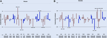
Studies using different model specifications analyzing different periods were unable to reject the null hypothesis that the residuals are random error (Bond and Fleisher Reference Bond and Fleisher1990, chap. 8; Cohen, Bond, and Fleisher Reference Cohen, Bond and Fleisher2013; Fleisher and Bond Reference Fleisher and Bond1983, Reference Fleisher and Bond1992; Fleisher, Bond, and Wood Reference Fleisher, Bond, Dan Wood, Rockman and Waterman2008). Even the tried-and-flawed “inter-ocular test”—eyeball the plot, and if a pattern hits you between the eyes, it’s significant—failed to reveal expected patterns. An updated analysis of annual presidential success rates from 1953–2014 explains 89% of the variance in the House and 72% in the Senate with three variables (party control, public approval, and party polarization) plus interactions. Footnote 5 Figure 1 plots studentized residuals from these regressions. Footnote 6 Diagnostics found no evidence of heteroscedasticity, autocorrelation, specification error, or omitted variables. Moreover, the “inter-ocular test” again failed to find evidence that Johnson and Reagan won significantly more than should be expected, or that Nixon and Carter won less. Perhaps sabermetrics can provide additional leverage on estimating presidents’ wins above expectations.
Regression Estimates of Presidents’ Wins Above Expectation in Congress

SABERMETRIC ESTIMATES OF PRESIDENTIAL WINS ABOVE EXPECTATIONS
Political scientists chase the god of statistical significance (anything more likely than .05 must be rejected) in search of theory. Sabermetricians chase the god of big (really big) data in search of accurate predictions. With big data, statistical significance and theory fade into irrelevance as ever more accurate of predictions reveal empirical truth. If asked about theory, a sabermetrician might reference Alfonso Bedoya in Treasure of the Sierra Madre: “Theory? We ain’t got no theory. We don’t need no . . . stinkin’ theory!” Footnote 7 So let’s take off our shoes and sox and see what shoeless empiricism reveals.
Pythagorean Expectations
Bill James’ (Reference James1982) Pythagorean Expectations formula is perhaps the foundational element of sabermetrics. It predicts Major League Baseball teams’ winning percentages with over 90% accuracy based solely on runs scored and runs allowed:
 $$Win\,Percentage = {{runs\,score{d^\gamma }} \over {runs\,score{d^\gamma } + runs\,allowe{d^\gamma }}}$$
The central insight of James’ PE formula is that runs scored and runs allowed reveal information about a team’s performance beyond whether it won or lost any particular game. Although the binary outcome may be the primary concern—Does the team win the game? Does the president win the roll call?—binary outcomes are the product of some continuous underlying data generating process. Each run scored or allowed implies a story of successes or failures that culminated in a win or loss, and so runs scored and runs allowed are better indicators of actual team performance—Are the hitters scoring? Are the pitchers and fielders making outs?—than is simple winning percentage. Over the course of a 162 game season for 30 Major League franchises, winning percentage and PE converge quite closely. In James’ original formulation, the value of γ was set at 2 for the sake of simplicity and because it fit the data reasonably well. Footnote 8 Since then, the PE formula for major league baseball has been refined to arrive at γ =1.82 as the exponent that generates the most accurate predictions (Miller Reference Miller2007).
PE does not perfectly predict actual winning percentages, and sabermetricians hotly debate the meaning of deviations from PE, or Wins Above Expectations (WAE). Put simply, WAE is a measure of games that a team won that it should have lost (positive WAE), or lost that it should have won (negative WAE), over the course of a season. For many, WAE is merely noise that reflects the irreducible randomness of a game played by humans under varying conditions. For others, WAE indicates the quality of relief pitching, the ability to hit or pitch “in the clutch” (i.e., in high-leverage situations), or—critically for our purposes—the skill of a team’s manager. Footnote 9
WAE as a Measure of Managerial Skill
The intuition behind WAE as a measure of managerial skill is that, over the course of a season, a baseball team’s PE is mostly a function of the talent on its roster. A team full of elite athletes in their primes should score plenty of runs and allow few, with or without a great manager. Just so, a team with slower, weaker, or injury-prone players probably will score few runs and allow many, regardless of what its manager does. WAE, then, is argued to measure how effectively a manager deploys the talent at his disposal in close games.
Two championship seasons from the career of Hall of Fame manager Sparky Anderson—the 1976 Cincinnati Reds and 1984 Detroit Tigers—are instructive. Fresh off a World Series championship in 1975, the 1976 Reds were a juggernaut—the team’s roster boasted three future Hall of Famers (plus Pete Rose, whose off-field transgressions have kept him from enshrinement). Dubbed the “Big Red Machine” in the press, the team cruised to a 102–60 record, ten games ahead of the second-place Dodgers, and swept the playoffs en route to a second consecutive World Series title. Although baseball fans revere the 1976 Reds as one of baseball’s all-time greatest teams, its 102 wins were actually less than its Pythagorean Expectation of 103–59, giving Sparky Anderson a -1.0 WAE (or -0.62 WAE%) for the season.
By contrast, the 1984 Tigers were building on a solid but unspectacular performance in 1983 with a roster that included no Hall of Famers. Footnote 10 Yet the 1984 Tigers led the American League all season, swept the Royals to win the American League pennant, and beat the Padres in five games to win the World Series. The 1984 Tigers’ 104–58 record exceeded their Pythagorean Expectation by five games, giving Anderson an extraordinary 5.0 WAE and 3.09 WAE%. Not coincidentally, Anderson was named the 1984 American League Manager of the Year.
The point of the illustration is simple but enlightening. The 1976 Reds were expected to crush the National League with their talent-laden roster, so the team’s excellent record and championship offer little evidence of Anderson’s managerial prowess; the 1984 Tigers were expected to be merely good, so the team’s dominant performance that year suggests that Anderson’s management contributed to its success.
Presidential PE in Congress
Can the PE formula be adapted to predict presidential success in Congress? We observe a number of parallels between presidential-congressional relations and baseball. The president is analogous to a manager. A roll call is analogous to a game that the president’s team plays. Votes supporting and opposing the president are analogous to runs scored and allowed in each “game.” A year is analogous to a season. A president whose party holds large majorities in both houses of Congress is akin to a manager with an all-star roster; we would expect such a president to win most roll calls without extraordinary effort. A president who faces hostile majorities in Congress is like the manager of a team full of poor hitters and soft-tossing pitchers who struggle to throw strikes; under such conditions, any roll call wins at all might be evidence of the president’s political skill, even though the actual winning percentage is low.
We observe a number of parallels between presidential-congressional relations and baseball. The president is analogous to a manager. A roll call is analogous to a game that the president’s team plays. Votes supporting and opposing the president are analogous to runs scored and allowed in each “game.” A year is analogous to a season. A president whose party holds large majorities in both houses of Congress is akin to a manager with an all-star roster; we would expect such a president to win most roll calls without extraordinary effort.
Just as James’ PE formula recognized that runs scored and allowed convey information about team performance that is not reflected in winning percentage, votes won and lost on presidential roll calls may contain information about presidential performance beyond an annual winning percentage. Each vote for or against the president carries information about legislative politics, including party control, party cohesion, and public approval. The typical regression analysis considers each of these variables separately on the right-hand side of its equation with specific causal theories in mind. The PE approach is unapologetically atheoretical, aggregating votes over a year as a way of approximating the overall strength of a president’s legislative sway apart from any one roll call, just as the baseball PE measures the strength of a team’s roster apart from any one game. Adapted to presidential-congressional politics, the formula for Pythagorean Expected roll call winning percentage (PE%) is:
 $$PE\% = {{votes\,fo{r^\gamma }} \over {votes\,fo{r^\gamma } + votes\,agains{t^\gamma }}}$$
The difference between actual winning percentage and PE% is percentage Wins Above Expectations (WAE%). At the end of a year, a positive value indicates that the president won more roll calls than expected, while a negative value indicates more losses than expected. This percentage multiplied by the number of roll calls on which the president took a position yields Wins Above Expectations (WAE). Just as some baseball analysts use WAE to assess managerial skill, WAE might also yield information about presidents’ skill with legislative politics. As with baseball managers, WAE% offers a useful way to think about presidents’ annual performance, while total WAE rewards performance across several years and so offers some perspective on career legislative accomplishments.
The need to use WAE% rather than WAE highlights two important differences between baseball games and congressional roll calls. Footnote 11 First, whether enjoying a winning season or suffering through a miserable one, every Major League team plays 162 games. “You win a few, you lose a few, some get rained out,” Satchel Paige once observed, “but you got to dress for all of them.” Presidents win a few and lose a few, but unlike ballplayers, presidents don’t have to dress for all of them. Instead, presidents get to pick which “games” to play when they choose whether to take a position on a particular roll call. Being able to pick their votes raises the possibility that a president may seek to manipulate their success rate and WAE by sitting out a sure loser or stepping up to endorse a sure winner. Although a president may occasionally engage in such posturing, Peterson (Reference Peterson1990) presents evidence that presidential positions are generally sincere. And Covington (Reference Covington1987b) finds evidence that the president can occasionally increase the chances that a roll call will go their way by “staying private.” Such cases are rare, but these “wins” do not appear in the success rate because the president remained in the clubhouse. Nevertheless, analysis of presidential “dressing for the game” reveals no evidence that presidents’ position taking systematically affects their actual legislative success rate or WAE (see appendix A).
Second, for analytical purposes, in baseball each run scored is an independent event: the probability that a team will score or allow a run in a given game is essentially unrelated to the runs scored and allowed in the previous and subsequent games. One reason for the success of sabermetrics is that baseball scoring satisfies the independent, identically distributed (IID) assumption. The validity of the IID assumption for congressional roll calls is more questionable: the probability that a president will lobby effectively on legislation may depend on their past success or future legislative agenda. In this analysis, however, such a violation of the IID assumption might be analytically useful if the interdependence of roll calls reveals something about Neustadt’s Political Skills hypothesis. Presidents may gain or lose momentum during a given session of Congress as a function of their legislative skill. With this caveat in mind, we now apply a sabermetric framework to presidential politics.
Calculating Presidential PE
Following standard sabermetric procedures, we used the presidential roll call vote data described earlier to calculate PE WAE% and WAE for presidents. Votes for and against the president’s position were totaled for roll calls on which the president took a position for each year from 1953–2014 (n=4231 House votes, 4356 Senate votes). Footnote 12 Using these totals, we calculated PE for each year with γ set to 2 using James’ (Reference James1982) original formulation. The result was a striking .934 Pearson correlation between PE% and actual winning percentage in the House and .907 in the Senate. These impressive correlations belied substantial year-to-year error, so we followed the usual sabermetric practice of minimizing squared differences between PE% and actual winning percentage. We applied a Generalized Reduced Gradient (GRG) iterative algorithm to the PE% formula and roll call voting data with an aim of minimizing squared differences, with γ constrained to be greater than zero and less than 100. The GRG algorithm is an efficient, robust method for optimizing nonlinear problems (Mantell and Lasdon Reference Mantell and Lasdon1978). Footnote 13 Optimization yields γ values of 3.44 in the House and 3.11 in the Senate. Thus, the PE% formulae for presidents are:
 $$House\,PE\% = {{votes\,fo{r^{3.44}}} \over {votes\,fo{r^{3.44}} + votes\,agains{t^{3.44}}}}\,\,Senate\,PE\% = {{votes\,fo{r^{3.11}}} \over {votes\,fo{r^{3.11}} + votes\,agains{t^{3.11}}}}$$
RESULTS OF SABERMETRIC ANALYSIS OF PRESIDENTIAL WINS ABOVE EXPECTATIONS
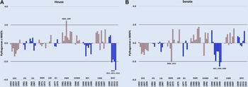
These formulas generate PE% that correlate .939 with actual winning percentages in the House and .829 in the Senate. Footnote 14 The slightly higher γ value for the House reflects the wider average winning margins in that chamber. Footnote 15 Figure 2 shows annual WAE% for House and Senate, standardized to facilitate comparison to the studentized residuals from the regression analysis.
Pythagorean Presidential Wins Above Expectations

Although the regression models and the PE formula predict presidential success rates with similarly high levels of accuracy, the WAE% from the two approaches are uncorrelated (r2 = 0.001 and House and 0.078 in the Senate). The patterns of PE WAE% are quite different from those estimated by studentized residuals. The studentized residuals indicate that each president exceeded expectations in some years and fell short in others more or less at random in both chambers—exactly as expected for regression models. The PE estimates, however, indicate that presidents generally were consistently above or below expectations in both chambers across the years of their administrations. In particular, Reagan was considerably above the mean in both the House and Senate during all eight years. Clinton was below the mean for all but one or two years of his presidency, and well below in the Senate. Obama exceeded expectations in the House during his first two years, but falls far below the mean in the next four years.
Moreover, the PE approach produces a strong partisan pattern: Republican presidents outperform Democrats. Ike is in last place, but otherwise the top WAEs are all GOP. Neither regression analysis nor case studies and scholar surveys find evidence of a party advantage.
Sabermetric Analysis of Neustadt’s Skills Hypothesis
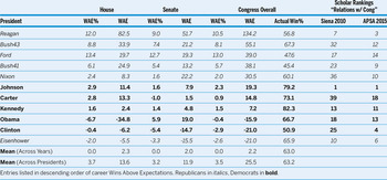
How does Neustadt’s Political Skills Hypothesis fare with sabermetric WAE? Do presidents who are renowned for legislative skill generate impressive WAE? And does WAE% in the House correlate with WAE% in the Senate, as the skills hypothesis suggests? To address these questions, we used PE% to calculate annual WAE% and WAE for each chamber. We also calculated each president’s “career average” WAE% and WAE by summing their annual WAE across chambers. Table 1 reports these results Footnote 16 ordered by career WAE. Footnote 17
Sabermetric Wins Above Expectations

Sabermetric analysis offers mixed support about the political skill of the reputed legislative giants Lyndon Johnson and Ronald Reagan. Johnson’ career statistics place him first among Democrats, but in the middle of the lineup overall, with House (hWAE% = 2.9, hWAE=11.4) and Senate (sWAE%=1.6, sWAE=7.9) averages below the mean among post-WWII presidents. In contrast, Reagan’s career statistics make him by far the most impressive legislative operator in the sample, ranking second in career WAE% and an easy first place in WAE in both houses. Reagan’s career hWAE of 82.5 and sWAE of 51.7 are more than double his next closest rival’s.
On the low end of the reputational distribution are Richard Nixon and Jimmy Carter. Here, sabermetric assessment diverges from the scholarly consensus. Their WAEs are near the middle of lineup—Nixon ranks #5 (just ahead of LBJ), with Carter just behind him. In sabermetric terms, it is more accurate to describe their legislative records as “mediocre” rather than “bad.”
Finally, Neustadt does not suggest that influencing the House and Senate requires different skills, so we should observe similar patterns in both chambers. Sabermetrics offer some support for this expectation. The Spearman rank-order correlation of career House and Senate WAE% is .69 (p=.02), indicating that the rankings are broadly similar in both chambers.
Sabermetric Analysis vs. Scholars’ Reputational Rankings
For comparison to a non-quantitative assessment, table 1 also reports each president’s ranking on their “Relations with Congress” from the 2010 Siena Presidential Expert Poll of presidential scholars, and a 2015 poll of political scientists who are members of the Presidency and Executive Politics Section of APSA (Rottinghaus and Vaughn Reference Rottinghaus and Vaughn2015).
Both polls rank Johnson the top legislative leader and Carter last, but there is less consensus about the rankings in between (Spearman’s ρ=.591, p=.06). The ranking based on sabermetric career WAE, however, is uncorrelated with either poll (ρ=-.009 with the Siena poll and ρ=-.036 with the APSA poll). The lack of correlation implies that presidential experts apply their own adjustments to presidents’ legislative records to account for context, but evidently not the same kinds of adjustments as those implied by PE. As with sabermetricians and traditional sports writers, quantitative analytics and expert qualitative assessments lead to different conclusions about presidents’ legislative prowess.
How do we reconcile these differences between presidents’ historic reputations and their sabermetric profiles? Baseball again offers an enlightening metaphor: in sabermetric terms, the managerial careers of Joe Torre and Bobby Cox parallel the legislative records of presidents Johnson and Reagan. Torre and Cox each managed major league teams over 29 years, both are widely considered all-time great managers, and both were inducted to the Hall of Fame in 2014. Over his managerial career, Torre won 2,326 games (.538 winning percentage), six American League pennants, and four World Series titles; Cox won 2,504 games (.556 winning percentage), five National League pennants, and one World Series. But their places on Darowski’s all-time managers’ WAE list are quite different: Footnote 18 Cox ranks 4th with a career WAE of 77.0, but Torre’s respectable 23.3 WAE puts him far behind at 39th. A close look at their records makes the reason clear: Torre’s most successful years came with the New York Yankees between 1996 and 2007, when his roster included some of the most fearsome players in baseball. Torre’s Yankees teams won big, but they were supposed to win big based on their enormous payrolls and all-star laden rosters. Cox spent nearly his entire managerial career with the talented but less-than-awesome Atlanta Braves, winning consistently and routinely outperforming his PE.
Like Torre and Cox, Johnson and Reagan earned their reputations in different ways. Johnson’s actual legislative winning percentages are high, but not much better than his high PE. Johnson won most of his legislative battles, including some extraordinary legislative “championships” with civil rights laws and Medicare. But like Torre’s Yankees of the late-1990s and early-2000s, LBJ was expected to win with his strong partisan majorities in both houses and a booming economy. Reagan’s actual winning percentages are relatively low (.420 House, .720 Senate), but like Bobby Cox, his record was consistently much higher than his PE, particularly in the House. Torre, Cox, Johnson and Reagan were all successful and probably deserving of their places in their respective Halls of Fame. But sabermetrics makes a stronger case for Cox and Reagan, while traditionalists would point to Torre’s four World Series rings and Johnson’s landmark legislative achievements in making their arguments for enshrinement.
DISCUSSION
This analysis shows that the Pythagorean Expectations formula predicts presidential success rates about as accurately as well-specified regression models. What PE extracts from the sum of votes supporting and opposing the president, however, is different from the theoretical explanations of presidential success—the interaction of party control, public approval, and party polarization—included in our regression models. But unlike regression residuals, presidential WAE suggests that some presidents have been consistently above or below expectations. Presidential WAE also diverges markedly from scholars’ collective, qualitative judgment of presidents’ legislative efficacy as measured by widely cited surveys. Perhaps WAE is capturing something about crafting legislative coalitions, but as is the case with regression residuals and expert judgments, we don’t know exactly what underlies the data generating process.
Sabermetrics may be a useful tool to analyze presidential success on roll call votes, but this paper barely scratches the surface. The more important contributions of sabermetrics to baseball are estimating players’ Wins Above Replacement (WAR) to show how much each one contributes to his team’s success. The parallel between members of the president’s party and players, however, is much less clear than the parallel between votes and runs. At the very least, we think sabermetrics may offer a new, WAE cool direction for the study of presidents’ participation in legislative politics.
SUPPLEMENTARY MATERIAL
To view supplementary material for this article, please visit https://doi.org/10.1017/S1049096516002778
ACKNOWLEDGMENTS
We are grateful to Carlisle Rainey, Guy Whitten and the participants in the Program in Scientific Political Methodology at Texas A&M University for helpful comments and suggestions.