



1 Introduction
The flow produced by the motion of a bluff body in a fluid is ubiquitous in industrial applications. One of the cases frequently encountered concerns the transport industry, especially for ground vehicles such as cars or lorries. The bluffness associated with a functional blunt geometry is responsible for a massive flow separation at the rear leading to complex wake dynamics and large pressure drag. The growing constraints on energy saving have led to a thorough study of these flows in order to fundamentally understand the mechanisms of drag generation and develop efficient flow control methodologies.
Symmetry breaking in the wake of a bluff bodies and its relation to drag. (a) Bifurcation scenario of the wake of a sphere in the laminar regime adapted from Pier (Reference Pier2008). Drag of the sphere depending on the flow regime: steady axisymmetric, SA (thick black line); steady planar symmetric, SPS (dashed line); and unsteady planar symmetric, UPS (thin blue lines delimiting maxima and minima) (see respectively figures 1, 4 and 3 of Pier (Reference Pier2008) for the wake flow associated with each regime). (b) Bifurcation scenario of the wake of an Ahmed body in the laminar regime adapted with permission from Grandemange, Gohlke & Cadot (Reference Grandemange, Gohlke and Cadot2012) (copyright of the American Physical Society). Back-view flow visualization of the wake in the steady symmetric state at a  $Re=310$ (based on the height of the body) and the steady asymmetric state at
 $Re=365$.

The structure of the recirculating flow in the near wake surrounded by developing shear layers leads to a rich set of dynamics involving very different spatial and time scales. One of the main peculiar features of these wake flows is the symmetry-breaking instability leading to a high degree of asymmetry in the wake despite the symmetry properties of the geometry. The case of the sphere is a particularly illuminating example as the theoretical studies of Bouchet, Mebarek & Dušek (Reference Bouchet, Mebarek and Dušek2006) and Pier (Reference Pier2008) have been the only ones to provide an objective quantification of the influence of loss of flow symmetry on the drag. At diameter-based Reynolds number  $Re\sim 210$ the axisymmetry of the wake SA is lost and the flow selects a single plane of symmetry (SPS). An important consequence of this loss of axisymmetry is the additional drag generated by the SPS wake. The evolution of the drag coefficient of the sphere
 $C_{D}$ with
 $Re$ of the different stable and unstable flow configurations from Pier (Reference Pier2008) is reproduced in figure 1(a). Around 6 % to 7 % of the total drag of the sphere is ascribed to the loss of axisymmetry in favour of planar symmetry. Very similar symmetry-breaking scenarios can be drawn for the case of the normal disk (Natarajan & Acrivos Reference Natarajan and Acrivos1993; Meliga, Chomaz & Sipp Reference Meliga, Chomaz and Sipp2009) or the bullet-shaped body (Sevilla & Martínez-Bazán Reference Sevilla and Martínez-Bazán2004; Bohorquez et al. Reference Bohorquez, Sanmiguel-Rojas, Sevilla, Jiménez-González and Martínez-Bazán2011), which generalizes the behaviour of the wake flow past axisymmetric bluff bodies. Interestingly, when further increasing
 $Re$ to the turbulent regime, the axisymmetry of the sphere and the bullet-shaped body are restored in a statistical sense according to recent experiments by Grandemange, Gohlke & Cadot (Reference Grandemange, Gohlke and Cadot2014a) and Rigas et al. (Reference Rigas, Oxlade, Morgans and Morrison2014) performed respectively for the sphere at
 $Re=2\times 10^{4}$ and the bullet-shaped body at
 $Re=2\times 10^{5}$. Actually, at these high
 $Re$, the large-scale organization of the wake is still planar symmetric but only in the instantaneous sense. This plane of symmetry rotates randomly over very long time scales of order 100 to 1000 convective time units, and the azimuthal orientation of the plane
 $\unicode[STIX]{x1D703}_{W}$ explores equiprobably all possible orientations. However, once the axisymmetry of the geometry is perturbed, as in the study of Grandemange et al. (Reference Grandemange, Gohlke and Cadot2014a) (or the study of Gentile et al. (Reference Gentile, Van Oudheusden, Schrijer and Scarano2017) for the bullet-shaped body) which mimics the presence of side holding wires on the sphere, the statistical axisymmetry is broken and the instantaneous plane of symmetry explores preferentially azimuthal positions
 $\unicode[STIX]{x1D703}_{W}$ the most distant from the perturbations positions (i.e.
 $\unicode[STIX]{x03C0}$ for a
 $m=1$ perturbation at
 $\unicode[STIX]{x1D703}_{W}=0$ or
 $\pm \unicode[STIX]{x03C0}/2$ for a
 $m=2$ perturbation at
 $\unicode[STIX]{x1D703}_{W}=0$ and
 $\unicode[STIX]{x03C0}$).
When the number of symmetry planes of the geometry is finite, as in the case of rectangular cross-sectioned blunt bodies like the Ahmed body (Ahmed, Ramn & Faltin Reference Ahmed, Ramn and Faltin1984), wake dynamics is in the continuity of the axisymmetric case and its perturbed dynamics. Grandemange et al. (Reference Grandemange, Gohlke and Cadot2012) and Evstafyeva, Morgans & Dalla Longa (Reference Evstafyeva, Morgans and Dalla Longa2017) showed, respectively, experimentally and numerically how the laminar flow past an Ahmed body follows a first bifurcation breaking the last plane of symmetry of the model in ground proximity and deviating the wake permanently on one side as shown in figure 1(b). Grandemange et al. (Reference Grandemange, Mary, Gohlke and Cadot2013c) showed how the turbulent regime restores the planar symmetry of the set-up in a statistical sense but with an instantaneous asymmetry. The instantaneous asymmetry of the wake manifests as a lateral asymmetry and random side reversals of the wake to statistically restore the symmetry. This bi-stable behaviour is characterized by a Poissonian random flipping motion of the wake from one side to the other with a characteristic residence time of  $10^{3}$ convective time units in an asymmetric state. The aspect ratio between height and width of the base
 $H/W$ and the ground clearance
 $G$ have a strong influence in determining the direction of the symmetry-breaking instability in the turbulent regime. Grandemange, Gohlke & Cadot (Reference Grandemange, Gohlke and Cadot2013a) have drawn a landscape of this bi-stable feature of the wake in the parameter plane
 $(H/W,G)$ which was also numerically assessed by Dalla Longa, Evstafyeva & Morgans (Reference Dalla Longa, Evstafyeva and Morgans2019) for the original Ahmed body and its inverted stream-normal aspect ratio version. Nevertheless, this symmetry-breaking dynamics in the wake of the Ahmed body appears to be highly sensitive to small flow perturbations. Barros et al. (Reference Barros, Borée, Cadot, Spohn and Noack2017) showed how small geometric perturbations in the underbody (typically cylinders of diameter one to two order of magnitude smaller than
 $H$) strongly affect the asymmetry direction of the wake. The study drew a complete bifurcation scenario suggesting a competition between vertical and lateral asymmetries with an evolution from purely lateral bi-stable asymmetries to purely vertical static asymmetries depending on the size of the perturbation. Bonnavion & Cadot (Reference Bonnavion and Cadot2018) further formalized this sensitivity study by looking at the influence of small changes on the wake asymmetries of the pitch angle of the Ahmed body, the yaw angle (as done by Cadot, Evrard & Pastur (Reference Cadot, Evrard and Pastur2015) also), the ground clearance or the stream-normal aspect ratio of the body. The work provides a description of the symmetry-breaking instability as an analogue to the axisymmetric case of the sphere and the bullet-shaped body discussed previously with two specific modifications: an elliptic modulation of the degree of asymmetry due to the aspect ratio
 $H/W$ of the body, and an alignment of the admissible asymmetry orientations on the two planes of symmetry of the geometry, which echoes the sensitivity study of the sphere wake from Grandemange et al. (Reference Grandemange, Gohlke and Cadot2014a).
Barros et al. (Reference Barros, Borée, Noack, Spohn and Ruiz2016), Li et al. (Reference Li, Barros, Borée, Cadot, Noack and Cordier2016) and Li et al. (Reference Li, Borée, Noack, Cordier and Harambat2019) showed how low frequency forcing on one side of the base targeting time scales comparable to the dominant ones of the shear layer has authority to flip the asymmetry of the Ahmed body wake. Low frequency flow control strategy were used in order to mitigate the lateral bi-stable dynamics in the wake of the Ahmed body. Li et al. (Reference Li, Barros, Borée, Cadot, Noack and Cordier2016) used a simple closed-loop opposition control scheme with pulsed jets on both sides of the base in order to force the wake on either side depending on the lateral position of the wake. A mean symmetrization was achieved with a wake meandering around the completely symmetric state. However, it came only with an associated 2 % pressure drag decrease due to the increased turbulent activity in the shear layers caused by the forcing. Moreover, the side-alternating control promotes the vortex shedding dynamics in the wake resulting in a detrimental impact on the drag. Similarly, Brackston et al. (Reference Brackston, de la Cruz, Wynn, Rigas and Morrison2016) with oscillating side flaps and Plumejeau et al. (Reference Plumejeau, Delprat, Keirsbulck, Lippert and Abassi2019) also with pulsed jets have shown similar mixed 2 % drag reduction using similar feedback control with linear control methods. To mitigate the lateral bi-stable dynamics, only passive control methods have proven to be satisfyingly efficient in terms of associated drag reductions. Grandemange et al. (Reference Grandemange, Gohlke and Cadot2014a) mitigated the instability using a small vertical control cylinder localized in the middle of the wake with an associated base pressure recovery of approximately 5 %. The studies of Evrard et al. (Reference Evrard, Cadot, Herbert, Ricot, Vigneron and Délery2016) and Lucas et al. (Reference Lucas, Cadot, Herbert, Parpais and Délery2017) (also confirmed by Bonnavion (Reference Bonnavion2018)) have shown how a cavity placed at the base of the Ahmed body could completely eliminate the symmetry breaking, leading to lateral bi-stability provided that the cavity is long enough (approximately  $0.3H$). Nevertheless, both control techniques are quite invasive in terms of geometrical modifications, and even unpractical to arrange on a real configuration for the control cylinder.
Even if all these recent works give important insight into the behaviour of the symmetry-breaking instability in three-dimensional blunt body wakes, there still remains an important open question concerning the mechanism of symmetry breaking and its relation to drag generation. The objective of this paper is thus to further elucidate the mechanics of drag reduction observed during transient near-wake reversals and the increase of drag in asymmetric states. In particular, we will show how transient symmetric states of the near wake explored during the reversals differ from the static symmetry-breaking states. This will be addressed by studying the coupling between lateral shear layers showing very distinct unsteady structures in static or transient states. The paper is organized as follows. The experiments are first described in § 2. A global sensitivity study of the wake asymmetry and its relation to base drag is provided in § 3. Then transient near-wake reversals are characterized using conditional and ensemble-averaged descriptions in § 4. The peculiar coupled dynamics between the recirculating flow and the shear layers is characterized in § 5 to provide a link between asymmetries and drag. This leads in § 6 to the characterization of the flow dynamics during the transient wake reversals. Finally, based on the results, a thorough discussion of the asymmetric flow dynamics, its relation to the drag and its control is proposed in § 7.
Experimental set-up. (a) Arrangement of the model inside the test section. (b) Pressure tap location on the base: points indicate mean pressure measurements location and circles time-resolved pressure measurements. Both measurements are used for different purposes (see text for details). (c) Disposition of the spanwise cylinders of diameter  $d$ used to passively perturb the natural equilibrium of the wake. (d) Time-resolved particle image velocimetry (PIV) field of view (FOV) in the horizontal plane
 $z=0.67H$ and definition of the yaw angle. (e) Method to trigger a lateral wake reversal. The model is yawed at an angle sufficient to completely lock one of the lateral asymmetric states. Forcing at
 $St_{W}\sim 1$ on the windward side then maintains the wake in the opposite asymmetric state. When the forcing is stopped, the wake relaxes to the initial lateral asymmetric state producing a wake reversal. The whole process is captured by the time-resolved measurements.

2 Description of the experiments
This section describes the set-up of the bluff body in the wind tunnel and the different measurement techniques used. In addition, we expose details on the techniques used to perturb the wake and investigate the near-wake reversals.
2.1 Wind-tunnel facility and model geometry
The experiments are performed inside the working section of a subsonic wind tunnel of  $2.4~\text{m}$ width and
 $2.6~\text{m}$ height. The turbulence intensity of the upstream flow is of the order of 0.3 % at most operating conditions with flow homogeneity better than 0.5 %. A sketch of the bluff body arrangement inside the working section is given in figure 2(a). The front of the model consists in curved edges rounded with a non-constant radius leading to a smooth curvature transition with the flat side surfaces of the model. This is aimed at minimizing the flow detachment just after the rounded front surface, limiting its impact on the downstream wake flow (Spohn & Gilliéron Reference Spohn and Gilliéron2002). The model with height
 $H=0.3~\text{m}$, width
 $W=0.36~\text{m}$ and length
 $L=1~\text{m}$ (with an aspect ratio
 $H/W=0.83$ slightly higher than the original geometry of Ahmed et al. (Reference Ahmed, Ramn and Faltin1984)) is fixed on a raised false floor with a ground clearance
 $G=0.05~\text{m}$ which corresponds to approximately five times the thickness of the turbulent boundary layer upstream of the model. The influence of flow blockage above the raised floor was neglected due to a low blockage ratio of 2.2 %. An inclinable flap fixed at an upwards angle of
 $\unicode[STIX]{x1D6FC}=1^{\circ }$ ends the raised floor in order to compensate for the lift and the streamwise pressure gradient generated by the whole set-up.
All the experiments carried out in this work are performed at  $U_{0}=25$ m s
 $^{-1}$ or
 $Re_{H}=U_{0}H/\unicode[STIX]{x1D708}=5\times 10^{5}$ where
 $\unicode[STIX]{x1D708}$ is the kinematic viscosity of the air at operating temperature. The boundary layer at separation at the rear edges of the model is fully turbulent with a characteristic momentum thickness
 $\unicode[STIX]{x1D703}_{0}=2.2\times 10^{-3}$ m measured by hot-wire anemometry. We use conventional notations in the Cartesian coordinate system with
 $x$,
 $y$ and
 $z$ for respectively the streamwise, spanwise and cross-stream or transverse directions (accordingly
 $\boldsymbol{u}=(u_{x},u_{y},u_{z})$ for the velocity field) with the origin
 $O$ arbitrarily located on the floor in the vertical plane of symmetry of the model. Unless otherwise specified, all physical quantities are normalized by any appropriate combination of the physical parameters
 $H$,
 $U_{0}$ and
 $\unicode[STIX]{x1D70C}$, the air density at operating conditions. In the remainder of the paper, the Reynolds decomposition of a quantity
 $\unicode[STIX]{x1D712}$ in its time-averaged
 $\overline{\unicode[STIX]{x1D712}}$ and fluctuating
 $\unicode[STIX]{x1D712}^{\prime }$ parts is introduced such as
 $\unicode[STIX]{x1D712}=\overline{\unicode[STIX]{x1D712}}+\unicode[STIX]{x1D712}^{\prime }$.
2.2 Pressure measurements
To perform surface pressure measurements on the model, two different systems have been used. First, a 64-channel ESP-DTC pressure scanner linked to 1 mm diameter pressure tappings around the model (35 taps on the base, see figure 2b) by  $80~\text{cm}$ long vinyl tubbing was used for static pressure measurements sampled at
 $200~\text{Hz}$ with a range of
 $\pm 1~\text{kPa}$. In addition, 12 differential pressure sensors SensorTechnics HCLA 02X5DB, the distribution of which is given in figure 2(b), are used with a reduced
 $25~\text{cm}$ tubbing length and proper frequency response calibration for time-resolved measurements with a bandwidth of
 $2~\text{kHz}$ (Ruiz et al. Reference Ruiz, Sicot, Brizzi, Laumonier, Borée and Gervais2009). These operate in a range of
 $\pm 250~\text{Pa}$ and acquisition is performed at twice the cutoff frequency, hence
 $4~\text{kHz}$. Measurement incertitude of both systems lies respectively below
 $\pm 1.5$ Pa and
 $\pm 0.7$ Pa, which represents less than
 $2\,\%$ of the mean base pressure. Pressure measurements are expressed in terms of the pressure coefficient
 $C_{p}$ defined as
 $$\begin{eqnarray}C_{p}=\frac{p-p_{0}}{0.5\unicode[STIX]{x1D70C}U_{0}^{2}}.\end{eqnarray}$$
The reference pressure  $p_{0}$ is taken at
 $x/H=-2$ above the model by a Pitot tube mounted at the ceiling of the test section. For global results presented in § 3, pressure measurements are performed over 12 to 15 min, which corresponds to
 $5$ to
 $7.5\times 10^{4}$ convective time units
 $H/U_{0}$ and is sufficient for statistical convergence of the measurements.
2.3 Aerodynamic force measurements
To quantify the total drag, the model was directly mounted on a 6-component aerodynamic balance (9129AA Kistler piezoelectric sensors and 5080A charge amplifier). The balance has been in-house calibrated using known masses and a system of pulley applying pure forces, pure moments or a combination of both on the balance. A whole volume including the expected application point of the aerodynamics tensor of the model has been covered for calibration by using various level arm length for moments. Total measurement incertitude is less than 0.6 % of the full scale range, which represents less than 1 % incertitude on the mean drag force  $F_{x}$ for instance. Drag measurements are expressed as a non-dimensional drag coefficient
 $$\begin{eqnarray}C_{x}=\frac{F_{x}}{0.5\unicode[STIX]{x1D70C}U_{0}^{2}HW}.\end{eqnarray}$$
Measurements were performed simultaneously with the pressure measurements, leading to similar conclusions concerning their statistical convergence.
2.4 Velocity measurements
Particle image velocimetry is performed in the near wake of the model to gain insight into the flow structure. The set-up is associated with a large FOV spanning the whole recirculating wake (approximately  $1.8H$ (length)
 $\times 1.3H$ (width)) in the horizontal plane of symmetry of the model (plane
 $z/H=0.67$) as shown in figure 2(d). Time-resolved PIV (TR-PIV) is deployed to investigate the transient dynamics of lateral wake reversal. A Phantom VEO4K 990 camera (sensor of
 $4096\times 2300~\text{px}$) coupled to a Sigma DG Macro 105 mm objective is used to image this FOV in a double-frame mode at a frequency of 500 Hz. In order to have sufficient illumination of the PIV plane, two lasers Continuum Terra PIV
 $2\times 30~\text{mJ}$ and Quantronix Darwin Duo
 $18~\text{mJ}$ are synchronously fired from each side of the test section. The flow is seeded from downstream the raised floor by atomization of mineral oil producing
 $1~\unicode[STIX]{x03BC}\text{m}$-diameter particles. Multi-pass cross-correlation is performed using Davis 10.1 with a final interrogation window of
 $12\times 12$ pixels and overlap of 50 %. For this set-up, care is taken to resolve both temporally and spatially the most important scales in the wake. The frame rate is sufficient to resolve the smallest time scales associated with the initial shear-layer instability after separation of the turbulent boundary layer. This time scale is estimated to be
 $T_{\unicode[STIX]{x1D703}}=St_{\unicode[STIX]{x1D703}_{0}}U_{0}/\unicode[STIX]{x1D703}_{0}\sim 230~\text{Hz}$ where
 $St_{\unicode[STIX]{x1D703}_{0}}\sim 0.022$ is the initial most amplified time scale in a turbulent shear layer according to Zaman & Hussain (Reference Zaman and Hussain1981). Similarly the spatial resolution of the velocity measurements is approximately
 $1~\text{mm}$, which is less than half of
 $\unicode[STIX]{x1D703}_{0}$. A total of 17 natural and triggered transient wake reversals each between 2000 and 2800 image pairs have been acquired using this set-up representing 4 to 5.6 s for each realization. All these characteristics are summed up in table 1. The maximum uncertainty on the velocity measurements based on a 0.1 px uncertainty is estimated to be less than
 $0.01U_{0}$.
PIV characteristics of the wake reversal experiments. The total duration and number of images only refer to the wake reversal period itself.

2.5 Passive perturbation of the wake equilibrium
The symmetry of the Ahmed body flow is passively perturbed in different ways. The yaw angle  $\unicode[STIX]{x1D6FD}$ can be changed in order to influence the lateral symmetry of the flow (figure 2d). Independently, the vertical symmetry of the flow is perturbed using spanwise cylinders of different diameters
 $d$ ranging from
 $0.01H$ to
 $0.066H$ placed either on top or below the body as sketched in figure 2(c). This range of
 $d$ represents from approximately 1 to
 $6\unicode[STIX]{x1D703}_{0}$. Two different locations upstream from the base have been tested, namely
 $x/H=-1$ or
 $-2$, without noticeable influence on the effect they have on the wake. The results presented herein correspond to the case
 $x/H=-2$ for brevity without loss of generality.
2.6 Capturing time-resolved wake reversals
An important aspect of this work is the detailed investigation of the wake reversals occurring in lateral asymmetric states of the wake. Fine investigations of the reversal process are studied using coupled TR-PIV and base pressure measurements as sketched in figure 2(b,d). The wake reversal is a Poissonian random process (Grandemange et al. Reference Grandemange, Gohlke and Cadot2013a). In order to only focus on the reversals and to acquire a sufficient number of them, two different strategies are adopted. As the TR-PIV can only record time segments of around 450 convective time units  $H/U_{0}$ and as the mean duration between two wake reversals is of order
 $O(1000H/U_{0})$, the capture of the wake reversal process is rather complex. The first method is to try to capture a wake reversal on the fly by hoping one occurs quite in the middle of the TR-PIV acquisition. This leads to important number of tries for only several wake reversal acquisitions. A second more efficient method is to trigger the reversals as sketched in figure 2(d). For this, the body is first yawed at an angle sufficient to lock permanently the wake in one of the lateral asymmetric states. Here this angle is chosen as
 $\unicode[STIX]{x1D6FD}=0.7^{\circ }$. which is slightly higher than the value needed to permanently lock the lateral asymmetry as shown in figure 5 without having an noticeable influence on the flow around the body itself. Then periodic forcing is applied on the windward side of the wake (
 $y<0$ for
 $\unicode[STIX]{x1D6FD}>0$) using pulsed jets (see Li et al. (Reference Li, Borée, Noack, Cordier and Harambat2019) for a description of a similar forcing, or Haffner (Reference Haffner2020) for a detailed description of the forcing apparatus) in order to lock the wake in the opposite asymmetric state following the results of Barros (Reference Barros2015) and Li et al. (Reference Li, Barros, Borée, Cadot, Noack and Cordier2016). Periodic forcing is issued at
 $St_{W}\sim 1$ at small amplitude with a maximal velocity of
 ${\sim}0.6U_{0}$ and a root-mean-square velocity of
 ${\sim}0.2U_{0}$. This frequency will be shown to be related to a peculiar dynamics of the shear layers in the wake. When forcing is stopped, the wake naturally relaxes to the initial lateral asymmetric state and the wake reversal is captured. With this method, wake reversals are more easily captured. In addition, as the wake is relaxed and not triggered by the forcing to realize the reversal, it results in a reversal with similar dynamics described in § 6 and base drag evolution described in § 4. The PIV characteristics for the wake reversals captured by each method are summarized in table 1. The typical wake reversal experiment captures approximately 5 s of flow during which a reversal of
 ${\sim}0.5$ s separates
 ${\sim}2$ s of flow in both lateral asymmetric states. An example of a wake reversal event is provided in the supplementary movie 1. In addition the flow locked only in asymmetric states has also been captured with the body yawed at
 $\unicode[STIX]{x1D6FD}=0.7^{\circ }$ as in the triggered wake reversal experiments.
3 Wake flow sensitivity: asymmetries and base drag
The focus is first put on the sensitivity of the wake asymmetries to perturbations to discuss their relation to the base drag of the Ahmed body. The asymmetry is characterized by the mean base pressure distributions in figure 3(a) and by the probability density function of the base centre of pressure (CoP) position  ${\mathcal{P}}(\,y_{b},z_{b})$ in figure 3(b). The coordinates
 $y_{b}$ and
 $z_{b}$ are defined as
 $$\begin{eqnarray}y_{b}=\frac{\mathop{\sum }_{i=1}^{N}y_{i}C_{p}(\,y_{i},z_{i},t)}{\mathop{\sum }_{i=1}^{N}C_{p}(\,y_{i},z_{i},t)},\quad z_{b}=\frac{\mathop{\sum }_{i=1}^{N}z_{i}C_{p}(\,y_{i},z_{i},t)}{\mathop{\sum }_{i=1}^{N}C_{p}(\,y_{i},z_{i},t)}\end{eqnarray}$$
over the  $N$ pressure taps at the base. In this section, to investigate the asymmetry/drag relation in a statistical sense, all configurations are investigated over 15 min experiments using the pressure scanner and signals are low-pass filtered at 10 Hz to focus on the slow dynamics of wake reversals.
Sensitivity of the wake to different vertically perturbed conditions. The arrows at bottom indicate where the perturbation is placed and points towards increasing diameter size  $d$. Natural unperturbed case,
 $d/H$
= 0.053 on top and
 $d/H=\{0.013,0.026,0.066\}$ on bottom. (a) Time-averaged base pressure coefficient distribution
 $\overline{C_{p}}$ on the base. (b) Probability density function (PDF) of the base pressure barycentre position
 ${\mathcal{P}}(\,y_{b},z_{b})$ normalized by its maximum value. Insets represent the conditional average of the different wake states for non-static asymmetries. Thin black dashed lines denote the
 $y_{b}=0$ and
 $z_{b}=0$ axes. (c) The PDF of the lateral base CoP position and the space-averaged base pressure coefficient
 ${\mathcal{P}}(\,y_{b},C_{pb})$ normalized by its maximum value. Red horizontal dashed lines indicate the time-averaged
 $\overline{C_{pb}}$ value in the different cases.

3.1 Vertical equilibrium
The vertical balance of the wake is studied by adding the passive perturbing cylinders. We present in figure 3 a bifurcation scenario from a wall-normal steady asymmetry of the wake ((i) named top state  $\boldsymbol{T}$) to a lateral bi-modal asymmetry ((ii), (iii) and (iv) between lateral asymmetric states named
 $\boldsymbol{L}$ and
 $\boldsymbol{R}$) and to then a reversed vertical steady asymmetry ((v) named bottom state
 $\boldsymbol{B}$) depending on the size and position of the perturbation used. Similar bifurcation scenario has been observed by Barros et al. (Reference Barros, Borée, Cadot, Spohn and Noack2017) with various kind of perturbations or by Bonnavion & Cadot (Reference Bonnavion and Cadot2018) with changes in pitch of a similar body. Interestingly, for configurations with small or vanishing vertical asymmetry, the transition between the two preferred lateral asymmetric states does not occur through the same state. For vanishing vertical asymmetry, the transiting state is a symmetric state whereas as soon as vertical asymmetry is perturbed, the wake reversal occurs through a vertical asymmetric state (as shown on the conditional-averaged base pressure distribution insets of (ii) and (iv)) which is close to the static vertical asymmetric state. The wake reversal dynamics depends on the degree of vertical asymmetry, not only because it selects a vertical asymmetric transient state, but also because the exploration of the transient state is changed. It has been checked that both the characteristic time scale of the wake reversals and the frequency of exploration of vertically asymmetric transient states are greater than for the vertical symmetric state. This might be explained by these vertically asymmetric states being less unstable than the perfectly symmetric state as they are very close to the
 $\boldsymbol{T}$ and
 $\boldsymbol{B}$ states in terms of asymmetry.
Sensitivity of the base drag  $-C_{pb}$ of the model to vertically perturbed conditions. (a) Evolution of the time-averaged base drag
 $-\overline{C_{pb}}$ ○ with the mean vertical position of the base pressure barycentre
 $\overline{z_{b}}$. Total drag
 $\overline{C_{D}}$ ▫ for selected configurations (see text for details about the correction method to subtract the contribution of the cylinder). Filled symbols represent the natural unperturbed wake. (b) Conditionally averaged base drag
 $-C_{pb}$ as function of the instantaneous base pressure barycentre position
 $(\,y_{b},z_{b})$. BM represents lateral bi-modal wakes highlighted by the light grey rectangle in (a). SA is the first vertical static symmetry-breaking wake obtained with a
 $d/H=0.026$ perturbation placed on top.

In figure 3(c), we show the relation between the dynamics of the asymmetries and the base pressure coefficient
 $$\begin{eqnarray}C_{pb}=\frac{1}{N}\mathop{\sum }_{i=1}^{N}C_{p}(\,y_{i},z_{i},t)\end{eqnarray}$$
quantifying the base pressure drag of the body by examining their joint probability density function  ${\mathcal{P}}(\,y_{b},C_{pb})$. The interesting aspect here is that in presence of wake reversals (flows (ii), (iii), (iv)), the transient wake state between the two lateral symmetry-breaking states is always characterized by less base drag no matter its vertical asymmetry. The vertical asymmetry still has an influence on the amount of base drag reduction relatively to the
 $\boldsymbol{L}$ or
 $\boldsymbol{R}$ state which varies from 5 % to 9 % for the vertically asymmetric and symmetric transient states respectively.
The evolution of mean base drag  $-\overline{C_{pb}}$ (and of mean total drag
 $\overline{C_{D}}$ for selected cases) depending on the mean vertical asymmetry is shown in figure 4(a). It corroborates the fact that the wake vertically balanced and laterally bi-modal (iii) has the least base drag. As the vertical asymmetry is locked, base drag is increased and reaches its highest values. This aspect is consistent with what was suggested by Bonnavion & Cadot (Reference Bonnavion and Cadot2018) with pitch variations of the Ahmed body. It should be noted that these results have been reproduced for different position of the perturbations (
 $x/H=-1$ in addition to the
 $x/H=-2$ case studied here) and that the conclusions are robust. In addition, base drag results are confirmed by the
 $\overline{C_{D}}$ evolution. As the cylinders are put directly on the body, the aerodynamic balance measures also the drag exerted on the cylinder itself. To correct for this and have a fair estimation of the drag of the body only, we follow the studies of Bearman & Zdravkovich (Reference Bearman and Zdravkovich1978) and Zdravkovich (Reference Zdravkovich1985) to estimate the drag contribution of the perturbing cylinder on the wall. A
 $C_{D}$ value of 0.5 for such flows leads to the body drag estimations provided in figure 4(a) which corroborate the base drag evolution.
Sensitivity of the wake to small changes in yaw angle  $\unicode[STIX]{x1D6FD}$. (a) Evolution of the PDF of the lateral position of the base pressure barycentre
 ${\mathcal{P}}(\,y_{b},\unicode[STIX]{x1D6FD})$. Red dots highlight the most probable values, the vertical full line the threshold for static lateral symmetry breaking and the dashed one the yaw angle used to statically lock the wake in the wake reversal experiments. (b) Evolution with yaw of the base drag
 $-\overline{C_{pb}}$ ○ and total drag
 $\overline{C_{D}}$ ▫ for selected cases. The full grey line is a quadratic fit of
 $-\overline{C_{pb}}(\unicode[STIX]{x1D6FD})$ for small yaw angles
 $\unicode[STIX]{x1D6FD}\leqslant 0.8^{\circ }$.

We further assess the peculiar low drag state of the transient states during wake reversals of all type in figure 4(b). Wake configurations are gathered in two groups. The first group denoted as BM gathers all lateral bi-modal configurations no matter their mean vertical asymmetry; the second one named SA is composed of the first configuration locked in the  $\boldsymbol{T}$ asymmetric state only. The multi-conditional-averaged base drag depending on the full CoP position
 $(\,y_{b},z_{b})$ is given for each group. For BM two distinct zones appear: the two lateral symmetry-breaking states
 $\boldsymbol{L}$ and
 $\boldsymbol{R}$ with high base drag and all the transient states with low base drag and a minimum for the vertically balanced transient state. For equivalent degree of vertical asymmetry, the static asymmetry SA presents approximately 7 % more base drag than the transient vertically asymmetric state. This implies that base drag is not only related to the degree of asymmetry, but also to the transient nature of the asymmetric state suggesting the different flow organization for these two similar states. We show in the next section the difference in recirculating flow organization explaining these observations.
3.2 Lateral equilibrium
Similarly to vertical symmetry perturbations, we can assess the sensitivity of the wake to lateral symmetry perturbations by small changes in the yaw angle  $\unicode[STIX]{x1D6FD}$ of the model, as was also done by Cadot et al. (Reference Cadot, Evrard and Pastur2015) or Bonnavion & Cadot (Reference Bonnavion and Cadot2018). The results of this sensitivity study are presented in figure 5 where both the evolution of the lateral position of the CoP and the base drag are investigated. To perform this sensitivity study, the wake with vanishing mean vertical asymmetry is selected, perturbed on bottom by a cylinder
 $d/H=0.013$.
The wake is permanently locked in the lateral asymmetric state  $\boldsymbol{R}$ for relatively small yaw perturbations of
 $\unicode[STIX]{x1D6FD}\sim 0.5^{\circ }$ after the wake started gradually to less explore the
 $\boldsymbol{L}$ state. This justifies the value
 $\unicode[STIX]{x1D6FD}=0.7^{\circ }$ chosen to lock the wake in a lateral asymmetry for the wake reversal experiments in the next section. Conversely, the base drag is gradually increased as the wake locks in the
 $\boldsymbol{R}$ state. A quadratic increase of the base drag is observed until
 $\unicode[STIX]{x1D6FD}=0.8^{\circ }$ in agreement with the induced drag formalism linked to cross-flow forces introduced by Grandemange, Gohlke & Cadot (Reference Grandemange, Gohlke and Cadot2014b). However, the total drag has a more linear evolution with
 $\unicode[STIX]{x1D6FD}$ suggesting the different correlation values between base drag and drag found by Barros et al. (Reference Barros, Borée, Noack, Spohn and Ruiz2016) and Li et al. (Reference Li, Borée, Noack, Cordier and Harambat2019) for the Ahmed body respectively aligned and yawed at
 $\unicode[STIX]{x1D6FD}=5^{\circ }$.
4 Conditional and phase-averaged description of near-wake reversals
Now that the global relation between drag and wake asymmetries has been characterized, the main mechanisms of asymmetries-related drag are presented in this section. For this purpose, the lateral wake reversal experiments are analysed here. All wake reversal discussed in the remainder are those occurring on the wake with vanishing mean vertical asymmetry, the one perturbed on bottom by a cylinder  $d/H=0.013$.
First, conditional and phase-averaged description of the wake reversal events are presented. Based on the instantaneous lateral position of the base CoP  $y_{b}$, three distinct states of the wake are objectively defined. Contrary to conventional conditional-averaging methods used to statistically characterize the asymmetries in the Ahmed body wake (Grandemange, Gohlke & Cadot Reference Grandemange, Gohlke and Cadot2013b; Li et al. Reference Li, Barros, Borée, Cadot, Noack and Cordier2016) which are only based on threshold values of the wake position, here we combine this approach with the use of the time series of
 $y_{b}$ to identify reversal events. The transient symmetric state
 $\boldsymbol{S}_{tr}$ is defined as the transient period between the two lateral asymmetric states
 $\boldsymbol{L}$ and
 $\boldsymbol{R}$ and is identified using the following criterion. The beginning of the
 $\boldsymbol{S}_{tr}$ state occurs once the lateral position of the base CoP has crossed a threshold value of
 $\pm 0.025$ (depending on the direction of the wake reversal) and remains in the threshold band
 $[-0.025;0.025]$ for a sufficiently long time (typically 10 convective time units). Only effective wake reversals are thus accounted for and not random explorations of a symmetric state due to high turbulent fluctuations. The end of the
 $\boldsymbol{S}_{tr}$ state occurs at the time
 $y_{b}$ goes out of the threshold band for a sufficiently long time to qualify it as permanent. From this definition, lateral symmetry-breaking states are defined as all of the rest of the time series depending on the sign of
 $y_{b}$ (
 ${<}0$ for
 $\boldsymbol{L}$ and
 ${>}0$ for
 $\boldsymbol{R}$). It thus defines long time intervals associated with the long-time dynamics of the wake rather than only looking at instantaneous lateral positions of the wake. The threshold value
 $-0.025$ is chosen based on the average absolute fluctuations of
 $y_{b}$ around the most probable
 $y_{b}=\pm 0.04$ value. It should be noted that the conditionally averaged results presented from now on are quite insensitive to small variations of this threshold value.
Ensemble-averaged evolution with time of (a) the lateral position of the base pressure barycentre  $y_{b}$, and (b) the base drag
 $C_{pb}$ for the 12 triggered wake reversals. Blue shades are all the different realizations and red lines indicate the ensemble average. The lateral asymmetric wake states are defined as
 $\boldsymbol{R}$ for
 $y_{b}>0$ and
 $\boldsymbol{L}$ for
 $y_{b}<0$. The symmetric transient state
 $\boldsymbol{S}_{tr}$ is defined using threshold values indicated by the two horizontal full lines during the transient wake reversal indicated by the grey area.

An example of this conditional decomposition of the different states is given in figure 6. In order to give a statistical description of the wake reversal event, the ensemble- or phase-averaged wake reversal from all the triggered experiments is used in figure 6. By defining the middle of the wake reversal event as the time of vanishing lateral asymmetry, all the realizations can be ensemble- or phase-averaged to provide a statistical description of the wake reversal. The wake reversal of typical duration  ${\sim}30$ convective time units
 $t_{c}=W/U_{0}$ is characterized by a quite linear evolution of
 $y_{b}$ between the two opposite lateral symmetry breaking states
 $\boldsymbol{R}$ and
 $\boldsymbol{L}$. In terms of base drag
 $C_{pb}$ whose evolution is given in figure 6(b), as discussed in the previous section, the wake reversal is characterized by lower base drag of approximately 9 % compared to states
 $\boldsymbol{R}$ and
 $\boldsymbol{L}$. Interestingly, the base pressure recovery is quite pronounced during the whole transient and does not seem to be directly correlated with the degree of instantaneous lateral asymmetry of the wake. This aspect goes in the sense of an importance of the transient nature of the wake during the reversal on the base drag.
Mean features of each wake state based on all the natural and triggered wake reversals. Here,  $L_{r}$ is the mean recirculation length.

Conditionally averaged mean wake. (a) Mean streamwise velocity  $\overline{u_{x}}$ with mean streamlines superimposed in white. State
 $\boldsymbol{L}$ is not shown for brevity, it is obtained from state
 $\boldsymbol{R}$ by planar symmetry relative to the
 $y=0$ plane. (b) Mean recirculation region defined as the iso-contour
 $\overline{u_{x}}=0$ for each state. See the text for the definition of the symmetric state
 $\boldsymbol{S}$.

The mean flow of the conditional states is presented in figure 7. They are obtained using both the natural and triggered wake reversals. To allow for a fair comparison of the transient symmetric state  $\boldsymbol{S}_{tr}$ and to discuss the implications of the transient nature of the state, a static symmetric state
 $\boldsymbol{S}$ is defined as the average of lateral symmetry-breaking states
 $\boldsymbol{L}$ and
 $\boldsymbol{R}$. The mean characteristics of these wakes such as the recirculation length
 $L_{r}=\max _{x}(u_{x}<0)$ are provided in table 2. The differences between the wake states are not very pronounced except for the asymmetry of the lateral symmetry-breaking state (only
 $\boldsymbol{R}$ state is shown,
 $\boldsymbol{L}$ state is obtained by a mirror symmetry
 $y\rightarrow -y$). Small differences in recirculation length can be noticed, the length in the
 $\boldsymbol{S}_{tr}$ state being increased by approximately 2 % which is consistent with the base drag decrease observed (Bearman Reference Bearman1967; Grandemange et al. Reference Grandemange, Gohlke and Cadot2013a; Mariotti, Buresti & Salvetti Reference Mariotti, Buresti and Salvetti2015; Lorite-Díez et al. Reference Lorite-Díez, Jimenéz-González, Pastur, Martńez-Bazán and Cadot2020).
Conditionally averaged mean Reynolds stresses for the different wake states. (a) Streamwise–lateral component  $\overline{u_{x}^{\prime }u_{y}^{\prime }}$ and (b) lateral–lateral component
 $\overline{u_{y}^{\prime }u_{y}^{\prime }}$. (c,d) Streamwise profiles of maximum of Reynolds stresses
 $\overline{u_{x}^{\prime }u_{y}^{\prime }}$ and
 $\overline{u_{y}^{\prime }u_{y}^{\prime }}$ for each side of the wake (
 $y>0$ or
 $y<0$). See the details in the text for the exact definition of the velocity fluctuations for each state.

More fundamental differences can be noticed when examining the Reynolds stresses in the wake as shown in figure 8. By definition, for each state, the Reynolds stresses  $\overline{u_{x}^{\prime }u_{y}^{\prime }}$ and
 $\overline{u_{y}^{\prime }u_{y}^{\prime }}$ are estimated by fluctuations around the mean velocity of this state. For the static symmetric state
 $\boldsymbol{S}$ the fluctuations represent the average between the fluctuations around the
 $\boldsymbol{R}$ and
 $\boldsymbol{L}$ states. Comparison between the symmetric static and transient states
 $\boldsymbol{S}$ and
 $\boldsymbol{S}_{tr}$ shows a clear damping of the Reynolds stresses in each shear layer along the separatrix, especially for the
 $\overline{u_{y}^{\prime }u_{y}^{\prime }}$ component. Only around the saddle point closing the separation bubble are the latter higher for the transient state. From the streamwise profiles of maximum Reynolds stresses along each side of the separatrix, in the
 $\boldsymbol{S}_{tr}$ state the Reynolds stresses are damped along the whole separatrix without exception. The
 $\overline{u_{x}^{\prime }u_{y}^{\prime }}$ component is damped at maximum by
 ${\sim}15\,\%$ and the
 $\overline{u_{y}^{\prime }u_{y}^{\prime }}$ component by
 ${\sim}25\,\%$. The
 $\overline{u_{x}^{\prime }u_{x}^{\prime }}$ component (not shown here for conciseness) is only more moderately damped. The streamwise increase rate of shear stresses along the separatrix starts to differ amongst all wake states and sides of the wake only after
 $x\sim 0.2$. This important point is further investigated in the next section. For two-dimensional bluff body flows, the streamwise momentum balance on the contour delimited by the mean separatrix and the base of the body of Balachandar, Mittal & Najjar (Reference Balachandar, Mittal and Najjar1997) reads
 $$\begin{eqnarray}\overline{C_{pb}}W=2\int _{separatrix}\overline{u_{x}^{\prime }u_{x}^{\prime }}(\boldsymbol{n}\boldsymbol{\cdot }\boldsymbol{x})\,\text{d}s+2\int _{separatrix}\overline{u_{x}^{\prime }u_{y}^{\prime }}(\boldsymbol{n}\boldsymbol{\cdot }\boldsymbol{y})\,\text{d}s+\int _{separatrix}\overline{C_{p}}(\boldsymbol{n}\boldsymbol{\cdot }\boldsymbol{x})\,\text{d}s,\end{eqnarray}$$
where  $\boldsymbol{n}$ is a vector normal to the mean separatrix. In addition, the pressure term on the right-hand side of (4.1) can also be viewed through the normal momentum balance introduced by Bradshaw (Reference Bradshaw1973):
 $$\begin{eqnarray}\frac{\unicode[STIX]{x2202}\overline{C_{p}}}{\unicode[STIX]{x2202}n}=2\unicode[STIX]{x1D705}\overline{u_{s}}^{2}-2\frac{\unicode[STIX]{x2202}\overline{u_{n}^{\prime }u_{n}^{\prime }}}{\unicode[STIX]{x2202}n},\end{eqnarray}$$
where  $u_{s}$ and
 $v_{n}$ are the tangential and normal velocities and
 $\unicode[STIX]{x1D705}$ the local curvature of the separatrix. Along the developing shear layers composing the separatrix,
 $\overline{u_{y}^{\prime }u_{y}^{\prime }}$ is the dominant contribution to
 $\overline{u_{n}^{\prime }u_{n}^{\prime }}$. Following this analogy, the Reynolds stresses have a key role in the equilibrium of the recirculation region by acting on both the pressure gradients along the boundary of the recirculation region and the fluctuating momentum entrained inside. The strong damping of these shear stresses observed in figure 8 for the transient symmetric state
 $\boldsymbol{S}_{tr}$ is directly related to the reduced base drag observed during the wake reversals.
Ensemble-averaged evolution with time of the recirculation intensity  ${\mathcal{R}}$ for the 12 triggered wake reversals. Blue shades are all the different realizations and red lines indicate the ensemble average. The lateral asymmetric wake states are defined as
 $\boldsymbol{R}$ for
 $y_{b}>0$ and
 $\boldsymbol{L}$ for
 $y_{b}<0$. The transient wake reversal is indicated by the grey area.

As the Reynolds stresses along the separatrix are reduced during the wake reversal, there are also important consequences on the flow entrainment and engulfment inside the recirculation region. To quantify the intensity of the recirculating flow, the quantity  ${\mathcal{R}}$ is introduced as
 $$\begin{eqnarray}{\mathcal{R}}=\iint _{\{\boldsymbol{x};u_{x}<0\}}||\boldsymbol{u}||\text{d}S.\end{eqnarray}$$
The phase-averaged evolution of  ${\mathcal{R}}$ from all the triggered wake reversals is shown in figure 9. An important drop of the recirculation region intensity occurs during the wake reversal period where
 ${\mathcal{R}}$ is reduced by
 ${\sim}15\,\%$. Contrary to the change in base drag presented in figure 6(b), the drop in recirculation intensity is only important in the central part of the wake reversal period with a gradual decrease and increase respectively at the beginning and at the end of the wake reversal event. This drop in recirculation intensity can be associated with a transient disorganization of the recirculation region and thus a pressure recovery in the low pressure toroidal structure in the wake (Lucas et al. Reference Lucas, Cadot, Herbert, Parpais and Délery2017; Dalla Longa et al. Reference Dalla Longa, Evstafyeva and Morgans2019). The transient disorganization of the wake is further investigated in the next section in order to unravel the flow mechanisms involved in asymmetry-related drag.
5 Near-wake coupled dynamics in asymmetric states
5.1 Coherent dynamics of the wake
To further discuss the origin of the reduced base drag during the wake reversals associated with damped shear-layer dynamics and a weakened recirculation region, the wake dynamics for asymmetric states is investigated in detail.
Dynamics of the recirculation region. (a) Instantaneous recirculation region in white contour and position of the wake momentum deficit barycentre indicated by the red cross. Snapshot are taken in the states  $\boldsymbol{L}$,
 $\boldsymbol{S}_{tr}$ and
 $\boldsymbol{R}$ from left to right respectively. (b) Premultiplied spectra of the recirculation intensity
 ${\mathcal{R}}$ and the recirculation area
 ${\mathcal{A}}$ when the wake is locked in the asymmetric state
 $\boldsymbol{R}$. Vertical arrows indicate the main dynamics.

First the dynamics of the recirculation region is investigated in figure 10. In (a), an example of the detection of the recirculation region  $\{\boldsymbol{x};u_{x}<0\}$ is given in each of the three states
 $\boldsymbol{L}$,
 $\boldsymbol{S}_{tr}$ and
 $\boldsymbol{R}$ during a natural wake reversal realization. To gain insight into the dynamics of this recirculation region, premultiplied spectra of the recirculation intensity
 ${\mathcal{R}}$ and the recirculation region area
 $$\begin{eqnarray}{\mathcal{A}}=\iint _{\{\boldsymbol{x};u_{x}<0\}}\text{d}S.\end{eqnarray}$$
are shown in figure 10 for the wake locked in the  $\boldsymbol{R}$ state. Both spectra highlight the presence of coherent dynamics at several characteristic frequencies
 $St_{W}=f\,W/U_{0}$. Low frequency dynamics at
 $St_{W}=0.06$ is particularly active on the recirculation intensity
 ${\mathcal{R}}$. This dynamics is usually associated with a pumping of the recirculation region leading to its shrinking and expansion as shown by Berger, Scholz & Schumm (Reference Berger, Scholz and Schumm1990) in the wake of a normal disk and as discussed by Khalighi et al. (Reference Khalighi, Zhang, Koromilas, Balkanyi, Bernal, Iaccarino and Moin2001), Volpe, Devinant & Kourta (Reference Volpe, Devinant and Kourta2015) or Dalla Longa et al. (Reference Dalla Longa, Evstafyeva and Morgans2019) in three-dimensional blunt body wakes. Global vortex shedding dynamics studied in detail by Grandemange et al. (Reference Grandemange, Gohlke and Cadot2013b) is also quite active at
 $St_{W}\sim 0.2$. More interestingly, the shrinking and expansion dynamics of the recirculation region, which is naturally linked with variations of
 ${\mathcal{A}}$, is rather dominated by the sub-harmonic of the lateral vortex shedding at
 $St_{W}\sim 0.1$. In general, this dynamics seems to be governed by quite complex nonlinear interactions between the rather similar time scales of the bubble pumping and its first harmonic and vortex shedding and its subharmonic. At higher frequencies, peculiar coherent dynamics can also be seen at
 $St_{W}\sim 1$ and its subharmonic
 $St_{W}\sim 0.5$. This higher frequency dynamics is more likely related to the shear layers surrounding the recirculation region and is thus of particular interest to explain the different Reynolds stresses statistics presented in the previous section.
Dynamics of the base pressure from long-time experiments. Premultiplied spectra of (a) the base drag  $C_{pb}$ and (b) the lateral
 $y_{b}$ and vertical
 $z_{b}$ positions of the base CoP. (c) Similar to (b) but for a wake locked in the vertical asymmetric state
 $\boldsymbol{B}$. Vertical arrows indicate the dominant dynamics. Vertical dashed lines indicate subharmonic dynamics of the identified dominant dynamics.

Similar coherent dynamics dominates the position of the base CoP as shown in figure 11(a,b). The only additional aspect is the high spectral energies in  $y_{b}$ at really low frequencies characteristic of the bi-modal dynamics. Spectra with longer time windows for the power spectral density (p.s.d.) estimation reveal better this very low frequency dynamics (Grandemange et al. Reference Grandemange, Gohlke and Cadot2013a), but here we focus on resolving and converging the higher frequency parts of the spectra. Here a clear distinction can be made between lateral and vertical global vortex shedding dynamics at
 $St_{W}=0.17$ and 0.2 appearing respectively on
 $y_{b}$ and
 $z_{b}$. The ratio between these two frequencies corresponds to the ratio
 $H/W$. Flow dynamics at
 $St_{W}\sim 0.5$ is still appearing on the position of the CoP but not the higher one at
 $St_{W}\sim 1$, which is quite expected as the shear layers have low direct imprint on the base pressure. Interestingly, the dynamics at
 $St_{W}\sim 0.5$ is detected on
 $y_{b}$ but not on
 $z_{b}$. Similarly, the dynamics at
 $St_{W}\sim 0.1$ is clear for
 $z_{b}$ but almost absent for
 $y_{b}$. As this wake has vertical vanishing asymmetry and only lateral bi-modal dynamics, one can wonder what happens to this dynamics when the direction of wake asymmetry is changed. Figure 11(c) shows the spectra of the CoP position for the wake locked in the vertical asymmetric state
 $\boldsymbol{B}$. The dynamics at
 $St_{W}\sim 0.1$ is quite mitigated on
 $z_{b}$ compared to the lateral bi-modal wake, and conversely the one on
 $y_{b}$ is relatively more pronounced. This change of direction in the dynamics might thus be directly related to the change of wake asymmetry direction. This observation would require further investigations which are outside the scope of this study.
To gain further insight into this peculiar wake dynamics, spectral proper orthogonal decomposition (SPOD) of the flow is performed as proposed by Lumley (Reference Lumley1970) and Towne, Schmidt & Colonius (Reference Towne, Schmidt and Colonius2018). This form of proper orthogonal decomposition allows us to identify energy-ranked modes that each oscillate at a single frequency, are orthogonal to all other modes at the same frequency and, as a set, optimally represent the space–time flow statistics. To calculate the SPOD, first the flow state vector  $\boldsymbol{q}=[u_{x},u_{y}]^{\text{T}}(x,y,t)$ is arranged in
 $n$ segments of
 $n_{f}$ instantaneous snapshots
 $\boldsymbol{Q}=[\boldsymbol{q}^{(1)}\boldsymbol{q}^{(2)}\ldots \boldsymbol{q}^{(n)}]$ which are considered to be independent realizations of the flow. Then the discrete Fourier transform of
 $\boldsymbol{Q}$ is performed along the time dimension which yields the ensemble of Fourier flow realizations
 $\hat{\boldsymbol{Q}}=[\hat{\boldsymbol{q}}^{(1)}\hat{\boldsymbol{q}}^{(2)}\ldots \hat{\boldsymbol{q}}^{(n)}]$. For a given frequency
 $f$, the SPOD modes are finally obtained as for a direct space POD problem as a solution of the linear problem
 $$\begin{eqnarray}\hat{\unicode[STIX]{x1D64E}}_{f}\unicode[STIX]{x1D6F9}_{f}=\unicode[STIX]{x1D6F9}_{f}\unicode[STIX]{x1D6EC}_{f}.\end{eqnarray}$$
Here,  $\hat{\unicode[STIX]{x1D64E}}_{f}$ is the cross-spectral density matrix
 $\hat{\unicode[STIX]{x1D64E}}_{f}=\hat{\boldsymbol{Q}}_{f}\hat{\boldsymbol{Q}}_{f}^{\ast }$ (where the superscript
 $^{\ast }$ denotes the Hermitian transpose) at a given frequency,
 $\unicode[STIX]{x1D6F9}_{f}=[\unicode[STIX]{x1D713}_{f}^{(1)}\unicode[STIX]{x1D713}_{f}^{(2)}\ldots \unicode[STIX]{x1D713}_{f}^{(n)}]$ are the eigenvectors of the problem or SPOD modes and
 $\unicode[STIX]{x1D6EC}_{f}=\text{diag}(\unicode[STIX]{x1D706}_{f}^{(1)},\unicode[STIX]{x1D706}_{f}^{(2)},\ldots ,\unicode[STIX]{x1D706}_{f}^{(n)})$ the associated eigenvalues in a decreasing value order. Here, the SPOD is performed on two different realizations of the wake flow locked in the
 $\boldsymbol{R}$ state totalizing approximately 5000 snapshots. The time series are divided into blocks of
 $n_{f}=250$ or 500 snapshots (corresponding respectively to
 ${\sim}30t_{c}$ and
 ${\sim}70t_{c}$) with 50 % overlap to yield
 $\boldsymbol{Q}$, which results in respectively
 $n=20$ and 40 SPOD modes. The choice of the segments length is motivated by a trade-off between the resolution of low frequencies (for which longer segments are used) and the good convergence of higher frequencies (for which more and shorter segments are used).
Spectral proper orthogonal decomposition of the velocity field for the wake locked in the lateral asymmetric state  $\boldsymbol{R}$. (a) Energy ratio of the 10 first mode spectra
 $\int _{f}\unicode[STIX]{x1D706}_{f}^{(i)}\,\text{d}f/\sum _{i}\int _{f}\unicode[STIX]{x1D706}_{f}^{(i)}\,\text{d}f$. (b) Premultiplied spectrum of the first SPOD modes eigenvalues
 $\unicode[STIX]{x1D706}_{St_{W}}^{(1)}$. Different temporal window sizes are used for the Fourier transform estimation. A window of
 ${\sim}30t_{c}$ is used on the left to converge the estimation at high
 $St_{W}$, and a window of
 ${\sim}70t_{c}$ is used on the right to resolve the dominant low
 $St_{W}$ dynamics. Dominant dynamics is highlighted by coloured vertical arrows in relation to the ones of figures 10 and 11. (c) Spatial organization of the dominant dynamics. Vector field of the first mode at the given frequency
 $\unicode[STIX]{x1D713}_{St_{W}}^{(1)}$ coloured by the lateral velocity component
 $u_{y}$. Only every tenth vector is shown in each direction for clarity.

The results of the SPOD are provided in figure 12. At all frequencies below  $St_{W}\sim 1$ the first SPOD mode is rather dominant in terms of energy. We therefore characterize globally this dominance by evaluating the energy ratio of all the
 $i$th modes over all frequencies
 $\int _{f}\unicode[STIX]{x1D706}_{f}^{(i)}\,\text{d}f/\sum _{i}\int _{f}\unicode[STIX]{x1D706}_{f}^{(i)}\,\text{d}f$ in figure 12(a). On average, the first mode is around twice as energetic as the second one. When looking at the premultiplied spectrum of the SPOD eigenvalues at each frequency for the first modes
 $St_{W}\times \unicode[STIX]{x1D706}_{St_{W}}^{(1)}$, the same dominant flow dynamics appears as that spotted previously. (There is no true frequency spectrum of the SPOD eigenvalues as a proper orthogonal decomposition is performed separately at each frequency. However, when looking for a given mode number the energetic content at each frequency gives valuable qualitative information about the dominant dynamics of the flow.) The SPOD modes associated with these dominant eigenvalues are presented in figure 12, which gives valuable information about the spatial support of these specific time dynamics. The vortex shedding mode appearing as vortex loops emanating from one side of the wake is quite in line with the conceptual description of this global mode in the presence of lateral asymmetries which was proposed by Grandemange et al. (Reference Grandemange, Gohlke and Cadot2013b). As expected from the literature, the low frequency bubble-pumping mode involves the whole recirculating region. In particular, it underlines the dominant recirculating flow coming from the right shear layer (
 $y>0$) and interacting with the opposite shear layer (
 $y<0$) when the wake is in the
 $\boldsymbol{R}$ state. The localization of the high frequency modes at
 $St_{W}\sim 0.5$ and 1 in the left shear layer appears in relation to the interaction of the recirculating flow with this shear layer. These two modes show up as large vortex loops dominating the shear layer which are at the origin of the important Reynolds stresses from figure 8 found on the same side of the wake in the
 $\boldsymbol{R}$ state. These coherent structures yield a strong engulfment of fluid inside the recirculating region. The streamwise appearance of these two modes is also of particular interest. The SPOD mode at
 $St_{W}\sim 1$ originates around the location where the low frequency mode interacts with this shear layer and where the discrepancies in the streamwise growth rate of the lateral shear layers are starting around
 $x/H\sim 0.25$ depending on the asymmetry of the wake as discussed previously. The
 $St_{W}\sim 0.5$ mode only develops at a farther streamwise extent, which suggests this mode results from a vortex merging process of the harmonic dynamics at
 $St_{W}\sim 1$.
Characteristics of the shear-layer roll-up triggered by the interaction with the recirculating flow. (a) Representative snapshots of vertical vorticity  $\unicode[STIX]{x1D714}_{z}$ in the shear layer along the velocity field coloured by lateral velocity
 $u_{y}$ in the recirculation region: during the wake reversal in the symmetric state
 $\boldsymbol{S}_{tr}$ and in the locked lateral asymmetric state
 $\boldsymbol{R}$. (b) Spatial correlation of lateral velocity fluctuations
 $R_{u_{y}^{\prime }u_{y}^{\prime }}$ for both shear layers of the asymmetric state
 $\boldsymbol{R}$ and for the left shear layer of the symmetric state
 $\boldsymbol{S}_{tr}$. Streamwise profiles are extracted along the horizontal black line at
 $y/H=\pm 0.6$. (c) Growth rate curves of the most unstable mode obtained from a spatial local linear stability analysis of the mean velocity profiles
 $\overline{u_{x}(\,y)}$ in both shear layers in the locked lateral asymmetric state
 $\boldsymbol{R}$. Profiles are extracted right after separation at
 $x/H=0.05$ and at the streamwise location of interaction with the recirculating region at
 $x/H=0.3$.

A finer analysis of the interaction between the recirculating flow and the shear layers is provided in figure 13. Representative snapshots of the vorticity  $\unicode[STIX]{x1D714}_{z}$ in the left shear layer (
 $y<0$) along the velocity vector field in the recirculation region are shown in two different wake states: the wake in the symmetric transient state
 $\boldsymbol{S}_{tr}$ and the wake in the lateral symmetry-breaking
 $\boldsymbol{R}$ state. A clear roll-up of the shear layer is seen in both cases arising from a Kelvin–Helmholtz-like instability of the shear layer. However, the cases do not exhibit similar length scales
 $\unicode[STIX]{x1D706}_{KH}$ for this roll-up process. The initial Kelvin–Helmholtz wavelength
 $\unicode[STIX]{x1D706}_{KH,0}\sim 0.14$ is similar in both cases and, if taking the local shear velocity
 $0.45U_{0}$, the associated frequency is
 $St_{W}\sim 3.8$ or
 $St_{\unicode[STIX]{x1D703}_{0}}\sim 0.023$, which is quite close to the value
 $0.022-0.024$ proposed by Ho & Huerre (Reference Ho and Huerre1984), Zaman & Hussain (Reference Zaman and Hussain1981) or Morris & Foss (Reference Morris and Foss2003) for turbulent free-shear layers originating from turbulent boundary layers. Nevertheless, if the initial instability presents similarities, the further evolution of the shear layer is completely different. In the lateral asymmetric
 $\boldsymbol{R}$ state the recirculating flow formed by the right shear layer impacts the left one around a preferred position
 $x/H\sim 0.3$ and triggers the shear-layer roll-up. The shear layer behaves like it is externally forced by the recirculating region. This leads to the formation of large-scale coherent structures visible in figure 13(a) with an apparent
 $\unicode[STIX]{x1D706}_{KH}\sim 0.45$ corresponding to
 $St_{W}\sim 1.2$. This frequency coincides rather well with the dominant shear-layer dynamics identified by the SPOD and in the global dynamics of the recirculation region. Estimations of the roll-up length scale
 $\unicode[STIX]{x1D706}_{KH}$ are performed by looking at the normalized spatial correlation of the lateral velocity fluctuations
 $$\begin{eqnarray}R_{u_{y}^{\prime }u_{y}^{\prime }}(\boldsymbol{x},\text{d}\boldsymbol{x})=\frac{\overline{u_{y}^{\prime }(\boldsymbol{x},t)u_{y}^{\prime }(\boldsymbol{x}+\text{d}\boldsymbol{x},t)}}{\unicode[STIX]{x1D70E}_{u_{y}(\boldsymbol{x})}\unicode[STIX]{x1D70E}_{u_{y}(\boldsymbol{x}+\text{d}\boldsymbol{x})}}\end{eqnarray}$$
where  $\unicode[STIX]{x1D70E}_{u_{y}}$ is the standard deviation of the vertical velocity. Evolution of
 $R_{u_{y}^{\prime }u_{y}^{\prime }}$ with a reference point at
 $(x/H,y/H)=(0.4,\pm 0.6)$ for both shear layers in the asymmetric state
 $\boldsymbol{R}$ is provided in figure 13 and streamwise profiles are extracted in the continuity of the edges at
 $y/H=\pm 0.6$. A clear difference in the length scales of the roll-up are observed which is linked to the triggering operated by the recirculating flow only on the left shear layer.
 $R_{u_{y}^{\prime }u_{y}^{\prime }}$ is also provided in the symmetric state
 $\boldsymbol{S}_{tr}$ for the left shear layer (by symmetry the opposite shear layer has similar characteristics). The spatial correlations are estimated using all the available wake reversals. Strikingly, there is very low correlation in the shear layers in this state. This suggests both the disorganization of the recirculating flow which does not interact with the shear layers, and the decrease in coherent activity in the shear layers linked to the smaller engulfed flow.
A spatial linear stability analysis is conducted on the experimental velocity profiles on both left ( $y<0$) and right (
 $y>0$) shear layers of the wake in the
 $\boldsymbol{R}$ state. Velocity profiles
 $u_{x}(\,y)$ were extracted near the base at
 $x/H=0.05$ and near the preferential streamwise location of recirculating flow interaction
 $x/H=0.3$, between lateral locations
 $y/H=\pm 0.35$ and
 $\pm 0.75$ depending on the shear layer, and were prolonged on each side by a constant value to avoid a too strong influence of end effects in the computations. As detailed by Bridges & Morris (Reference Bridges and Morris1984), given a temporal periodic perturbation
 $f$, the Orr–Sommerfeld equation is solved to get the complex streamwise wavenumber
 $\unicode[STIX]{x1D6FC}$ using the Chebyshev collocation method, while the nonlinearity of the spatial eigenvalue problem is handled using the companion matrix technique. Results of this spatial linear stability analysis are given in figure 13(c) in the form of the evolution of the growth rate
 $-\unicode[STIX]{x1D6FC}_{i}$ of the most unstable mode (the Kelvin–Helmholtz-like mode) with the
 $St_{W}$ of the perturbation. At both streamwise locations on the left shear layer, the most amplified
 $St_{W}$ (3.2 at
 $x/H=0.05$ and 1 at
 $x/H=0.3$) is quite in agreement with the experimentally observed modes. This suggests how the dynamics in the left shear layer is completely dominated by its roll-up at
 $x/H\sim 0.3$ forced by the recirculating flow and not by the initial Kelvin–Helmholtz instability of the shear layer at separation. Interestingly, the left shear layer appears also as more unstable than the right one, right after separation at
 $x/H=0.05$ and especially at
 $x/H=0.3$ where the difference in maximal growth rate is approximately 40 %. This difference is mainly due to the recirculating flow yielding, in the mean velocity profiles, a reverse flow on the inner side of the left shear layer and a co-flow on the inner side of the right shear layer, thus underlining the fundamental importance of the recirculating region in the destabilization of the wake. For a given asymmetry, the shear layer with a more stable organization of the vorticity sheet will naturally have a self-induced curving movement towards the recirculation region, while the more unstable shear layer leading to the roll-up of the vortex sheet will remain more straight. Following the studies of Bradshaw (Reference Bradshaw1969) and Castro & Bradshaw (Reference Castro and Bradshaw1976), the mean curvature of the streamlines has a stabilizing effect on the shear layer. This would explain why the right shear layer can sustain an important degree of organization when it arrives as a recirculating flow in the vicinity of the preferential location of interaction with the left shear layer.
5.2 A general feature of asymmetric wakes?
Naturally, one might wonder if this strong interaction is a general feature of asymmetric three-dimensional wakes and not only a peculiarity of the lateral bi-modal wake. To answer this question, the flow around an Ahmed body with a wake locked in the vertical asymmetric state  $\boldsymbol{B}$ is investigated at lower
 $Re_{H}\sim 9000$. The body is a scaled-down version (
 $H=0.1~\text{m}$) of the Ahmed body used in the rest of this work and is placed in a close-circuit water channel whose test section is 2.1 m (length)
 $\times$ 0.5 m (width)
 $\times$ 0.3 m (height). The free-stream flow is set at
 $U_{0}=0.12~\text{m}$ s
 $^{-1}$ and a slightly higher ground clearance
 $G/H=0.23$ is used to account for the higher viscous blockage in the underbody. A detailed description of the set-up is provided by Spohn & Gilliéron (Reference Spohn and Gilliéron2002). Hydrogen bubble technique is used to visualize the flow (Smits & Lim Reference Smits and Lim2000).
Ahmed body wake flow at low  $Re_{H}\sim 9\times 10^{3}$. For this configuration, the wake is locked in a static
 $\boldsymbol{B}$ asymmetric state (see the text for the details of the set-up). (a) Hydrogen bubble visualization of the flow in the vertical mid-plane
 $y=0$. Pink arrow denotes the recirculating flow fed by the bottom shear layer. Blue arrows indicate large scale roll-up vortices produced by the interaction of the recirculating flow with the top shear layer and convected downstream. Images are separated by 0.4 convective time units
 $H/U_{0}$. (b) Premultiplied spectrum of the light intensity at the red cross location in (a). The flow dynamics is provided in the supplementary movie 2.

Spectral proper orthogonal decomposition of the light intensity field for the Ahmed body wake flow at low  $Re_{H}\sim 9\times 10^{3}$ locked in a vertical asymmetric state
 $\boldsymbol{B}$. (a) Premultiplied spectrum of the first SPOD modes
 $\unicode[STIX]{x1D706}_{St_{H}}^{(1)}$. Dominant dynamics is highlighted by coloured vertical arrows. (b) Spatial organization of the dominant dynamics shown by first mode at the given frequency
 $\unicode[STIX]{x1D713}_{St_{H}}^{(1)}$.

Visualizations of the wake in the vertical plane of symmetry are provided in figure 14(a) at three consecutive time instants separated by  $0.4H/U_{0}$. The wake is locked in a vertical asymmetric
 $\boldsymbol{B}$ state and large-scale roll-up of the top shear layer can be noticed in analogy with what has been described previously for the turbulent wake locked in a lateral asymmetric
 $\boldsymbol{R}$ state. It is quite clear from these flow visualizations that the bottom shear layer forms a highly curved recirculating flow which interacts with the top shear layer and triggers its roll-up and the formation of large-scale structures. In figure 14(b), the premultiplied spectrum of the light intensity fluctuations at a location indicated by the red cross in the middle of the top shear layer in the region of formation of the large-scale coherent structures is presented. Two dominant peaks are found in the dominant dynamics of the flow which are
 $St_{H}\sim 0.5$ and
 $1$. The similarity with the turbulent lateral asymmetry can be further assessed by performing the SPOD of the flow visualizations in figure 15. In the same analogy, the two dominant modes at
 $St_{H}\sim 0.5$ and 1 are retrieved with a spatial structure quite identical to the dominant modes presented in figure 12. In addition, a similar low frequency mode similar to the one obtained in the turbulent wake is present, characterizing the dynamics of the recirculation region and its interaction with the top shear layer. In this sense, this interaction mechanism appears to be a universal feature of all these asymmetric wakes and the mechanism associated with asymmetry-related drag. From there on, one could wonder if this mechanism can even be traced back at the onset of symmetry breaking in the laminar wake of the Ahmed body around
 $Re\sim 400$ as studied by Grandemange et al. (Reference Grandemange, Gohlke and Cadot2012) and Evstafyeva et al. (Reference Evstafyeva, Morgans and Dalla Longa2017).
At this point, it is of importance to point out the scaling of the dominant shear-layer modes obtained. From both flows with asymmetry in different directions (lateral or vertical) and with different flow regimes (low transitional at  $Re_{H}=9000$ or highly turbulent at
 $Re_{H}=5\times 10^{5}$), similar
 $St_{H}$ or
 $St_{W}\sim 0.5$ and 1 have been obtained. At first sight, such values of
 $St$ are quite consistent as these modes result from the interaction of both shear layers induced by the recirculating flow. As such, the characteristic dimension of interest to scale the phenomenon is the distance between the two opposite shear layers of interest (left and right of top and bottom depending on the direction of the asymmetry), i.e.
 $H$ or
 $W$. However, as this mode is linked to the roll-up of the shear layer triggered by the recirculating flow, we could also expect a local scale such as the shear-layer thickness at the preferential location of interaction to be involved in the scaling of this dynamics. This is also further augmented by the pertinence of the local stability analysis in the previous section to capture this peculiar dynamics. In this sense the important difference in the initial development of the shear layer linked to the boundary layer characteristics at separation for both flows (laminar/transitional in one case and fully turbulent in the other) should have led to differences in the scaling of the dynamics if a local scale were to be involved. An additional argument is provided on this question in the final discussion.
6 Flow dynamics during near-wake reversals
Now that the peculiar state of the wake leading to additional asymmetry-related drag has been characterized, it can be extended to provide insight on the wake reversal event in the lateral bi-modal wake. To investigate the typical wake reversal and the precursory event triggering the reversal, the focus is put on a detailed description of the instantaneous dynamics of the wake. The relatively long time scale of the typical wake reversal and the difficulty in gathering a sufficient number of realizations makes it hard to successfully investigate this dynamics from a phase-averaged point of view as has recently been done by Schmidt & Schmid (Reference Schmidt and Schmid2019) or Pineau & Bogey (Reference Pineau and Bogey2019) on rare acoustic bursts events in turbulent jets. However, the systematic investigation of each wake reversal, natural and triggered, captured in this experimental work, has shown that the dynamics remains qualitatively very similar between each realization. In this sense, the description of the wake reversal event provided in the remainder of this section does not lack generality.
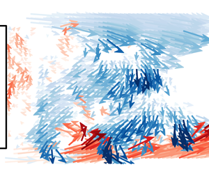
Characteristic wake reversal process exemplified on a natural wake reversal. The reversal is shown by the lateral base CoP position  $y_{b}$. Selected snapshots are indicated by triangles and separated in five different phases. The wake snapshots show the velocity vector field coloured by the lateral velocity
 $u_{y}$. Only one in ten vectors is shown for clarity. Large black arrows indicate the main flows.

The dynamics of a natural wake reversal is elucidated in figure 16 through a time sequence of the instantaneous velocity vector field coloured by the lateral velocity  $u_{y}$. These snapshots are sampled from the time sequence acquired during a wake reversal between lateral asymmetric states
 $\boldsymbol{R}$ and
 $\boldsymbol{L}$ at particular instants of clear changes in
 $y_{b}$, depicted by the markers on the time evolution of
 $y_{b}$. The wake reversal can be separated in five phases denoted from (I) to (V) based on the peculiar flow dynamics during each phase. In the phase (I) launching the reversal, the wake is in the state
 $\boldsymbol{R}$ and the recirculating flow (a) resulting from the right shear layer triggers quite strong roll-up of the left shear layer through the interaction mechanism discussed in the previous section. Large-scale vortical structures (b) and (c) are formed in this shear layer in the second and third snapshot of phase (I) associated with the coherent dynamics characterized in § 5. These structures are quite similar to the hairpin vortices described by Dalla Longa et al. (Reference Dalla Longa, Evstafyeva and Morgans2019) at the beginning of a wake reversal captured numerically. For sufficiently strong large-scale roll-up, the yielded flow engulfment (d) in the recirculation region forms a recirculating flow which interacts with the established recirculating flow from the opposite right shear layer during phase (II). Both recirculating flows (a) and (d) originating from the two opposite shear layers interact, which pinches-off the original recirculating flow (a) characterizing the asymmetric state
 $\boldsymbol{R}$. From then on, no coherent flow movement is established in the recirculation region and thus no triggering of the shear-layer roll-up takes place as discussed in previous section from figure 13. This leads to the highly unstable transient symmetric state
 $\boldsymbol{S}_{tr}$ where the wake meanders around
 $y_{b}=0$ with low drag due to the stabilization of the shear layers and the absence of organized recirculating flow motion. As this wake is highly unstable in the absence of a coherent recirculating dynamics, small perturbation of the fluid engulfment (e) through the opposite shear layers instantaneously breaks the equilibrium by triggering the roll-up of one of the shear layers. It should be noted that rare examples of wake reversal with a wake returning to a similar asymmetric state have also been captured. This could suggest the role of inertia of the wake movement from the
 $\boldsymbol{R}$ state to the
 $\boldsymbol{S}_{tr}$ state in the sense it is highly more probable that the perturbation of the
 $\boldsymbol{S}_{tr}$ state will lead to a reversal to the opposite asymmetric
 $\boldsymbol{L}$ state. The small engulfment imbalance
 $(e)$ leads to perturbation and triggering of roll-up in the opposite shear layer (b). This roll-up finally interacts with the left shear layer to definitely form a strong recirculating flow (d) from the left shear layer which ends the wake reversal event in the asymmetric state
 $\boldsymbol{L}$.
Precursory events of the wake reversal. (a) Natural wake reversal realization presenting a  $\boldsymbol{L}$ to
 $\boldsymbol{R}$ followed by a
 $\boldsymbol{R}$ to
 $\boldsymbol{L}$ reversal. Beginning of each reversal is indicated by the vertical red dashed lines. The average lateral velocity
 $u_{y}^{\unicode[STIX]{x1D6FA}_{L}}$ and
 $u_{y}^{\unicode[STIX]{x1D6FA}_{R}}$ in the symmetric zones
 $\unicode[STIX]{x1D6FA}_{L}$ and
 $\unicode[STIX]{x1D6FA}_{R}$ where interaction between the recirculating flow and the opposite shear layer occurs in asymmetric states is monitored. Blue part of the velocity signal show the precursory important oscillations of the interaction mechanism. (b) Representative snapshots of velocity field coloured by
 $u_{y}$ for extremal
 $u_{y}^{\unicode[STIX]{x1D6FA}_{L}}$ indicated in (a) by the triangles before a reversal. (c) Scalogram of
 $u_{y}^{\unicode[STIX]{x1D6FA}_{R}}$ and
 $u_{y}^{\unicode[STIX]{x1D6FA}_{R}}$ represented by the norm of their wavelet transform
 $|{\mathcal{W}}_{u_{y}^{\unicode[STIX]{x1D6FA}_{R}}}|^{2}$ and
 $|{\mathcal{W}}_{u_{y}^{\unicode[STIX]{x1D6FA}_{L}}}|^{2}$.

As seen from the wake reversal dynamics, the initial triggering of the reversal needs a strong enough recirculating flow to sufficiently trigger the shear layer and create a fluid engulfment able to disconnect the recirculating flow. In figure 17, we present the typical precursory event leading to the triggering of a wake reversal. To underline the generality of this precursory event, it is exemplified on a realization where two consecutive wake reversals are observed, from  $\boldsymbol{L}$ to
 $\boldsymbol{R}$ and then from
 $\boldsymbol{R}$ to
 $\boldsymbol{L}$. All the wake reversals captured present systematically the same precursory event triggering the reversal. In figure 17(a) different time series of the lateral position of the CoP
 $y_{b}$ and averaged lateral velocities over the preferential region of interaction
 $u_{y}^{\unicode[STIX]{x1D6FA}_{L}}$ and
 $u_{y}^{\unicode[STIX]{x1D6FA}_{R}}$ are shown. Both wake reversals are preceded by strong fluctuations of the recirculating flow in the interaction region (either
 $u_{y}^{\unicode[STIX]{x1D6FA}_{L}}$ in the
 $\boldsymbol{R}$ state or
 $u_{y}^{\unicode[STIX]{x1D6FA}_{R}}$ in the
 $\boldsymbol{L}$ state). These fluctuations are quite similar to the ones monitored by Dalla Longa et al. (Reference Dalla Longa, Evstafyeva and Morgans2019) but their interpretation is relatively different. These fluctuations exhibit a relative periodicity which can be elucidated using wavelet transform of the time series. In figure 17(c), the time-resolved frequency content of the fluctuations
 $u_{y}^{\unicode[STIX]{x1D6FA}_{R}}$ and
 $u_{y}^{\unicode[STIX]{x1D6FA}_{L}}$ is provided through the norm of their continuous wavelet transform
 $|{\mathcal{W}}_{u_{y}^{\unicode[STIX]{x1D6FA}_{R}}}|^{2}$ and
 $|{\mathcal{W}}_{u_{y}^{\unicode[STIX]{x1D6FA}_{L}}}|^{2}$. The continuous wavelet transform is estimated by convolution of the fluctuations
 $u_{y}^{\unicode[STIX]{x1D6FA}_{R}}$ with regular complex Morlet wavelets which allows for the best results. A peak around
 $St_{W}\sim 0.1$ is found just before the first wake reversal. Conversely, a similar peak in
 $|{\mathcal{W}}_{u_{y}^{\unicode[STIX]{x1D6FA}_{L}}}|^{2}$ is also found just before the second wake reversal. This
 $St_{W}$ is quite in agreement with the low frequency dynamics dominating the recirculating flow discussed from figure 10. In this sense, it suggests how the opposite shear layer is strongly triggered by the recirculating flow just before the wake reversal. This mechanism is pictured in figure 17(b) where two snapshots are shown corresponding to the local maximum and minimum of
 $u_{y}^{\unicode[STIX]{x1D6FA}_{L}}$ indicated by the orange filled triangles in figure 17(a) just at the onset of wake reversal. In the process, the strong recirculating flow is established at minimal interaction (associated with minimal fluctuations
 $u_{y}^{\unicode[STIX]{x1D6FA}_{L}}$). Once the shear layer has been triggered by this flow at maximal interaction, all the recirculating flow is rolled-up with the shear layer to form the large-scale structures which are triggering the wake reversal by flow engulfment to form the opposite recirculating flow. The knowledge of these precursory events could allow us to predict the onset of wake reversal and make favourable their control by anticipating the event.
7 Discussion and concluding remarks
We summarize the main mechanisms of asymmetry-related drag and wake reversals. The aim is twofold: to interpret a broad range of important results from previous studies through the new insights provided here, and to discuss potential efficient control methods for stabilizing a symmetric wake for drag reduction.
7.1 Flow dynamics in asymmetric and transient states
A conceptual scenario for the near-wake dynamics of asymmetric states is sketched in figure 18. The scenario partly builds on the mechanism proposed by Gerrard (Reference Gerrard1966) for the formation of the recirculation region behind two-dimensional (2-D) bluff bodies through flow entrainment by the surrounding shear layers. Although the present flow configuration is highly three-dimensional (3-D) (Pavia et al. Reference Pavia, Passmore, Varney and Hodgson2020), which cannot be completely neglected, the interaction of opposite shear layers is an important feature of this flow configuration. Grandemange et al. (Reference Grandemange, Gohlke and Cadot2013b) have shown the existence of global instabilities related to the interaction of opposite shear layers in the wake of the Ahmed body, similarly to the global instability in 2-D wakes but with the notable difference that these interactions are less strong. Moreover, Lorite-Díez et al. (Reference Lorite-Díez, Jimenéz-González, Pastur, Martńez-Bazán and Cadot2020) have recently successfully applied the flow description of Gerrard (Reference Gerrard1966) concerning the momentum budget of the wake to the wake of an Ahmed body. Such a description can thus provide important insights about the main mechanisms involved. Four different sub-mechanisms are entangled with each another.
Conceptual scenario of the asymmetry-related drag mechanism. The recirculating flow (a) issued from the stable curved shear layer interacts with the opposite shear layer near the base. The interaction triggers the roll-up of the shear layer (b) and the formation of large-scale vortical structures promoting the engulfment of fluid (c) inside the wake. The increased recirculating flow (d) fed by the fluid engulfment (c) leads to pressure decrease in the wake and on the base.

(I) The asymmetric wake, no matter its orientation, yields an imbalance between opposite shear layers in the direction of the asymmetry. One shear layer has small curvature whereas the opposite one high curvature leading to its stabilization and the formation of a coherent strong recirculating flow (a). This recirculation flow has fundamental importance in the mechanism as it allows feedback in the wake through its interaction with the opposite shear layer.
(II) The interaction mechanism between the recirculating flow (a) formed by one shear layer with the opposite one takes place near the initial development of the shear layer with small curvature. It triggers the shear layer (b), which can be seen as an external forcing of the shear layer. This leads to a strong increase in growth of this shear layer, but also more importantly to its roll-up forming large-scale coherent structures with characteristic scale  $St_{C}\sim 1$ where
 $C$ is the characteristic cross-flow length scale in the direction of the wake asymmetry (i.e. the distance between the shear-layers of interest). At this point the difference between opposite shear layers is quite great due to this feedback interaction.
(III) The strong roll-up of the shear layer (b) results in its nonlinear development and further subharmonic interaction which forms increasingly coherent and strong vortical structures. This yields an engulfment flow (c) which has complementary consequences. For one thing, the flow entrained in the wake by large-scale engulfment feeds the recirculating region. For another thing, the roll-up promotes the asymmetric recirculating flow (a) by induction. This promotes the asymmetry locking as long as the engulfment flow (c) is not too strong. Finally, as discussed by Gerrard (Reference Gerrard1966), the recirculation length  $L_{r}$ shrinks down by a relatively small amount, which is partially related to the increase of base drag in presence of large-scale asymmetries.
(IV) The increased flow inside the recirculating region (d) noticed in asymmetric states stems from the feeding by entrainment flow (c). This enhanced recirculating flow yields a lower pressure at the centre in the toroidal low pressure structure described by Dalla Longa et al. (Reference Dalla Longa, Evstafyeva and Morgans2019). In consequence the pressure imprint on the base is also lowered and the base drag is increased.
The same mechanism is at the origin of wake reversals in bi-modal wakes. The coupled dynamics of the recirculating flow triggering the shear layer and the roll-up of the shear layer leading to engulfed flow promoting and feeding the recirculating flow is the key process leading to wake reversal. When sufficient flow is engulfed, the feedback recirculating flow (a) can impose strong triggering on the opposite shear layer. Then the roll-up of the shear layer (b) gets strong enough to form an opposite recirculating flow which pinches off the main recirculating flow (a) and its feedback necessary to maintain the asymmetry. As a consequence, the wake is brought into a symmetric transient unstable state where both opposing recirculating flows have cancelled each another. This leaves the transient symmetric recirculating wake in a state where no coherent recirculating motion is established. The consequences are twofold: shear layers are not triggered by the recirculating flow which inhibits their growth, and the absence of coherent and organized recirculating motion leads to a higher static pressure in the near-wake flow. This also accounts for the lower pressure drag observed even in asymmetric transient states during wake reversals as a similar disorganization of the recirculating flow occurs.
7.2 On drag changes of wakes influenced by ground clearance
Interpretation of the changes in pressure drag  $\overline{C_{pb}}$ for vertical asymmetric wakes. Left: Evolution of
 $C_{pb}$ with the underbody mass flow rate
 $q$ adapted from Szmigiel (Reference Szmigiel2017). Data from Szmigiel (Reference Szmigiel2017) and Castelain et al. (Reference Castelain, Michard, Szmigiel, Chacaton and Juvé2018) correspond to a modified Ahmed body with aspect ratio
 $H/W=1.12$, fixed ground clearance and pressure losses in the underbody to change
 $q$. Castelain et al. (Reference Castelain, Michard, Szmigiel, Chacaton and Juvé2018) identified four different flow classes depending on the value of
 $q$, and qualitative collapse with the experiments of Grandemange et al. (Reference Grandemange, Gohlke and Cadot2013a) on a canonical Ahmed body has been assessed by Szmigiel (Reference Szmigiel2017). Right: Flow classes (II), (III) and (IV) with important
 $q$ can be ranked as having different degree of interaction between the recirculating flow (a) fed by the bottom shear layer and the top shear layer (b) as sketched following the PIV measurements of Grandemange et al. (Reference Grandemange, Gohlke and Cadot2013a) and Castelain et al. (Reference Castelain, Michard, Szmigiel, Chacaton and Juvé2018). The resulting changes in engulfment flow
 $(c_{II})<(c_{IV})<(c_{III})$ can qualitatively explain the base drag changes for these flows
 $-\overline{C_{pb_{II}}}<-\overline{C_{pb_{IV}}}<-\overline{C_{pb_{III}}}$.

Based on the mechanism described, results of the recent literature about vertical asymmetric wakes may also be interpreted. The changes in underbody flow and in interaction with the ground investigated especially by Grandemange et al. (Reference Grandemange, Gohlke and Cadot2013a), Szmigiel (Reference Szmigiel2017) and Castelain et al. (Reference Castelain, Michard, Szmigiel, Chacaton and Juvé2018) have a strong impact on the vertical asymmetry of the wake and on the base drag generated by the body. These base drag changes may be interpreted using the same asymmetry-related drag mechanism described here. To do so, figure 19 reproduces an important result of Szmigiel (Reference Szmigiel2017) where comparison between different experiments of the evolution of mean base drag  $\overline{C_{pb}}$ with underbody mass flow rate
 $q/(HU_{0})$ is performed. (The experiments of Grandemange et al. (Reference Grandemange, Gohlke and Cadot2013a) and Cadot et al. (Reference Cadot, Evrard and Pastur2015) use a regular Ahmed body with aspect ratio
 $H/W<1$ where the ground clearance is changed to impact the underbody flow rate. Those of Szmigiel (Reference Szmigiel2017) and Castelain et al. (Reference Castelain, Michard, Szmigiel, Chacaton and Juvé2018) use a modified Ahmed body with aspect ratio
 $H/W>1$, fixed ground clearance and side skirts closing the underbody where different perforated plates change the underbody mass flow rate.) The main result of Castelain et al. (Reference Castelain, Michard, Szmigiel, Chacaton and Juvé2018) is the identification of four very different flow classes depending on the underbody mass flow rate which have quite different base drag. If we focus on the three flow classes concerning the highest underbody mass flow rate, a basic sketch of the mean flow topology focusing on the direction of vertical asymmetry is provided in figure 19 based on the flow measurements in Castelain et al. (Reference Castelain, Michard, Szmigiel, Chacaton and Juvé2018) and Grandemange et al. (Reference Grandemange, Gohlke and Cadot2013a). (The first class at low mass flow rates is actually more reminiscent of the flow around a 3-D step on the ground whereas the three other flow classes allow for enough underbody mass flow rate to have a regular 3-D bluff body flows with four shear layers surrounding the recirculation region.) The main criterion proposed by Castelain et al. (Reference Castelain, Michard, Szmigiel, Chacaton and Juvé2018) to discriminate between these different flow classes is the mean curvature of the underbody flow (the flow noted (a) in figure 19). The interaction of the underbody flow with the top shear layer is rather different between the three flow classes. For class (II), almost no interaction occurs as the flow (a) is impinging on the base of the body and the top shear layer develops quite linearly (b) with resulting low large-scale entrainment flow (c) inside the recirculating wake. On the contrary, for flow class (III), the flow (a) directly impinges quasi-normally the upper shear layer with quite an important momentum. This flow (a) has the maximal mean curvature and as such it is strongly stabilized and keeps this important momentum. The high degree of interaction with the top shear layer leads to a strong roll-up (b) and the highest engulfment flow (c). Finally for the flow class (IV) which is equivalent to the vertical asymmetric state
 $\boldsymbol{B}$, the degree of interaction is more moderate both because the recirculating flow (a) is not resulting from ground detachment and thus keeps lower momentum at the interaction location and because the interaction orientation is less normal. This degree of interaction is in agreement with the strength of the Reynolds stresses in the top shear layer systematically measured by Szmigiel (Reference Szmigiel2017). In consequence, the three flow classes can be ranked based on the degree of interaction, of top shear layer destabilization, and of importance of the large-scale flow engulfment as
 $(c_{II})<(c_{IV})<(c_{III})$. Following the asymmetry-related drag mechanism we introduced, the flow classes are ranked in terms of base drag
 $-\overline{C_{pb_{II}}}<-\overline{C_{pb_{IV}}}<-\overline{C_{pb_{III}}}$, which is in qualitative agreement with the measured base drag values provided in figure 19. Legitimately, it can be argued that an important part of the generated base drag comes from the flow curvature of the near wake at first order. However the importance of the asymmetry-related drag mechanism and how it manifests at quite different degrees in these wakes seem fundamental to explain second-order base drag variations among these wakes which represent only 10 % to 20 % of the total base drag.
7.3 Insights into control of wake asymmetries for drag reduction
Finally, the discussion is ended by the implications between wake asymmetries and their control for drag reduction. In the recent literature numerous studies have focused on trying to control and mitigate the asymmetries in the wake of the Ahmed body to reduced its base drag. However, most of the control strategies developed had only mitigated results both in terms of stabilizing the symmetric low drag state  $\boldsymbol{S}_{tr}$ and in terms of drag reduction. The efficacy of all the control strategies targeting the flow asymmetries of the Ahmed body may be interpreted through the asymmetry-related drag mechanism studied previously. A conceptual interpretation of all these control strategies is sketched in figure 20, which the rest of the discussion is based on.
Interpretation of control method efficacy to symmetrize the wake of the Ahmed body with concomitant drag reduction. Passive control methods as a sufficiently deep cavity at the base like in Evrard et al. (Reference Evrard, Cadot, Herbert, Ricot, Vigneron and Délery2016) and Lucas et al. (Reference Lucas, Cadot, Herbert, Parpais and Délery2017), or a spanwise control cylinder in the middle of the recirculation region like in Grandemange et al. (Reference Grandemange, Gohlke and Cadot2014b) are able to satisfactorily suppress the lateral bi-stability by locking the unstable symmetric  $\boldsymbol{S}_{tr}~\text{m}$ode and non-trivially decrease the base drag. This is achieved by preventing the interaction between the recirculating flow (a) and the shear layer (b). Active control methods involving steady and periodic blowing along the edges of the base (see details in the text for the references) can only act on the engulfment flow (c) without preventing the recirculation flow (a) to interact with the shear layer (b). This explains the lack of control authority of these methods for the symmetrization of the wake and the reduction of asymmetry-related drag.

Concerning the mitigation of the bi-modal dynamics and the stabilization of the transient symmetric state  $\boldsymbol{S}_{tr}$ which has received much of the attention lately, control strategies can be separated in three groups depending on the degree of stabilization and drag reduction they achieved. The efficacy of these control strategies to stabilize the wake is directly linked to the degree at which the interaction between the recirculating flow coming from one of the shear layers and the opposite shear layer is prevented.
(i) The passive cavity at the rear base is maybe the most enlightening case. The cavity was shown by Evrard et al. (Reference Evrard, Cadot, Herbert, Ricot, Vigneron and Délery2016) and Lucas et al. (Reference Lucas, Cadot, Herbert, Parpais and Délery2017) to completely stabilize the symmetric low drag state of the wake under the condition the cavity was deep enough. The minimal cavity depth to achieve total stabilization of the symmetric low drag state was found to be
 $0.25H$ which is in good quantitative agreement with the preferential location of the interaction of the recirculating flow with the opposite shear layer identified in our present study. This means that the cavity is able to stabilize the low drag symmetric state on the condition that it completely prevents the feedback from the recirculating flow in the asymmetry-related drag mechanism. The associated base drag decrease is quite important, approximately 9 %, but part of it is ascribed to the artificial elongation of the recirculation region due to the cavity depth.
(ii) The small vertical control cylinder used by Grandemange et al. (Reference Grandemange, Gohlke and Cadot2014b) on the bi-modal Ahmed body wake was only partially able to stabilize the wake in the unstable symmetric low drag state when placed in the vicinity of the middle of the recirculation region. This position appears as the only one where the cylinder hinders the feedback of the asymmetric recirculating flow. Nevertheless due to the small size of the cylinder, it only partially prevents the recirculation interaction. The wake still meanders around the most probable symmetric low drag state with almost similar amplitude as the bi-modal wake and the associated base drag decrease is only small, around 4 %, compared to the 8 % to 10 % identified in the present study. A similar more efficient strategy to prevent the feedback recirculating flow may be to use a splitter plate, as in the 2-D bluff body study of Bearman (Reference Bearman1965), with characteristic length of half of the wake length approximately.
(iii) Active control strategies were used by Li et al. (Reference Li, Barros, Borée, Cadot, Noack and Cordier2016) and Brackston et al. (Reference Brackston, de la Cruz, Wynn, Rigas and Morrison2016) respectively with pulsed jets at the side edges of the base and flapping side flaps to stabilize the bi-modal wake of the Ahmed body. Both studies used closed-loop control based on feedback of the lateral position of the wake
$y_{b}$ and showed how a pseudo-alternate left and right actuation could partially stabilize the symmetric state. However, Li et al. (Reference Li, Barros, Borée, Cadot, Noack and Cordier2016) showed that the best forcing frequency to trigger the shear layer on each side and have enough authority to stabilize the symmetric state of the wake was around $St_{W}\sim 1$ which is the roll-up mode identified in the present study triggered by the recirculation flow feedback. In this sense, the control needed to force the wake reversal mechanism identified here by promoting the roll-up of the shear layer. In consequence, the wake was just meandering around the symmetric state by alternatively forcing the wake reversal mechanism on each side. In addition, the symmetric state which was explored by the wake was a higher drag version of the $\boldsymbol{S}_{tr}$ state as the important flow engulfment promoted by the forcing leads to important organization of the recirculating flow. This is why these two studies only reported a mitigated 2 % of base drag decrease. Using these strategies, only the wake reversal mechanism is triggered, but nothing prevents the recirculating flow to develop and establish the feedback mechanism triggering one of the shear layers. In this sense, the wake can only meander around the symmetric state but never be stabilized in it.(iv) Finally, homogeneous forcing around the whole base either with steady blowing or high frequency blowing is not a fluidic equivalent of the base cavity. The studies of Barros (Reference Barros2015), Lorite-Díez et al. (Reference Lorite-Díez, Jimenéz-González, Pastur, Martńez-Bazán and Cadot2020) or the results presented in Haffner (Reference Haffner2020) show that this type of forcing does not influence the lateral bi-modal dynamics of the Ahmed body wake. The jets exiting at the base only keep momentum for a small streamwise extent after being injected (typically
$0.1H$) before being dissipated by the surrounding flow. In this sense they do not act like a fluidic curtain equivalent to cavity hindering the feedback interaction of the recirculating flow. They only have a certain authority to slightly stabilize the shear layers.


All these flow control results and their interpretation based on the asymmetry-related drag mechanism studied here show that the efficacy of a flow control strategy to stabilize the low drag symmetric state is conditioned on the necessity of preventing the feedback mechanism between the recirculating flow issuing from one shear layer and the opposite shear layer. Control strategies should target the inner region of the recirculation zone to this purpose, because it appears as the region where the symmetry-breaking instability takes its root.
Acknowledgements
The authors would like to warmly thank J.-M. Breux for invaluable support during the experiments, as well as F. Paillé, P. Braud and R. Bellanger for assistance with the aerodynamic balance and the PIV set-up, and P. Sujar-Garrido and M. Michard and for insightful discussions. We thank D. Barros and V. Parezanovic for kindly sharing the flow visualizations used in § 5. We are indebted to the French Agence Nationale pour la Recherche (ANR) through the ANR project Activ_ROAD (ID ANR-15-CE22-0002) and the CPER Feder programme Transport for financial support and would like to thank our project academic partners from Laboratoire Ampère at INSA Lyon and industrial partners PSA Group and Volvo Trucks.
Declaration of interests
The authors report no conflict of interest.
Supplementary movies
Supplementary movies are available at https://doi.org/10.1017/jfm.2020.275.



