I. INTRODUCTION
A lot of research works have been carried out in the past few decades on different antenna arrays in order to get improved radiation pattern. There are several parameters by varying which the radiation pattern can be modified. These parameters are geometrical configurations (e.g. linear, circular, planar, spherical etc.), inter-element spacing, individual excitations (amplitude and phase), and relative pattern of individual elements [Reference Ballanis1, Reference Elliott2]. The goal in such antenna array geometry synthesis techniques is to determine the physical layout of the array that produces the radiation pattern closest to the desired pattern. As the shape of the desired pattern can vary widely depending on the application, many synthesis methods coexist.
Time modulated linear antenna arrays attracted the antenna designers for their advantages over conventional array antennas for a few years. Previous research works have shown time modulated linear antenna arrays are attractive for the synthesis of low/ultralow sidelobes [Reference Shanks and Bickmore3–Reference Zhu, Yang, Zheng and Nie11]. As compared with conventional antenna arrays, the time-modulated antenna arrays introduce a fourth dimension—time—into the design. Consequently, it has more flexibility. While conventional antenna arrays can be considered as the radiation source distributions in space, usually of three-dimensions [Reference Ballanis1, Reference Elliott2]. Consequently, the antenna array cost is tremendously high, which makes it unaffordable for commercial and industrial applications. Therefore, it is naturally necessary to introduce an additional degree of design freedom, a fourth dimension, into conventional antenna arrays, which is so often called in literature as “time”.
In 1959 H. E. Shanks and R. W. Bickmore [Reference Shanks and Bickmore3] published a paper and proposed to use time as a design parameter so as to provide an additional degree of freedom. This technique, which consists of modulating the array elements with a periodic signal shape (in general switching “ON” or switching “OFF” of the array elements), is called time modulation (TM). The concept of the “four-dimensional antenna” can be dated back to as early as 1950s. Thus, the four-dimensional (4D) antennas are also termed as the “time-modulated antenna” in the literature. In 1963, W. H. Kummer et al. extended the concept of 4D antennas to antenna arrays [Reference Kummer, Villeneuve, Fong and Terrio4]. The TM was fulfilled by simple on-off switching of antenna elements in a predetermined sequence, so that, after the antenna output has been filtered, the resulting pattern will have reduced side lobes. There are less stringent constraints on the antenna array errors, while only ordinary side lobes for the static array are required, thus the cost was reduced dramatically. In 1983, Lewis et al. introduced another technique to reduce the signal response entering the antenna array side lobes [Reference Lewis and Evins5]. The essence of Lewis’ idea is that, by moving the phase center of a phased array antenna in the plane of the aperture, signals radiated and received through the antenna side lobes can be shifted out of the pass band of the electronic system receiver, due to Doppler shift effect The phase center motion is achieved by illuminating only part of the total array elements and moving the illuminated part across the entire array electronically, which is apparently not convenient in practical implementation. Moreover, there are no experimental results to verify the theory.
There is a fundamental problem associated with time-modulated linear arrays which is that they generate harmonics, or sidebands at multiples of the switching frequency. Unfortunately the undesirable sideband radiations (SR) represent non-negligible loss of radiated power. These harmonics are generally unwanted as they waste energy and may cause interference in other parts of radio spectrum. Much of the recent research into time-modulated arrays has investigated techniques for reducing the wasted power radiated into sidebands, often by employing various adaptive optimization techniques [Reference Yang, Gan and Qing6–Reference Yang, Gan, Qing and Tan9]. Although in many applications the harmonics generated by time-modulated arrays are unwanted, in certain situations they can be exploited.
In 2002, Yang et al. [Reference Yang, Gan and Qing6] suppressed the SRs of a time-modulated linear array (TMLA) via differential evolution (DE) algorithm by directly optimizing the switch-on time instants. Multiple researches on TMLAs have followed this work. Yang et al. carried out a series of studies on 4D antenna arrays including various features mentioned in [Reference Yang, Gan and Qing6, Reference Yang, Gan, Qing and Tan9–Reference Yang, Gan and Tan12]. All the studies mentioned above demonstrate that the 4D antenna array is a promising candidate for realizing higher performance antenna array with lower cost. The research on TM usually deals with fully filled arrays in which all elements are active.
A concentric circular antenna array (CCAA) [Reference Das13–Reference Haupt19] is a planar array that consists of one or more concentric rings, each having equally spaced array elements on its circumference. An important property of a concentric circular antenna (CCA) is that, its beam pattern remains invariant for 360° azimuthal coverage if the array consists of several rings with an appreciably large number of elements in each ring. Its main attraction is the cylindrical symmetry of its radiation pattern and compact structure, thus finding considerable interest in various applications including radio direction finding [Reference Ballanis1], radar [Reference Munson, O'Brian and Jenkins20], communication [Reference Compton21], and electronic countermeasures, navigation and imaging [Reference Haykin, Justice, Owsley, Yen and Kak22].
Different evolutionary algorithms, genetic algorithm [Reference Haupt19, Reference Panduro, Mendez, Dominguez and Romero23, Reference Panduro, Brizuela, Balderas and Acosta24] particle swarm optimization (PSO) [Reference Panduro, Brizuela, Balderas and Acosta24–Reference Mandal, Ghoshal and Bhattacharjee28], and DE [Reference Yang, Gan and Qing6, Reference Zheng, Yang, Zhu and Nie29, Reference Storn and Price30] have been used in the process of low side lobe array pattern synthesis of CCAA. Some modifications have also been done in the classical DE to increase the performance as modified DE algorithm [Reference Reddy, Bharath, Sahoo, Sinha and Reddy31], and self-adaptive DE algorithm [Reference Chattopadhyay, Sanyal and Chandra32]. DE algorithm is very much sensitive to the choice of control parameters. DE in combination with PSO (DEPSO) [Reference Zhang and Xie33, Reference Hao, Guo and Huang34] is used so as to overcome their individual disadvantages [Reference Kennedy and Eberhart25–Reference Storn and Price30]. Most of the above algorithms show the problems of fixing algorithm's control parameters, premature convergence, stagnation, and revisiting of the same solution over and again. In order to overcome all these problems, the proposed algorithm, known as adaptive fitness based DEPSO (ADEPSO), utilizes the fitness based adaptive differential information obtained from adaptive DE (ADE) [Reference Ghoshal, Giri, Chowdhury, Das and Abraham35, Reference Vasundhara, Kar and Ghoshal36] as well as the memory information obtained from PSO. ADEPSO helps the particles to avoid local minima, sub-optimality, and stagnation problem by increasing the population diversity through the combination of PSO operator with the fitness based ADE operator [Reference Ghoshal, Giri, Chowdhury, Das and Abraham35, Reference Vasundhara, Kar and Ghoshal36]. In this work, this proposed algorithm is employed for the design of TMCCAA. In this work, for simultaneous reduction of side lobe reduction as well as improvement in directivity of the uniformly excited time-modulated CCAA (TMCCAA) [Reference Zheng, Yang, Zhu and Nie29] ADEPSO [Reference Ghoshal, Giri, Chowdhury, Das and Abraham35, Reference Vasundhara, Kar and Ghoshal36] is applied. The statistical analysis and t-test [Reference Walpole and Myer37] have been done to prove the performance of ADEPSO.
The rest of the paper is arranged as follows. In Section II, the design equations for TMCCAA are formulated. Section III briefly discusses about the different evolutionary algorithms, PSO, ADE, DEPSO, and the proposed ADEPSO employed for the TMCCAA design. Section IV describes the simulation results obtained by employing various other evolutionary approaches (PSO, DE, ADE, DEPSO), compared with the proposed ADEPSO based ones. Section V shows the convergence profiles of all the algorithms employed. Finally, Section VI concludes the paper.
II. DESIGN EQUATIONS
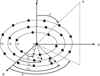
Geometrical configuration is a key factor in the design process of an antenna array. For CCAA, the elements are arranged in such a way that all the antenna elements are placed in multiple concentric rings, which differ in radii and number of elements Fig. 1 shows the general configuration of CCAA with P concentric circular rings, where the pth (p = 1, 2, . . . , P) ring has a radius r p and the corresponding number of elements in the ring is N p . If all the elements in all the rings are assumed to be isotopic sources, the radiation pattern of this array can be written in terms of its array factor (AF) only.
Concentric circular antenna array (CCAA).

Referring to Fig. 1, the AF(θ, ϕ, I) for the CCAA in x–y plane may be written as [Reference Ballanis1]:
 $$\eqalign{&AF(\theta, \phi, I) = 1 \cr & \quad+ \sum\limits_{p = 1}^P {\sum\limits_{i = 1}^{N_p} {I_p \exp [j(kr_p \sin \theta \cos (\phi - \phi _{pi} ) + \alpha _{pi} )]}}, }$$
where I p (I p = 1, throughout this study) is the excitation amplitude of an element on the pth circular ring; k = 2π/λ; λ being the signal wave-length. θ and ϕ symbolize the zenith angle from the positive z-axis and the azimuth angle from the positive x-axis to the orthogonal projection of the observation point, respectively. It may be noted that if the azimuth angle is assumed to be 0° i.e. ϕ = 0°, (1) may be written as an aperiodic function of θ with a period of π radian. The angle ϕ pi is the element-to-element angular separation measured from the positive x-axis. The elements in each ring are assumed to be uniformly distributed.
 $$\phi _{pi} = 2\pi \left( {\displaystyle{{i - 1} \over {N_p}}} \right);\quad p = 1, \ldots, P;\quad i = 1, \ldots, N_p. $$
The term α pi is the phase difference among the individual elements in the array, which is a function of angular separation ϕ pi and ring radii r p .
 $$\eqalign{\alpha _{pi} &= - Kr_p \sin \theta _0 \cos (\phi _0 - \phi _{pi} )\quad p = 1, \ldots, P{\rm ;}\cr & \quad i = 1, \ldots, N_p}, $$
where θ 0 and ϕ 0 are the values of θ and ϕ, respectively, where the peak of the main lobe is obtained. In this paper, θ 0 = 0.
The AF(ϕ, I)for the CCAA in x–y plane can be re-written as (4).
 $$AF\left( {\theta, I} \right) = 1 + \sum\limits_{p = 1}^P {\sum\limits_{i = 1}^{N_p} {I_p \exp [jkr_p \sin \theta \cos (\phi - \phi _{pi} )]}}. $$
There are nine rings where radius of the each ring is given by r p = pλ/2; where p = 1,…, P and inter-element spacing in the entire ring is kept as d p = λ/2, then, the number of equally spaced elements in the ring p is given by
 $$N_p = \displaystyle{{2\pi r_p} \over {d_p}}. $$
For the TM, each ring of CCAA is controlled by a high speed periodic radio frequency (RF) switch U p (t) [Reference Shanks and Bickmore3]. The periodic switch-on time sequence function is given by
 $$U_p (t) = \left\{ \matrix{1\quad {\rm for}\;0 \le t \le {\tau} _p \hfill \cr 0\quad {\rm others} \hfill} \right..$$
Suppose, the array operates at the operating frequency f 0 (Hz) and T 0 is the time period of the operating frequency. TM period of the modulating switch U p (t) is T prf ; hence TM frequency f prf = 1/T prf . Generally the TM frequency f prf is much lower than the operating frequency f 0. It means that T prf > T 0 [Reference Shanks and Bickmore3]. Operating frequency f 0 and TM frequency f prf are independent of each other. Now, instated of exciting each ring continuously, each ring is turned “ON” for the fixed time duration of τ p with a pulse repetition period T prf is lying in the range, τ p ≤ T prf > T 0. Due to RF switch U p (t), the antenna will not only radiate at the operating frequency (f 0) but also will radiate at different harmonics of modulating frequency (f prf ). Harmonics of the radiation pattern are not because of operating frequency of the signal but due to the periodic switch U p (t). An inherent property of time-modulated antenna array is that it generates sideband signals at multiples of TM frequency. It is clear that the sideband radiation (SR) is to be made as small as possible, so that the dynamic mode of the array is the dominant one and the radiation pattern can be controlled without the unwanted SR inconvenience. The simple consideration suggests a way to reduce the amplitude of SR: the higher order harmonics of the Fourier expansion may be lowered by using smoother modulation function. Switch-on time of each ring of TMCCAA is τ p (0 ≤ τ p ≤ T prf ). The far field of TMCCAA is obtained after substituting (6) into (4), which is as follows:
 $$\eqalign{AF(\theta, t) &= e^{j2\pi {f_0}t} \left\{ 1 + \sum\limits_{p = 1}^P \sum\limits_{i = 1}^{N_p} I_p U_p (t) \exp \right. \cr &\quad \times \left. [jk{r_p} \sin \theta \cos (\phi - \phi_{pi})] \right\}}. $$
The periodic switch “ON-OFF” function U p (t) in time domain as represented in (6) can be decomposed into Fourier series in frequency domain, given by
 $$U_p (t) = \sum\limits_{m = - \infty} ^\infty {a_{mp} e^{j2\pi mf_{prf} t}}, $$
where
 $$a_{m{\kern 1pt} p} = \displaystyle{{I_p \tau _p} \over {T_{prf}}} \sin c(mf_{prf} \tau _p )e^{ - j\pi {\kern 1pt} mf_{prf} \tau _p}. $$
Equation (9) shows current excitation value for the mth RF switch modulation frequency. In this work, the authors use (9). m = 0 is for the operating frequency. From (7)–(9), the far field AF can be expanded into Fourier series and given by (10).
 $$\eqalign{AF(\theta ,t) & = \sum\limits_{m = - \infty}^{\infty} \left\{1 + \sum\limits_{p = 1}^P \sum\limits_{i = 1}^{N_p} a_{mp} \exp \right. \cr &\quad \times \left. [jk{r_p} \sin \theta \cos (\phi - \phi_{pi})] \right\} e^{j2\pi (f_0 + m.f_{prf})t}}.$$
The far-field of (10) contains mth harmonic frequency components, m. f prf , where m = 0, ±1, ±2,…, ±∞. It is worth noting that (10) is the sum of infinite number of harmonic components, whose mth order harmonic frequency components can be written as:
 $$\eqalign{A{F_m}(\theta, t) & = {e^{j2\pi ({f_0} + m.{f_{prf}})t}} \left\{1 + \sum\limits_{p = 1}^P \sum\limits_{i = 1}^{N_p} a_{mp} \exp \right. \cr &\quad \times \left. [jk{r_p} \sin \theta \cos (\phi - \phi_{pi})] \right\}}.$$
From (11), one can express the following AFs AF 0(θ, t), AF 1(θ, t), and AF 2(θ, t) for the operating frequency, the first positive side band, and the second positive sideband, respectively.
 $$\eqalign{A{F_0}(\theta, t) & = {e^{j2\pi {f_0}t}} \left\{1 + \sum\limits_{p = 1}^P \sum\limits_{i = 1}^{N_p} {\displaystyle{{{I_p}{\tau _p}} \over {{T_{prf}}}}} \exp \right. \cr &\quad \times \left. [jk{r_p} \sin \theta \cos (\phi - \phi_{pi})] \right\}},$$
 $$\eqalign{AF_1(\theta, t) & = {e^{j2\pi ({f_0} + {f_{prf}})t}} \left\{1 + \sum\limits_{p = 1}^P \sum\limits_{i = 1}^{N_p} {\displaystyle{{{I_p}{\tau _p}} \over {{T_{prf}}}}} \sin c (f_{prf} \tau_p) \exp \right. \cr &\quad \times \left. [jk{r_p} \sin \theta \cos (\phi - \phi_{pi})] e^{- j\pi f_{prf} \tau_p}\right\}},$$
 $$\eqalign{AF_2(\theta, t) & = {e^{j2\pi ({f_0} + {2f_{prf}})t}} \left\{1 + \sum\limits_{p = 1}^P \sum\limits_{i = 1}^{N_p} {\displaystyle{{{I_p}{\tau _p}} \over {{T_{prf}}}}} \sin c (2f_{prf} \tau_p) \exp \right. \cr &\quad \times \left. [jk{r_p} \sin \theta \cos (\phi - \phi_{pi})] e^{- j2\pi f_{prf} \tau_p}\right\}}.$$
Thus, (12)–(14) show the respective expressions for AFs at f 0, f 0 + f prf , and f 0 + 2f prf , which can be used to synthesize the desired radiation pattern.
Similar to time-modulated linear arrays [Reference Yang, Gan and Tan12], the directivity of TMCCAA is given by
 $$D_{TMCCAA} = \displaystyle{{\left\vert {AF_0 (\theta _0, \phi _0 )} \right\vert^2} \over {{\textstyle{1 \over {4\pi}}} \sum\nolimits_{m = - \infty} ^\infty {\int_0^{2\pi} {\int_0^\pi {\left\vert {AF_m (\theta, \phi )} \right\vert^2 \sin \theta d\theta d\phi}}}}}, $$
where D TMCCAA is the directivity of the TMCCAA; θ 0 denotes the direction in which AF(θ, ϕ) has maximum value; and AF m (θ, ϕ) denotes the radiation pattern at the mth order sideband frequency. In this paper two sideband frequencies have been taken, so, (15) can be re-written as (16).
 $$D_{TMCCAA} = \displaystyle{{\left\vert {AF_0 (\theta _0, \phi _0 )} \right\vert^2} \over {{\textstyle{1 \over {4\pi}}} \sum\nolimits_{m = 0}^2 {\int_0^{2\pi} {\int_0^\pi {\left\vert {AF_m (\theta, \phi )} \right\vert^2 \sin \theta d\theta d\phi}}}}}. $$
The power radiated by the TMCCAA, P 0 at the fundamental (center) frequency is given by (17)
 $$P_0 = \int_0^{2\pi} {\int_0^\pi {\left\vert {AF_0 (\theta, \phi )} \right\vert^2 \sin \theta d\theta d\phi}}. $$
The power radiated by the TMCCAA, P SR at the harmonic frequency is given by (18).
 $$P_{SR} = \sum\limits_{\scriptstyle m = - \infty, \hfill \atop \scriptstyle m \ne 0 \hfill} ^\infty {\int_0^{2\pi} {\int_0^\pi {\left\vert {AF_m (\theta, \phi )} \right\vert^2 \sin \theta d\theta d\phi}}}. $$
Dynamic efficiency (η d ) is defined as the ratio of power radiated by the array at the center frequency and the sum of powers radiated by the array at the fundamental (center) frequency as well as the harmonic frequencies, given by (19).
 $$\eqalign{& {\eta _d} = \displaystyle{1 \over {1 + \left[ {\left( {\sum\nolimits_{\scriptstyle m = - \infty, \hfill \atop \scriptstyle m \ne 0 \hfill} ^\infty {\int_0^{2\pi} {\int_0^\pi {{{\left\vert {A{F_m}(\theta ,\phi )} \right\vert}^2}\sin \theta d\theta d\phi}}}} \right)} \right.}} \cr & \quad \quad \quad \left. {/\left( {\int_0^{2\pi} {\int_0^\pi {{{\left\vert {A{F_0}(\theta,\phi)} \right\vert}^2}\sin \theta d\theta d\phi}}} \right)} \right]}. $$
The main objective in this paper is to optimize three different control parameters; the first optimizing parameter is the switching time sequence τ p of the each ring. It means each ring will be active for the optimal time obtained by the optimization algorithm. The main benefit of optimizing this additional parameter is better control of the radiation pattern by applying high speed RF switches, even if the excitation amplitude for each ring is made uniform being equal to 1. The second optimizing parameter is radius of each ring (r 1, r 2, …r p ). There should be some constraints as r 1 > 0.5λ, and for the inter-ring spacing as 0.5λ < r p < λ. The third optimizing parameter is inter-element spacing in each ring, and this optimization parameter also follows the minimum constraint of 0.5λ < d p < λ. An additional separation of Δp is added so that
 $$r_{p} = r_{p - 1} + \lambda /2 + \Delta_{p} ;{\rm where}\,\,0 \le \Delta_{p} \le \lambda. $$
After defining the optimizing parameters, the next task is to define the objective/fitness function, which is expressed as follows:
 $${\eqalign{{f_{fitness}^g} (\tau _P, r_p, d_p ) =\cr & {w_{11}}\,^{\ast} {SLL_{\max}^g} (\tau _P, r_p, d_p )\vert_{f_0} + {w_{22}}\,^{\ast} {SBL_{\max}^g} (\tau _P, r_p, d_p )\vert_{f_0 + f_{prf}} \cr & + {w_{33}}\,^{\ast} {SBL_{\max}^g} (\tau _P, r_p, d_p )\vert_{f_0 + 2f_{prf}} \cr & + {w_{44}}\,^{\ast}(1/D_{TMCCA}\_{\rm max}} ),} $$
where g denotes the gth iteration cycle;
 $SLL_{\max} \vert_{f_0} $
is the maximum side lobe level (SLL) at the center frequency;
 $SBL_{\max} \vert_{f_0 + f_{prf}} $
is the maximum sideband level (SBL) at the first sideband frequency;
 $SBL_{{\rm max}} \vert_{f_0 + 2f_{prf}} $
is the maximum SBL at the second sideband frequency, and w
11, w
22, w
33, and w
44 are the weighting factors of various terms to emphasize the different contributions to the fitness function. D
TMCCA_max is the maximum directivity of the TMCCAA.
III. OPTIMIZATION TECHNIQUES EMPLOYED
The PSO [Reference Panduro, Brizuela, Balderas and Acosta24–Reference Mandal, Ghoshal and Bhattacharjee28] and the conventional DE [Reference Zheng, Yang, Zhu and Nie29, Reference Storn and Price30] are well known and hence not discussed here. Only the hybridized DE and PSO are discussed here.
A) Fitness Based ADE
It is known that crossover rate and scaling factor play important roles in the convergence and performance of DE. In this paper, we have tried to use the fitness based ADE, which uses the concept of fitness based variation of crossover rate [Reference Ghoshal, Giri, Chowdhury, Das and Abraham35]. The ADE works with all the same steps of the classical DE as stated in the previous section of classical DE, but the difference lies in the use of fitness based adaptive crossover rate used in the crossover step (b) of classical DE. Instead of constant crossover rate, which is used in classical DE, the value of the crossover rate used in the recombination process to produce the trial vector is adapted according to the fitness value of the donor vector. In this case a vector is created.
 $$\Delta f_{donor\_i} = (f(v_i ) - f(x_{best} )),$$
where f(v i ) is the fitness value of ith donor vector and f(x best ) is the fitness value of the best individual in the population. The value of crossover rate is decided according to this Δf donor_i . If the value of crossover rate is higher, then more information will be passed from the donor vector to the trial vector whereas if the value of crossover rate is lower, then more information will be passed from the target vector to the trial vector.
In this case the donor vectors having lower value of Δf donor_i , are located close to the best particle obtained so far in the current population and hence they prove themselves to be the promising candidates to form the trial vectors than the target vectors. In the same manner the donor vectors having higher value of Δf donor_i are far away from the best candidate and in this case target vectors are to be transmitted in the trial vectors. So, in this case of fitness based ADE, the recombination operation gets modified slightly as:
If f(v i ) < f(x best ), for the minimization process
 $${\rm then}\,Cr_i = Cr\_{\rm const,}$$
 $${\rm else}\,Cr_i = Cr_{{\rm min}} + (Cr_{{\rm max}} - Cr_{{\rm min}} )/(1 + \Delta f_{donor\_i} ).$$
Equation (23) can be analyzed as:
If f(v i ) < f(x best ) for minimization problem or Δf donor_i 0, C ri should have a large value to ensure maximum information transmission from the donor vector to the trial vector. In the same manner when Δf donor_i 0, C ri tends to Cr max and when Δf donor_i ∞, then C ri tends to Cr min ,which is of low value, and ensures minimum information to be transferred from the target vector to the trial vector.
B) DEPSO
The limitations of PSO and DE are that they may be influenced by parameter convergence and stagnation problem. To overcome the problems associated with DE and PSO; both of them can be merged so as to overcome their individual disadvantages. The hybrid of DE and PSO is called DEPSO [Reference Zhang and Xie33]. In DEPSO new offspring is created by the mutation of the parent.
Steps of DEPSO are as follows:
-
• First a population is randomly initialized.
-
• The fitness value of the population is evaluated (21), best among the fitness is considered to be g best.
-
• The velocity and the position of the particles in the search space is evaluated using velocity and position update formula of PSO.
-
• Now the updated population by PSO will be used to employ differential evolution.
-
• Donor vector is created by DE's mutation strategy DE/best/1.
-
• Trial vector is created by crossover process using binomial (uniform) crossover formula of DE.
-
• The fitness value of the trial vector is calculated and the one having the better fitness value among the trial and the target vector is finally taken as the updated population.
C) Fitness based ADEPSO
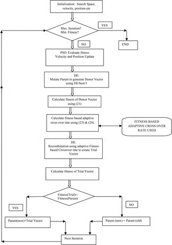
The DEPSO utilizes the benefits incurred in both the algorithms individually. But then also, as far as global optimization is considered, there is still room left for its further improvement over the existing DEPSO approaches in terms of robustness and accuracy of the optimization algorithms. The DEPSO is modified with the use of fitness based adaptive crossover rate used for the crossover purpose, called ADEPSO [Reference Vasundhara, Kar and Ghoshal36]. In classical DE, the crossover rate is fixed, but here the crossover rate is being varied in accordance with the Δf donor_i calculated (23). The one having better fitness value should have more probability of being transferred to the trial vector rather than the one having lower fitness value. So, using this concept crossover rate is calculated separately for each and every element of the population set. The adaptive crossover rate is chosen according to that given in (22) and (23).
The steps for the ADEPSO are written as follows:
-
• Initial particles: Randomly generate the initial population matrix.
-
• Evaluate particles: Calculate the fitness value for each set of particles in the population.
-
• Update global best: Take the particle with the best fitness value or the minimum fitness value since it is a minimization problem as the global best.
-
• Update personal best: Compare the newly calculated fitness value with the previous one for each and every individual and select the one having the better fitness value as the personal best.
-
• Update velocity of the particles: Update velocity of the particles using velocity update formula of PSO.
-
• Update position of the particle: update position of the particles using position update formula of PSO.
-
• Generate donor vector: The updated particles are used for creating the donor vector by DE's mutation strategy DE/best/1.
-
• Calculate fitness value of the donor vectors generated: Calculate the fitness value of the donor vector generated using (21).
-
• Calculate difference vector: The difference vector is created by using (22).
-
• Calculate the fitness based crossover rate: Now the fitness based crossover rate is generated using (23) and (24).
-
• Generate trial vector: The trial vector is created by mutation between donor and target vector using binomial (uniform) crossover formula of DE.
-
• Selection: Among trial and target vector, whichever proves itself to be better candidate in terms of fitness is selected for the final population.
-
• Termination: If the maximum number of iterations is reached or terminating condition is satisfied.
The algorithm of the fitness based ADEPSO can also be summarized in the form of flowchart as shown in Fig. 2
Flowchart showing ADEPSO.

IV. NUMERICAL RESULTS
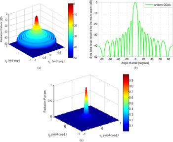
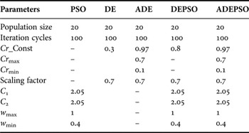
ADEPSO, DEPSO, ADE, DE, and PSO have been each run for 100 times for each case study to get its best solutions. These best parameters have been determined after 50 trial runs of each algorithm, taking all the case studies together. Table 1 shows the control parameters of each algorithm. This section gives the experimental results for various time modulated CCAA designs obtained by each algorithm. Nine-ring (P = 9) TMCCAA structures is assumed. Each algorithm has been implemented to study the behavior of the radiation pattern for the TMCCAA. In this case, the radiation pattern with main lobe steered to θ 0 = 0 degrees is considered. Directivity is calculated numerically by Simpson's 1/3 rule. Velocity of electromagnetic wave in the free space is given by c = 3.0 × 10⁸ m/sec; operating frequency, f 0 = 3.0 GHz; TM frequency, f prf = 1/T prf . TM period of the modulating switch, U i (t) is T prf = 1 µs (Sometimes one can take T prf = max (optimized value of τ p ), then, one can calculate TM frequency, f prf = 1/T prf . Figure 3 show radiation patterns of uniform Nine-ring CCAA: (a) 3D Normalized plot (dB), (b) 2D plot, (c) Un-normalized 3D plot. Table 2 lists the ring spacing and number of elements in each ring (total 279 elements) for the uniform concentric ring array with nine rings. Ring radius, r p = p. λ/2 and inter-element spacing in each ring, d p = λ/2. To keep d p ≥ λ/2 and allow sufficient inter-element spacing, the digits to the right of the decimal point are dropped. Table 2 shows the SLL of −17.4 dB, first null beamwidth (FNBW) of 14.76°, and Directivity (D) of 29.35 for the uniform nine-ring CCAA.
Radiation patterns of uniform nine-ring CCAA: (a) 3D normalized plot (dB), (b) 2D plot, and (c) un-normalized 3D plot.

Control parameters of PSO, DE, ADE, DEPSO, and ADEPSO.

SLL, FNBW, and Directivity of CCAA.

A) Case-1: Optimizing only switching time sequence of each ring
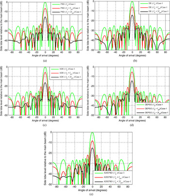
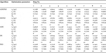
A planar uniform nine-ring CCAA with only TM is considered [Reference Haupt19]. In this example, the uniform array has all throughout equal inter-element spacing of λ/2, inter-ring spacing of λ/2 and uniform amplitude weighting (I P = 1) for each element. The radius of each ring of the array antenna is made equal to 0.5*λ*p, where p is the ring number counted from the innermost ring 1. The total number of isotropic elements including the central element in the array is 279. The analysis for the TMCCAA ring is done only by optimizing switching time sequence of each ring. Table 3 shows the optimal switching time sequence of each ring obtained by PSO, DE, ADE, DEPSO, and ADEPSO. In this study, radius of each ring and number of elements in each ring are kept same as those of the uniform CCAA for the fixed number of elements in each ring. Figure 4 shows radiation patterns obtained by PSO, DE, ADE, DEPSO, and ADEPSO for Case-1.
Radiation patterns obtained for Case-1 by different algorithms: (a) PSO, (b) DE, (c) ADE, (d) DEPSO, and (e) ADEPSO.

Optimizing only switching time sequence of each ring.

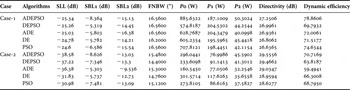
Table 5 also shows SLL, SBL1, SBL2, FNBW, power radiated at the fundamental frequency (P0), power radiated at the first harmonic (P1), and power radiated at the second harmonic (P2), Directivity (D), and dynamic efficiency (η) obtained by different algorithms.
Table 5 shows that for Case-1, SLL, and Directivity obtained by ADEPSO are much better than those obtained by PSO, DE, ADE, DEPSO, and those of the uniform CCAA, with a little increase in FNBW.
B) Case-2: Optimizing switching time sequence, ring radii, and optimal uniform inter-element spacing
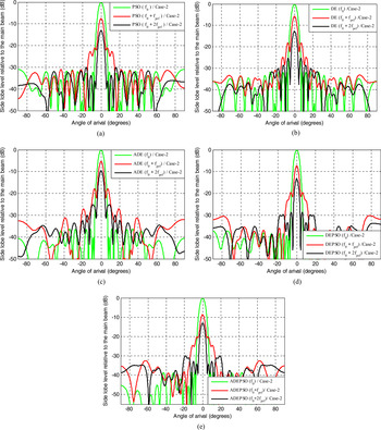
In this case, the best non-uniform switching time sequence τ p of each ring, ring radius r p , and uniform inter-element spacing within the ring d p are determined by PSO, DE, ADE, DEPSO, and ADEPSO. Table 4 shows the optimal values of switching time sequence, optimal ring radii, and optimal uniform inter-element spacing obtained by PSO, DE, ADE, DEPSO, and ADEPSO. Figure 5 shows radiation patterns obtained by RGA, PSO, DE, and DEWM for Case-2.
Radiation patterns obtained for Case-2 by different algorithms: (a) PSO, (b) DE, (c) ADE, (d) DEPSO, and (e) ADEPSO.

Optimizing switching time sequence, ring radii, and optimal uniform inter-element spacing.

From the Table 5, it is observed that (i) all optimal results (regarding SLL, SBL1, SBL2, P0, P1, P2, Directivity, and dynamic efficiency) obtained by using ADEPSO are better than those by PSO, DE, ADE, and DEPSO (except FNBW which has increased a bit for ADEPSO) and (ii) Case-2 yields the best radiation characteristics. Hence, optimizing switching time sequence, optimal ring radii, and optimal uniform inter-element spacing in Case-2 yield the best optimal design of time modulated nine-ring as compared with the designs resulted in the Case-1.
Optimal SLL, SBL1, SBL2, FNBW, P0, P1, P2, Directivity, dynamic efficiency of TMCCAA obtained by PSO, DE, ADE, DEPSO, and ADEPSO algorithms.

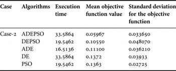
Table 6 shows execution time, mean objective function value, and standard deviation for the objective function for Case-2, obtained by PSO, DE, ADE, DEPSO, and ADEPSO.
Execution times, mean fitness function value, standard deviation for the fitness functions applied for Case-2, obtained by ADEPSO

From the analysis of all the numerical results of the three case studies depicted in Table 5, it is observed that SLL, and Directivity obtained by PSO, DE, ADE, DEPSO, and ADEPSO for Case-2 are much better than those of corresponding PSO, DE, ADE, DEPSO, and ADEPSO for Case-1, and uniform CCAA. ADEPSO also outperforms PSO, DE, ADE, DEPSO, uniform CCAA and, those obtained in [Reference Haupt19, Reference Zheng, Yang, Zhu and Nie29] and with respect to reduced SLL, and directivity with respect to reduced SLL and improved Directivity for all the cases. Again, Case-2 also outperforms Case-1 with respect to FNBW. Figs 4 and 5 and Table 5 show that as the harmonic frequency increases the SBLs decrease. The table shows that sometimes SLL values are higher than SBL1 and SBL2, but the power associated with the fundamental frequency is much higher than the corresponding powers P1 and P2 associated with SBL1 and SBL2, respectively. This means that even though TMCCAA has a drawback of harmonic radiations, powers radiated by the sidebands are very less. So, one can say that ADEPSO for Case-2 gives the best optimal results for TMCCAA. The dynamic efficiency obtained by using ADEPSO for Case-2 is more than 70%, which is well acceptable.
C) Comparisons of accuracy
Test for independent samples is conducted at the 5% significance level in order to judge whether the results obtained with the best performing algorithm differ from the results of the other algorithms in a statistically significant way. Two sample t-test is a hypothesis testing method for determining the statistical significance of the difference between two independent samples of an equal sample size [Reference Walpole and Myer37]. The t-test value will be positive if the first algorithm is better than the second, and it is negative if it is poorer. The t-value is defined as given in the following equation. Assume unequal population variances/standard deviations
 $(\sigma _1^2 \ne \sigma _2^2 )$
. Two sample t-test with equal sample size has been adopted; sample size is 51.
Test statistic is given by
 $$t{\rm - test} = \displaystyle{{\bar \alpha _{22} - \bar \alpha _{11}} \over {\sqrt {\left( {\sigma _2^2 /n_A} \right) + \left( {\sigma _1^2 /n_B} \right)}}}, $$
 $${\rm Degree\,of\,freedom}\,(\beta ) = {\rm min}(n_A - 1,n_B - 1),$$
where
 $\overline \alpha _{11} $
and
 $\overline \alpha _{22} $
are the mean values of the first and the second algorithm, respectively; σ
1 and σ
1 are the standard deviations of the first and the second algorithm, respectively; n
A
and n
B
are the numbers of sample sizes in first and second algorithm, respectively. The degree of freedom for unequal variance and unequal sample size is given by (26). In this paper n
A
= n
B
is taken. Degree of freedom = 50. Table 7 shows t-test and p-value values obtained between the ADEPSO over PSO, DE, ADE, and DEPSO. When the t-test value is higher than 1.676, 2.009, 2.403, 2.678, 2.937, and 3.261 (β = 50), there is a significant difference between the two procedures with 95, 97.5, 99, 99.5, 99.75, and 99.9% confidence levels, respectively [Reference Walpole and Myer37]. The t-test values with the ADEPSO over PSO, DE, ADE, and DEPSO for Case-2 are presented in Table 7. The t-test values of all approaches are larger than 3.261, meaning that there is a significant difference between the ADEPSO over PSO, DE, ADE, and DEPSO with a 99.9% confidence level. Thus, from statistical analysis, it is clear that the ADEPSO offers more robust and promising results.
t-test values and p-values obtained for comparison of ADEPSO with other algorithms for Case-2.

In this paper p-value is using Student's t cumulative distribution function [Reference Walpole and Myer37]. If the p-value is less than the significance level (the default, when unspecified, is α = 0.05) then we can reject null hypothesis, it means that statistical performance of the proposed algorithm is better than that of other algorithms, and we will accept the proposed algorithms, otherwise do not. In general, the statement “one can reject the null hypothesis at the 100(1 − α)% confidence level” is equivalent to the statement “The p-value is equal to α.” From Table 7 it is clear that all p-values obtained for ADEPSO over other algorithms is much lesser then 0.05, which is clear that ADEPSO outperforms PSO, DE, ADE, and DEPSO.
V. COMPARATIVE EFFECTIVENESS AND CONVERGENCE PROFILE OF PSO, DE, ADE, DEPSO, AND ADEPSO
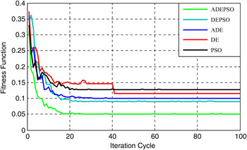
The minimum f fitness values are recorded against number of iteration cycles to get the convergence profiles for fitness function (f fitness ) based on PSO, DE, ADE, DEPSO, and ADEPSO for each optimal array design. Figure 6 portrays the convergence profiles for the Case-2. From Fig. 6 it is clear that ADEPSO gives the better convergence characteristics over PSO, DE, ADE, and DEPSO. The programming was written in MATLAB language using MATLAB 7.5 on dual core (TM) processor, 2.88 GHz with 1 GB RAM.
Convergence profile obtained by PSO, DE, ADE, DEPSO, and ADEPSO for Case-2.

VI. CONCLUSIONS
The comparative performance of pattern synthesis of nine-ring, 279-element TMCCAA in terms of optimal beam pattern and optimal values of SLL, SBLs at its harmonics, FNBW, Directivity, and dynamic efficiency are discussed with two cases, Case-1: optimizing only switching time sequence of each ring; and Case-2: optimizing switching time sequence, ring radii, and uniform inter-element spacing. For optimal radiation pattern, each case is studied by using identical fitness function. The contribution of the paper is twofold: (1) with respect to SLL, FNBW and Directivity, the performance of the ADEPSO proves to be better than that of the PSO, DE, ADE, and DEPSO. (2) Case-2 outperforms Case-1 and uniform CCAA with respect to SLL, FNBW, and Directivity. For statistical analysis, t-test has also been done for the stability of ADEPSO over PSO, DE, ADE, and DEPSO, for Case-2. t-test results show that Case-2 with ADEPSO gives the best performance as compared with the performances of PSO, DE, ADE, and DEPSO. Thus, the numerical results make it clear that for the optimal design of time-modulated antenna arrays, optimizing algorithms, and selection of proper optimizing variables related to the array play important roles. Numerical results show the excellent side lobe control capability for pattern synthesis by using the TM technique. As compared with the method of non-uniform amplitude excitation weighting method, controlling the switch-on time of each element is the best method which can be more precisely and more rapidly realized. From the results, it is also established that powers radiated by the TMCCAA at harmonic frequencies are less as compared with that at the fundamental frequency, even though SBLs of optimal patterns at the harmonic frequencies are lower, sometimes, are higher than SLL of optimal pattern at the fundamental frequency. Again, as the harmonic frequency increases, SBLs decrease. The proposed method is applicable for the design of time-modulated antenna arrays with other geometrical configurations.
 Gopi Ram passed B. E. degree in Electronics and Telecommunication Engineering, from Government Engineering College, Jagdalpur, Chhattisgarh, India in the year 2007. He received the M. Tech degree from National Institute of Technology, Durgapur, West Bengal, India in the year 2011. Presently, he is attached with National Institute of Technology, Durgapur, West Bengal, India, as Institute Ph.D. Research Scholar in the Department of Electronics and Communication Engineering. His research interest includes Array Antenna design; via Evolutionary Computing Techniques.
 Durbadal Mandal passed B. E. degree in Electronics and Communication Engineering, from Regional Engineering College, Durgapur, West Bengal, India in the year 1996. He received the M. Tech and Ph.D. degrees from National Institute of Technology, Durgapur, West Bengal, India in the year 2008 and 2011, respectively. Presently, he is attached with National Institute of Technology, Durgapur, West Bengal, India, as Assistant Professor in the Department of Electronics and Communication Engineering. His research interest includes Array Antenna design; filter Optimization via Evolutionary Computing Techniques. He has published more than 250 research papers in International Journals and Conferences.
 Rajib Kar passed B. E. degree in Electronics and Communication Engineering, from Regional Engineering College, Durgapur, West Bengal, India in the year 2001. He received the M. Tech and Ph.D. degrees from National Institute of Technology, Durgapur, West Bengal, India in the year 2008 and 2011, respectively. Presently, he is attached with National Institute of Technology, Durgapur, West Bengal, India, as Assistant Professor in the Department of Electronics and Communication Engineering. His research interest includes VLSI signal Processing, Filter optimization via Evolutionary Computing Techniques. He has published more than 250 research papers in International Journals and Conferences.
 Sakti Prasad Ghoshal passed B. Sc. and B. Tech. degrees in 1973 and 1977, respectively, from Calcutta University, West Bengal, India. He received M. Tech. degree from I.I.T (Kharagpur) in 1979. He received Ph.D. degree from Jadavpur University, Kolkata, West Bengal, India in 1992. Presently he is acting as Professor of Electrical Engineering Department of N.I.T. Durgapur, West Bengal, India. His research interest areas are: Application of Evolutionary Computing Techniques to Electrical Power systems, Digital Signal Processing, Array antenna optimization and VLSI. He has published more than 270 research papers in International Journals and Conferences.