Cotton, Children, and Schooling

At the beginning of the twentieth century, the South was still an agrarian economy, as agriculture employed 57 percent of the labor force in 1910. And cotton was its staple. Cotton was the single most valuable crop in 10 of the 16 Southern states at the dawn of the twentieth century. In Alabama, Arkansas, Georgia, Mississippi, South Carolina, and Texas—the states that formed the heart of the Cotton Belt—cotton comprised more than half of the value of all crops produced (U.S. Bureau of the Census 1913).

The widespread cultivation of cotton and its long harvest season, which commonly ran from September through December, generated a seasonal increase in demand for labor, as harvesting cotton was not mechanized until the mid-twentieth century. Since harvesting cotton involves repetitively picking lightweight fibers from their bolls and transferring them to a sack, it is a tedious task that is performed reasonably well by anyone over the age of five. In the cotton harvest, therefore, there was a high degree of substitutability between adult and child labor (Bradley and Williamson 1918; Matthews and Dart 1924).Footnote ⁵ It is not surprising, then, that agriculture was by far the largest employer of children. In 1910, 34.4 percent of 10 to 15 year olds living in the South worked, of which 86.7 percent were employed in farming. Moreover, these youth made up 17 percent of the agricultural labor force in the South (U.S. Bureau of the Census 1924).Footnote ⁶ The majority of these child laborers undoubtedly worked the cotton fields.

While some adjustments were made to the school calendar in an attempt to accommodate farming cotton (Collins and Margo 2006), the lengthy harvest period could not be avoided altogether. Baker (Reference Baker2015) provides anecdotal evidence of the conflict between the demand for child labor in farming cotton and schooling in Georgia, but this conflict is not unique to that state. The superintendent of West Baton Rouge Parish, Louisiana, noted, “a falling off in attendance at several schools during the harvesting season … due to the scarcity of labor and the need of the children in the cotton fields” (Louisiana Department of Education 1908, p. 48). His colleague in Calcasieu Parish expressed similar sentiments, observing, “times to pick cotton, the harvesting of rice and other crops take many out of school for a good part of the term” (Louisiana Department of Education 1902, pp. 60–61). To accommodate the surge in attendance following the conclusion of the cotton picking season, the superintendent of Tunica County, Mississippi, planned to hire an additional teacher in each African-American district (Mississippi Department of Public Education 1907, p. 95). Even Texas Superintendent Arthur Lefevre noted, “the average daily attendance being unusually low during 1902–3 on account of the high price and long picking season of the cotton crop of that year” (Texas Department of Education 1905, p. 7).

The Boll Weevil

The adult cotton boll weevil, Anthonomus grandis, is a small beetle, about six millimeters in length, and grayish in color, with a long snout and wings.Footnote ⁷ The westward expansion of cotton production in the United States during the nineteenth century eventually linked the Cotton Belt with the native habitat of the boll weevil, Mexico and Central America. The boll weevil first appeared in cotton fields near Brownsville, Texas, in 1892. It then spread north and east at a steady rate. By 1922, the boll weevil could be found in virtually all cotton counties in the United States, from Texas to North Carolina (Hunter and Coad Reference Hunter and Coad1923).

The life cycle of the boll weevil is closely intertwined with the cotton plant. Indeed, the insect lives inside the squares and bolls of the cotton plant for three of the four stages of its life cycle (egg, larvae, and pupae), and as an adult it feeds almost exclusively on the cotton plant.Footnote ⁸ The reason for the boll weevil’s narrow appetite is that cotton is one of only a few plants (the others being wild flora with geographically small habitats) that provide the weevil with the nutrients required to produce the pheromones necessary for its reproduction. This dependence on cotton causes the insect to spend its entire life in or near cotton fields (Giesen Reference Giesen2011).

The boll weevil’s spread had a disastrous effect on cotton production in the South. Damaged squares and bolls usually dropped from the plant after being fed upon and following the deposition of eggs by the boll weevil. As a result, heavily infested areas saw significant reductions in cotton output. In a county-level analysis, Lange, Olmstead, and Rhode (2009) demonstrate that within five years of the boll weevil’s arrival cotton production fell by approximately 50 percent, due primarily to reduced yield but also reduced cotton acreage.

The boll weevil’s negative effect on cotton yields decreased the returns to farming cotton relative to other crops. This caused farmers to substitute away from cotton in favor of more profitable alternatives, including corn, peanuts, potatoes, and sweet potatoes. These alternative crops generated less demand for child labor than cotton (Bradley and Williamson 1918; Matthews and Dart 1924).Footnote ⁹ Farmers also responded to the boll weevil by growing earlier maturing varieties of cotton and moving up the planting date, as the insect did the most damage late in the season (Lange, Olmstead, and Rhode 2009). This reduced the conflict between the timing of the cotton harvest and fall schooling. Therefore, the arrival of the boll weevil, and the subsequent reduction in cotton production, had significant implications for the whole household.

Mapping the Progress of the Boll Weevil

Information on the presence of the boll weevil was collected from the USDA-produced map tracking the insect’s spread provided by Hunter and Coad (Reference Hunter and Coad1923). For each year from 1892 through 1922 the counties of the Cotton Belt were assessed as being either boll weevil free, partially infested, or fully infested. A county was considered to be partially infested in a given year if and only if the line denoting the frontier of the boll weevil infestation in that year passed through the county leaving parts of the county visible on both sides of the line. Using this panel data, we then define three measures for each county that capture the timing of the arrival of the boll weevil: We define the first arrival year as the first year in which the county is coded as either partially or fully infested. The complete infestation year is the first year in which the county is coded as fully infested and not subsequently found to be boll weevil free or partially infested. The year of infestation is the ceiling of the average of the first arrival year and complete infestation year. We use year of infestation for each county to construct indicators for the presence of and exposure to the boll weevil throughout our analysis, which is consistent with the methodology of Lange, Olmstead, and Rhode (2009).Footnote ¹¹

In our examination of the long-run effects of the boll weevil on education, we restrict our analysis to certain counties based on characteristics of the timing of the boll weevil’s arrival, to increase the precision with which we date treatment. First, we begin with all Southern counties that Hunter and Coad (Reference Hunter and Coad1923) identify as having territory within the Cotton Belt: 993 counties spread over 13 states.Footnote ¹² Second, we exclude 102 counties that were boll weevil free and 47 counties that were only partially infested in 1922, approximately half of which are in the Western High Plains and Southwestern Tablelands regions of Texas and Oklahoma.Footnote ¹³ This restriction limits our sample to 844 counties, across 12 states, of the Cotton Belt that were fully infested by the boll weevil in 1922. Third, we remove counties that experienced a full retreat of the boll weevil (assessed as being boll weevil free in a year subsequent to being partially or fully infested), which drops 120 counties.Footnote ¹⁴ Fourth, we exclude 38 additional counties where the absolute difference between the first arrival year and the complete infestation year is greater than four years; 30 of these are in Texas, 6 in Arkansas, and 2 in Oklahoma.Footnote ¹⁵ Finally, we require that childhood location of individuals in our linked census data be observed prior to the boll weevil’s arrival in that location, to ensure that our results are not biased by weevil induced migration.Footnote ¹⁶ This requirement further excludes from our sample 33 counties, which are all in Texas, where the boll weevil infestation began prior to 1900. This leaves us with a sample of 653 Southern counties across 12 states.Footnote ¹⁷

Linked Census Data

We start by extracting all men born in the 13 Southern states of the Cotton Belt from the 1940 full count census data, provided by IPUMS and accessed through the NBER server. Then, we link these men to themselves as children in the 1900, 1910, or 1920 censuses. We restrict our search to individuals who were between the ages of 3 and 18 in the earlier census years; this means that they were between 23 and 58 years old in 1940.Footnote ¹⁸ In the case where men are found as children in two census years, we keep the earlier observation.Footnote ¹⁹

We link individuals on the basis of first name, last name, birth year, race, and birth state using the standard procedure developed by Abramitzky, Boustan, and Eriksson (Reference Abramitzky, Boustan and Eriksson2012). The algorithm is described in Online Appendix Section A.1. For our main results, we aim to reduce false positive matches by requiring individuals to be unique, in terms of standardized first and last name, race, and birth state, in both censuses within a three-year age band (plus or minus one year). In particular, given that the census was not taken on the same date each year, we worry that, even with accurately reported age, calculated year of birth will be off by one year for individuals born in the months surrounding census dates.Footnote ²⁰ Requiring uniqueness within three-year age bands eliminates the possibility of false positive matches due to this anomaly.

Our linking method results in a match rate of 27.37 percent for whites and 18.58 percent for blacks.Footnote ²¹ These numbers are somewhat higher than the literature because some individuals have a chance to match twice. For example, someone who is 43 years old in 1940 would have been 13 in 1910 and 3 in 1900. As mentioned earlier, we keep the individual at the youngest age we find him, but having two chances to find a match mechanically increases match rates.

Robustness samples carry out a range of alternative matching procedures: First, we relax the restriction that individuals be unique within three-year age bands; this maximizes the sample size at the risk of increasing false positive matches. Second, we require uniqueness by name, race, and birth state within five-year age bands (plus or minus two years of age). Third, we exclude matches whose calculated birth years differ by more than one year across the two censuses. Fourth, we impose the five-year age band uniqueness requirement and require that birth years differ by no more than one year. Finally, we return to just our initial three-year age band uniqueness restriction and match based on exact reported names instead of standardizing them. Balancing the trade-off between higher accuracy (limiting false matches) and match rates, as documented by Bailey et al. (Reference Bailey, Cole, Henderson and Massey2017), leads to our preferred choice of matching procedure, but our results are robust to a wide variety of methods.

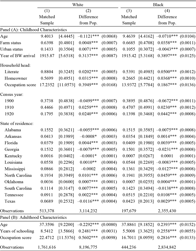
We show in Table 1 that men in the matched sample come from higher socioeconomic backgrounds on average than the population at risk to match, which is common in the matching literature (see, e.g., Abramitzky, Boustan, and Eriksson Reference Abramitzky, Boustan and Eriksson2012; Eriksson Reference Erikssonforthcoming). Specifically, childhood household heads of matched individuals are more likely to be literate, own their homes, and have higher occupational income scores, relative to those of the population.Footnote ²² Additionally, matched individuals themselves completed more years of schooling on average than the population. Because of this, we later weight linked individuals using inverse probability weights constructed so that the preferred matched sample is representative of the population on the variables shown in Table 1. Our results are not driven by differential selection into the matched sample.

Table 1

COMPARING THE MATCHED SAMPLE TO THE FULL POPULATION

+ = Significant at the 10 percent level.

* = Significant at the 5 percent level.

** = Significant at the 1 percent level.

*** = Significant at the 0.1 percent level.

Notes: The matched sample includes male children between the ages of 3 and 18 in 1900, 1910, and 1920, matched to adult educational outcomes in 1940. Columns (1) and (3) report means for the matched sample with standard deviations in brackets. Coefficients in Columns (2) and (4) are from regressions of individual characteristics of interest on an indicator for being in the matched sample. Thus, these columns show the difference between the matched sample and population with standard errors in parentheses.

Source: See the text.

The Boll Weevil, Enrollment, and Attendance

Baker (Reference Baker2015) showed that the boll weevil increased the enrollment rate of black children by 4 percent, and had a positive but not statistically significant effect on the white enrollment rate, in Georgia. In this section, we confirm that the boll weevil had a positive effect on enrollmentFootnote ²³ using county-level data from 1900 to 1934 for six Southern states of the Cotton Belt: Alabama, Arkansas, Georgia, North Carolina, South Carolina, and Tennessee.Footnote ²⁴ This yields a sample of 327 geographically consistent counties which were invaded by the boll weevil between 1906 and 1922.Footnote ²⁵

To begin, we estimate the effect of the boll weevil on enrollment using the following specification:

(1)$$In{(enrollment)_{ct}}{\rm{ }} = {\rm{ }}\beta boll{\rm{ }}weevi{l_{ct}} + \gamma In{(teachers)_{ct}} + {\theta _c}{\rm{ + }}{\theta _t} + {\phi _c}t + {\varepsilon _{ct}},$$

where boll weevil_ct is an indicator for the presence of the boll weevil which takes the value one if year t is greater than or equal to year of infestation in county c, and zero otherwise.Footnote ²⁶ Additionally, we include the natural log of the number of teachers, as a county-level control for school quality; county fixed effects $${\theta _c}$$ ; year fixed effects $${\theta _t}$$ ; and county-specific linear time trends $${\phi _c}t$$ . Equation (1), therefore, represents a difference-in-difference approach with identification of $$\beta $$ exploiting the differential timing of the year of infestation across counties. For example, the change in log enrollment, from before and after the boll weevil’s arrival, in newly infested counties is compared with the change in log enrollment over the same time period in as yet boll weevil–free counties, while controlling for unobserved county-level variables that remain fixed over time, to capture the level shift in log enrollment associated with the boll weevil infestation.

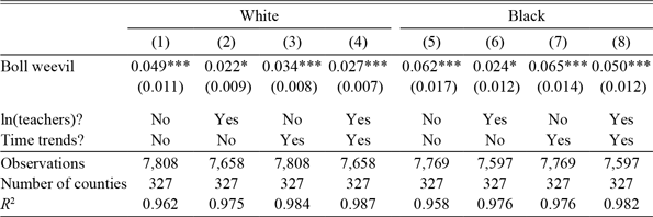
Table 2 presents the results. Columns (1) through (4) provide estimates for whites, while Columns (5) through (8) show estimates for blacks. The coefficients on the presence of the boll weevil indicator suggest the infestation had a positive and statistically significant effect on enrollment of both races. The coefficient in Column (4) of 0.027 suggests the boll weevil infestation led to a 2.7 percent ( $${e^{0.027}} - 1$$ ) increase in school enrollment of white children. That is an increase in enrollment of 107 white children in the average county. The coefficient in Column (8) of 0.050 suggests the boll weevil infestation led to a 5.1 percent increase in school enrollment of black children, an increase of 123 black children in the average county. The estimated coefficients for blacks are consistently higher than those for whites, and in specifications including county-specific linear time trends they are statistically different from one another at the 90 percent confidence level.

Table 2

ESTIMATES OF THE BOLL WEEVIL’S EFFECT ON LN(ENROLLMENT)

+ = Significant at the 10 percent level.

* = Significant at the 5 percent level.

** = Significant at the 1 percent level.

*** = Significant at the 0.1 percent level.

Notes: The dependent variable is the natural log of enrollment. Standard errors adjusted for clustering by county in parentheses. All regressions include year and county fixed effects. Columns (2), (4), (6), and (8) include the natural log of the number of teachers employed as a control for the supply of education. Columns (3), (4), (7), and (8) also include county-specific linear time trends.

Source: See the text.

To better understand the timing of the weevil’s effect on enrollment, we replace the boll weevil indicator with 6 leads and 12 lags for the year of the insect’s arrival. The specification becomes

(2) $$ln{\left( {enrollment} \right)_{ct}} = \mathop \sum \limits_{k \ge - 6,k \ne 0}^{k \le 12} {\beta _k}\ast 1\left\{ {t - B{W_c} = k} \right\} + \gamma ln{\left( {teachers} \right)_{ct}} + {\theta _c} + {\theta _t} + {\phi _c}t + {\varepsilon _{ct}}$$

where $$B{W_c}$$ represents the year of infestation of county c. Equation (2) also includes the natural log of the number of teachers (to control for the supply of education), county fixed effects, year fixed effects, and county-specific linear time trends. The indicator for the initial year of arrival is omitted; therefore, all effects are relative to the arrival date of the boll weevil. The coefficient $${\beta _{12}}$$ represents the average effect 12 or more years after being infested (relative to the year of arrival), while $${\beta _{ - 6}}$$ gives the effect six or more years before infestation.

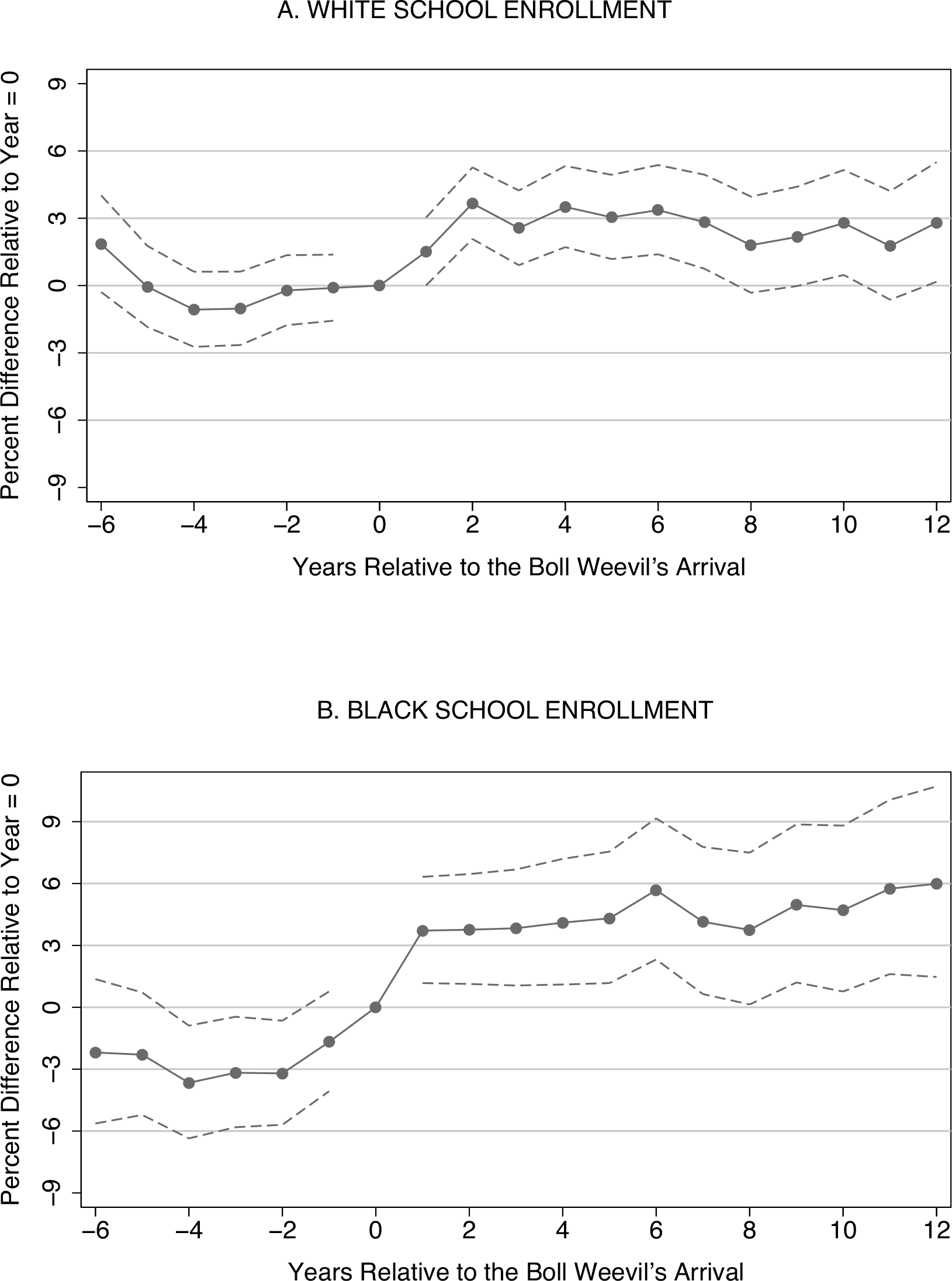
Figure 1 presents transformed coefficients of the leads and lags. Solid lines provide the main effects, while dashed lines represent 95 percent confidence intervals. Panel (A) shows school enrollment of whites remained fairly flat in the years leading up to the boll weevil’s arrival, with some decline in enrollment occurring six or more years prior to contact. Relative to the year of infestation, white enrollment had increased by approximately 3 percent two years later, with the estimated effect remaining near 3 percent up to 12 years later. Panel (B) shows the school enrollment of blacks was also relatively steady prior to the boll weevil, with an increase in enrollment occurring in the year of infestation. Three years after the arrival date, black enrollment had increased by approximately 4 percent compared to the year of infestation. These enrollment gains climb further to 6 percent and persist up to 12 years after the initial boll weevil infestation.

Figure 1

SCHOOL ENROLLMENT RELATIVE TO THE BOLL WEEVIL’S ARRIVAL

Notes: The y-axis shows the percent change in enrollment relative to the boll weevil’s year of arrival. The dashed lines indicate 95 percent confidence intervals.Source: See the text.

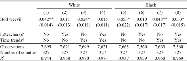
While the boll weevil had a positive effect on enrollment, it is unclear if this effect translated to higher attendance. In Table 3, we resolve this uncertainty by showing results of specifications replacing enrollment in Equation (1) with average daily attendance. The coefficient in Column (4) of 0.015 suggests the boll weevil infestation led to a 1.5 percent ( $${e^{0.015}} - 1$$ ) increase in school attendance of white children, yet this coefficient is not statistically significant at the 90 percent confidence level. Meanwhile, the coefficient of 0.033 in Column (8) suggests the boll weevil’s arrival led to a statistically significant 3.4 percent increase in school attendance of black children. Comparable coefficients across race are not statistically different from one another, even though the point estimates are higher for blacks.

Table 3

ESTIMATES OF THE BOLL WEEVIL’S EFFECT ON LN(ATTENDANCE)

+ = Significant at the 10 percent level.

* = Significant at the 5 percent level.

** = Significant at the 1 percent level.

*** = Significant at the 0.1 percent level.

Notes: The dependent variable is the natural log of average daily attendance. Standard errors adjusted for clustering by county in parentheses. All regressions include year and county fixed effects. Columns (2), (4), (6), and (8) include the natural log of the number of teachers employed as a control for the supply of education. Columns (3), (4), (7), and (8) also include county-specific linear time trends.

Source: See the text.

Unlike Baker (Reference Baker2015), who only finds a statistically significant response for blacks, we find statistically significant effects of the boll weevil on enrollment and attendance for both races when considering a broader set of states. The differences in our estimates are perhaps accounted for by heterogeneous responses to the boll weevil across states or greater precision due to the larger sample size.Footnote ²⁷ Nevertheless, many white children also worked in the cotton fields, so finding that the boll weevil had a positive effect on white enrollment is not particularly surprising. However, it should also be noted that our results are not directly comparable to those of Baker, as his dependent variable is enrollment rate while we consider enrollment without controlling for the school-age population.Footnote ²⁸

In fact, the results presented in this section must be interpreted with some degree of caution with respect to mechanisms, because we do not account for the school-age population. Boll weevil–driven in-migration prior to infestation and out-migration after infestation would both bias our estimates of the insect’s impact on enrollment toward zero, assuming that some migrants were enrolled in school. While the opposite, out-migration prior to infestation and in-migration after infestation, would bias our estimates upward. While we cannot rule out the possibility that our estimates are biased by boll weevil–induced migration, Lange, Olmstead, and Rhode (2009) show that population increased in advance of the boll weevil infestation, and declined afterward. This suggests that our estimates of the weevil’s impact on enrollment are biased toward zero, or conservative.Footnote ²⁹ Thus, they provide suggestive evidence that children, previously not in school, enrolled after the arrival of the boll weevil, or already enrolled children stayed in school longer than they would have in the absence of the boll weevil infestation.

While increased enrollment following the boll weevil’s arrival is suggestive of improved student outcomes, it does not directly follow that the weevil caused increased educational attainment, which is of much greater economic importance than school enrollment. Even if we were able to control for the school-age population, it would be necessary to assume that newly enrolled students were attending classes and completing grades to use the enrollment results to derive implications for educational attainment. As enrollment merely implies attendance for at least one day during the school term, these are not trivial assumptions. Indeed, the estimates showing average daily attendance was less responsive than enrollment to the boll weevil suggest that new enrollees had worse than average attendance records. It is certainly possible that the boll weevil increased enrollment while having little to no effect on grade completion, and thereby educational attainment. Therefore, we use our linked-census sample to directly investigate the weevil’s impact on years of schooling, in the next section.

Boll Weevil and Long-Run Schooling Outcomes

In our linked census data we follow individuals over time, but observe their years of schooling only in the 1940 census manuscripts, when they are adults. Therefore, we examine the boll weevil’s impact on educational attainment by comparing adjacent birth cohorts. Our main specification is a differences-in-differences approach where we compare those who were children (ages 4 through 18), and still eligible for public schooling, when the boll weevil arrived to older cohorts (ages 19 through 30), who likely completed their schooling prior to the infestation.Footnote ³⁰ This approach is represented by the following regression equation:

(3) $${y_{ica}} = \mathop \sum \limits_{k = 0}^4 {\beta _k}\ast 1\left\{ {3\left( {5 - k} \right) + 1 \le B{W_c} - a \le 3\left( {6 - k} \right)} \right\} + \gamma {X_i} + {\theta _c} + {\theta _a} + {\varepsilon _{ica}}$$

where $${y_{ica}}$$ is an educational outcome of interest for individual i, who was born in year a and observed in county c in childhood (between the ages of 3 and 18, inclusive).Footnote ³¹ Boll weevil exposure occurs at age $$B{W_c} - a$$ , where BW_c represents the year of infestation of county c.Footnote ³² Therefore, the indicator function ( $$1\left\{ {3\left( {5 - k} \right) + 1 \le B{W_c} - a \le 3\left( {6 - k} \right)} \right\}$$ ) returns a one if the individual was aged 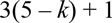$$3\left( {5 - k} \right) + 1$$ through $$3\left( {6 - k} \right)$$ in the year of infestation, and zero otherwise. The $${\theta _c}$$ and $${\theta _a}$$ are county and birth cohort fixed effects, respectively, while $${X_i}$$ is a vector of individual-level family background controls as measured in the childhood census year. Family background controls include childhood household head’s occupational income score, homeownership status, and literacy, as well as indicators for urban location and farm residence. The $${\beta _k}$$ are the coefficients of interest, representing the average treatment effect of the boll weevil on individuals in the relevant exposure cohort. Because the boll weevil arrived at different times in different counties we are able to separately identify the full set of birth cohort and county fixed effects as well as the treatment effects for those exposed at age 18 or under.

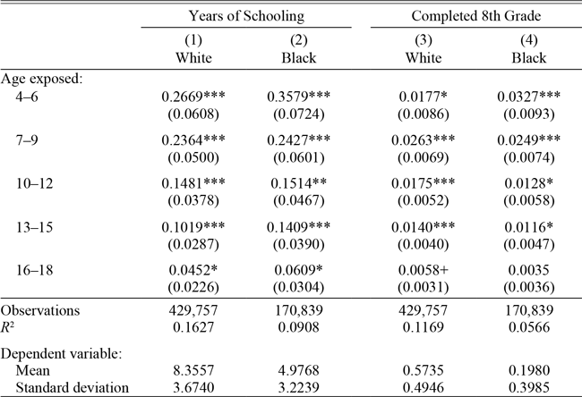
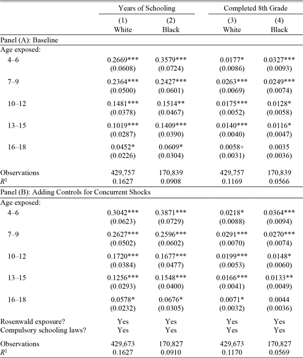
The first two columns of Table 4 show the results of regressions following Equation (3) with years of schooling as the dependent variable. Children who were first exposed to the boll weevil between the ages of 4 and 6, inclusive, saw the greatest gains in years of schooling as a result. White children exposed at ages 4–6 attained 0.2669 more years of schooling on average, as compared with those exposed at ages 19–30 (shown in Column [1]). White children exposed at 7–9 years of age experienced similar relative gains of 0.2364 years of schooling. Both results are statistically significant at the 99.9 percent confidence level. Whites exposed to the boll weevil at older ages of 10–12 and 13–15 saw smaller increases in educational attainment of 0.1481 and 0.1019 years of schooling, respectively. If the opportunity cost of schooling is increasing in years of schooling and work experience, and the timing of the transition from schooling to working maximizes expected present value of lifetime earnings, then a modest negative shock to the opportunity cost of schooling will induce those in school to stay in school longer but will affect few who have already left school for work.Footnote ³³ Thus, not surprisingly, whites exposed to the boll weevil between the ages of 16 and 18 saw an increase in educational attainment of only 0.0452 years on average, relative to those exposed at ages 19–30, and this result is statistically different from zero only at the 95 percent confidence level. Column (2) shows remarkably similar gains in educational attainment for blacks resulting from the boll weevil infestation. The only coefficient that differs notably, but not statistically, from those of whites is that for the youngest exposure cohort; black children exposed at ages 4–6 attained 0.3579 more years of schooling on average, compared to those exposed at ages 19–30.

Table 4

ESTIMATES OF THE BOLL WEEVIL’S EFFECT ON LONG-RUN EDUCATIONAL OUTCOMES

+ = Significant at the 10 percent level.

* = Significant at the 5 percent level.

** = Significant at the 1 percent level.

*** = Significant at the 0.1 percent level.

Notes: The dependent variables are given in the column headings. Standard errors adjusted for clustering by childhood county of residence are in parentheses. All specifications include year of birth fixed effects, childhood county of residence fixed effects, and controls for family background. Family background controls include childhood household head’s occupational score, homeownership status, and literacy, as well as indicators for urban location and farm residence.

Source: See the text.

Columns (3) and (4) of Table 4 instead consider the boll weevil’s impact on eighth grade completion.Footnote ³⁴ Again, children exposed to the boll weevil at younger ages were more responsive in their likelihood of completing at least eight years of schooling. As shown in Column (3), white children exposed at ages 7–9 were more likely to complete the eighth grade by 2.63 percentage points, compared with those exposed at ages 19–30. Black children saw a similar increase, of 2.49 percentage points, in the likelihood of graduating grammar school due to boll weevil exposure at ages 7–9, as indicated in Column (4). Differences in point estimates are not statistically significant across race and are generally quite small.

In interpreting the $${\beta _k}$$ as average treatment effects, we are implicitly making the assumption that individuals between the ages of 19 and 30 when the boll weevil arrives in their childhood county of residence do not alter their years of schooling or grade completion rates in response. Indeed, there are structural reasons to expect 19 to 30 year olds to be little affected by the weevil; children generally attend school, while adults generally work. When the outcome of interest is eighth grade completion, this seems like a quite reasonable assumption as the typical age for finishing eighth grade is 14. While age-for-grade statistics were not commonly published by Southern states during the early twentieth century, a report on the 1923 school year in Tennessee reveals that approximately 1.3 percent of whites and 3.3 percent of blacks ages 19–21 were enrolled in grades one through eight (Tennessee Department of Education 1924). Thus, the boll weevil is unlikely to have had a discernible impact on eighth grade completion for exposure cohorts over the age of 19. However, with years of schooling as the outcome, the validity of this assumption is not as clear. The 1920 census shows that 4.3 (2.2) percent of white (black) Southern-born men ages 19–30 were still attending school.Footnote ³⁵ If the boll weevil had a positive (negative) effect on the educational attainment of individuals in older exposure cohorts, then the coefficients shown in Table 4 may understate (overstate) the true effects. Therefore, we next consider the possibility of pre-trends (or the validity of 19–30 year old exposure cohorts as a comparison group).Footnote ³⁶

It is common for studies taking an empirical approach of the form specified in Equation (3) to also show results of a regression equation with both leads and lags on treatment, to allay concerns regarding the possibility of preexisting trends, like the following:

(4) $${y_{ica}} = \mathop \sum \limits_{k \ge - 4,k \ne - 1}^{k \le 4} {\beta _k}\ast 1\left\{ {3\left( {5 - k} \right) + 1 \le B{W_c} - a \le 3\left( {6 - k} \right)} \right\} + \gamma {X_i} + {\theta _c} + {\theta _a} + {\varepsilon _{ica}}$$

Such results are often shown graphically. However, Borusyak and Jaravel (Reference Borusyak and Jaravel2017) point out the results of such a regression are underidentified due to the absence of a truly untreated control group. In our case, it is not possible to fully disentangle the birth cohort effects $${\theta _a}$$ from exposure cohort effects $${\beta _k}$$ in the presence of county fixed effects $${\theta _c}$$ . The simplest solution to this underidentification problem would be to drop the county fixed effects. However, county fixed effects are necessary for identification since the timing of the boll weevil’s arrival is not independent of time invariant county characteristics (e.g., longitude, latitude, and climate).Footnote ³⁷

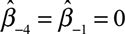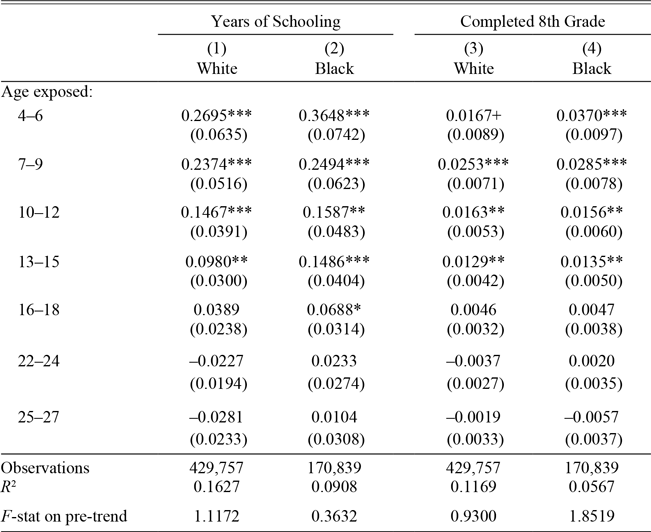
Instead, we follow the recommendation of Borusyak and Jaravel (Reference Borusyak and Jaravel2017), imposing the restrictions that $${\widehat\beta _{ - 4}} = {\widehat\beta _{ - 1}} = 0$$ . In practice, this means dropping two indicators for older exposure cohorts: those exposed at 19–21 and 28–30. Then, an F-test on the joint significance of the remaining pre-trends provides a test for the existence of non-linear pre-trends. Given the nonlinearity in attendance rates between 19–21 year olds and older age groups, we would expect to see evidence of non-linear pre-trends if those exposed at 19–21 were modifying their schooling behavior in response to the boll weevil. The results of these restricted regressions are shown in Table 5.Footnote ³⁸ The fact that the coefficients on the 4–6 to 16–18 exposure cohort indicators are little affected, compared to those presented in Table 4, is encouraging. The coefficients on the indicators for exposure to the boll weevil at ages 22–24 and 25–27 are small in magnitude and not statistically different from zero. Moreover, the F-statistics on their joint significance are below 2.31, the critical value of F for the $$\alpha = 0.1$$ significance level, so we cannot reject the null hypothesis that the coefficients on the remaining pre-trends jointly equal zero. This provides reasonable reassurance against the presence of non-linear pre-trends, as would be likely if older exposure cohorts modified their schooling behavior due to, or in anticipation of, the boll weevil’s arrival.Footnote ³⁹

Table 5

THE BOLL WEEVIL’S EFFECT ON LONG-RUN EDUCATIONAL OUTCOMES WITH PRE-TRENDS

+ = Significant at the 10 percent level.

* = Significant at the 5 percent level.

** = Significant at the 1 percent level.

*** = Significant at the 0.1 percent level.

Notes: The dependent variables are given in the column headings. Standard errors adjusted for clustering by childhood county of residence are in parentheses. All specifications include year of birth fixed effects, childhood county of residence fixed effects, and controls for family background. Family background controls include childhood household head’s occupational score, homeownership status, and literacy, as well as indicators for urban location and farm residence.

Source: See the text.

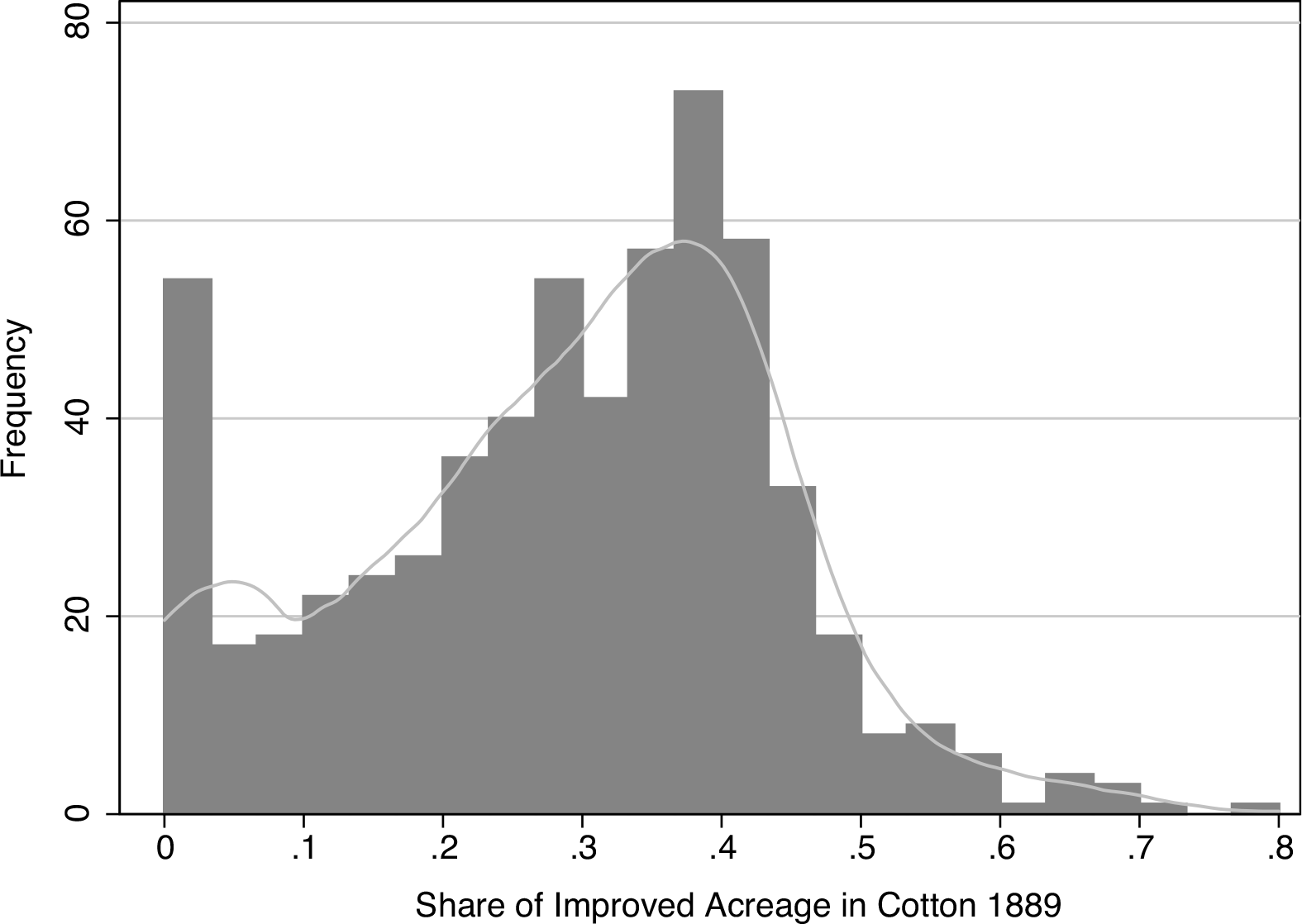
We also investigate whether the boll weevil’s effect on years of schooling differed according to the intensity of cotton production in one’s childhood county of residence. We use the ratio of acres in cotton to improved farm acreage in 1889 as a measure of cotton intensity prior to the boll weevil’s arrival.Footnote ⁴⁰ Figure 2 reveals, for our linked sample, the county-level distribution of the share of improved acreage planted in cotton in 1889. The median county in our sample grew cotton on 30.4 percent of improved acreage, while the 95th percentile was 50.6 percent.

Figure 2

DISTRIBUTION OF SAMPLE COUNTIES BY INTENSITY OF COTTON PRODUCTION

Notes: Cotton intensity is defined as the ratio of acres planted in cotton to improved farm acreage as measured in 1889. The solid line provides the kernel density estimate of the distribution.Source: Haines and ICPSR (2010).

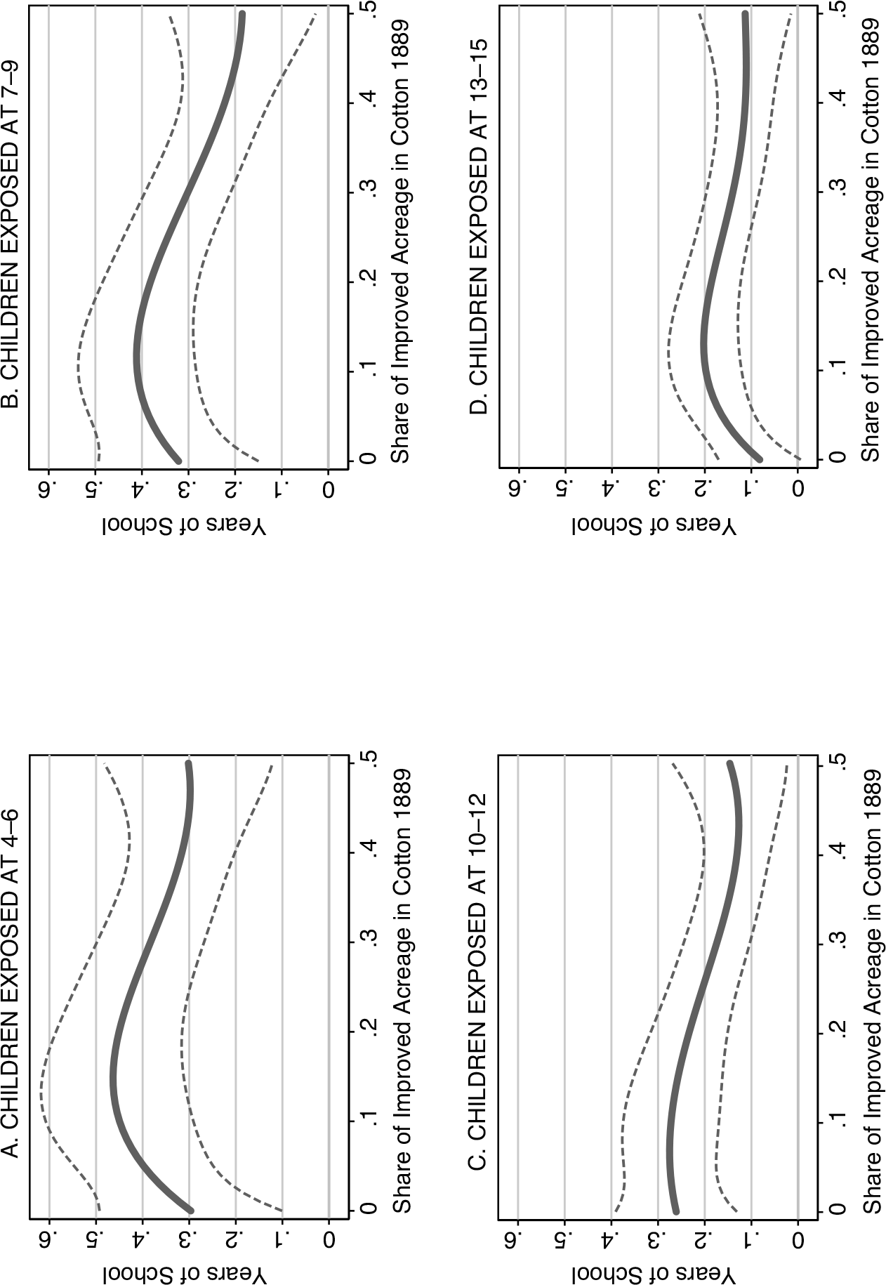
We modify Equation (3) by interacting each exposure cohort indicator with a 4th-order polynomial in cotton intensity.Footnote ⁴¹ Figure 3 reveals the predicted impact of exposure to the boll weevil at ages 4–6 (Panel [A]), 7–9 (Panel [B]), 10–12 (Panel [C]), and 13–15 (Panel [D]) on years of schooling as it varies by cotton intensity in childhood county of residence.Footnote ⁴² Figure 3 shows substantial positive effects on educational attainment, even in counties with little cotton production in 1889. The boll weevil’s effect on years of schooling increases further as intensity of cotton production rises to approximately 15 percent. The youngest exposure cohort (4–6 year olds in Panel [A]) experienced a 0.15 year increase in schooling as cotton acreage went from 0 to 15 percent, that is a 50 percent increase in the estimated effect relative to those in counties with no cotton acreage. Then, the impact of the weevil declines from its peak as cotton intensity increases from 15 to 50 percent of farm acreage. Panel (A) shows that the decline for the youngest exposure cohort mirrors the rise, falling by approximately 0.15 years of schooling. However, the 7–9 (Panel [B]) and 10–12 (Panel [C]) exposure cohorts saw larger declines relative to the preceding rise. For example, point estimates for the 7–9 exposure cohort suggest gains in educational attainment of 0.32 years in counties with little cotton acreage, 0.40 years in counties with 15 percent of acreage in cotton, and 0.18 in counties with 50 percent of improved land in cotton.

Figure 3

IMPACT OF THE BOLL WEEVIL ON YEARS OF SCHOOLING BY INTENSITY OF COTTON FARMING IN 1889

Source: See the text.Notes: The y-axis shows the difference in years of schooling relative to individuals exposed to the boll weevil between the ages of 19 and 30, inclusive. The dashed lines indicate 95 percent confidence intervals. Adjusted R2 = 0.2038.

The predicted effects by cotton intensity suggest that children in counties where cotton production was marginally optimal benefited the most from the weevil with respect to educational attainment, while children in counties that were heavily dependent on cotton cultivation benefited to a lesser extent. At first glance, this might seem counterintuitive. However, bear in mind that these estimates reflect the overall impact of the boll weevil on educational attainment; the expected gains in attainment resulting from the decline in the opportunity cost of schooling, due to substitution away from cotton, are partially offset by an increased desire for children to generate earnings as a result of the weevil’s negative effect on household income. Therefore, the estimated effects shown in Figure 3 would be expected if the propensity to switch crops after infestation decreased, or the magnitude of the income shock due to the weevil increased, with cotton intensity. Indeed, empirical and anecdotal evidence suggests that the boll weevil did greater damage where cotton was more intensely grown and substitution away from cotton, in terms of acreage, was greatest where the crop was marginally optimal (Giesen Reference Giesen2011; Lange, Olmstead, and Rhode 2009). The estimates presented in Figure 3, then, are consistent with expectations that education gains were most pronounced in locations where substitution away from cotton was greatest and income effects were limited; while counties where the boll weevil had large negative effects on income, and yet substitution away from cotton was relatively limited, saw more modest gains in educational attainment.

There is also a possibility that migration plays a role in generating the patterns observed in Figure 3. Lange, Olmstead, and Rhode (2009) show that counties with high levels of cotton intensity, relative to those with moderate levels, experienced greater declines in population, by approximately a factor of two, following the boll weevil’s arrival. They suggest these population declines could be explained by migration from infested counties to cotton counties not yet affected by the boll weevil. If this accurately describes the pattern of migration, then a larger share of children whom we observe in high-cotton-intensity counties, relative to children observed in moderate-cotton-intensity counties, would have moved just after the weevil’s arrival to boll weevil–free cotton-producing counties. These children would not have experienced a reduction in the opportunity cost of schooling generated by substitution away from cotton to alternatives less suited to child labor, as would the non-migrant population, and thus we would not expect to see gains in educational attainment due to boll weevil exposure for these children. Therefore, the estimated effect of the boll weevil on the educational attainment of children located in high-cotton-intensity counties before infestation could be lower than in moderate-cotton-intensity counties, even if the weevil’s effect among the non-migrant population was constant in cotton intensity. Alternatively, it is possible that these children migrated, instead, to urban areas, or the North, which would have provided improved educational opportunities. Regardless, boll-weevil induced migration should not be interpreted as biasing our results since our goal is to quantify the overall effect of the weevil on educational attainment, inclusive of effects running through the migration channel.

Concurrent Shocks to Education

A possible threat to validity regards shocks to educational resources and requirements contemporaneous with the weevil infestation. Events that overlapped in timing with the boll weevil’s spread and significantly affected educational attainment include the passage of compulsory school attendance laws (Lleras-Muney Reference Lleras-Muney2002) and the construction of Rosenwald schools (Aaronson and Mazumder Reference Aaronson and Mazumder2011). If the passage of compulsory schooling laws or Rosenwald school construction were correlated with the onset of the boll weevil infestation, this could result in spurious correlation between boll weevil exposure and student outcomes.

Therefore, we assign to individuals in our sample a measure of Rosenwald school exposure, based on childhood county of residence and year of birth, and include this and its interaction with an indicator for rural status as controls. Additionally, we calculate the number of years of schooling required, by state and birth cohort, from the ages for which compulsory schooling laws required attendance and the effective dates of those laws, adding this measure as a control.Footnote ⁴³ Panel (B) of Table 6 shows the results of our main specifications modified to add controls for compulsory schooling and Rosenwald school exposure. The coefficients presented are comparable in magnitude, if not slightly larger, and statistical significance to the baseline results, which are repeated in Panel (A) for convenience, ameliorating concern that omitted variable bias is driving our results.

Table 6

ROBUSTNESS OF THE BOLL WEEVIL’S EFFECT ON EDUCATIONAL OUTCOMES TO CONCURRENT SHOCKS

+ = Significant at the 10 percent level.

* = Significant at the 5 percent level.

** = Significant at the 1 percent level.

*** = Significant at the 0.1 percent level.

Notes: The dependent variables are given in the column headings. Standard errors adjusted for clustering by childhood county of residence are in parentheses. All specifications include year of birth fixed effects, childhood county of residence fixed effects, and controls for family background. Family background controls include childhood household head’s occupational score, homeownership status, and literacy, as well as indicators for urban location and farm residence. Additionally, specifications in Panel (B) include a measure of Rosenwald school exposure, its interaction with an indicator for rural status, and a measure of exposure to compulsory school attendance laws as controls for contemporaneous shocks to education.

Source: See the text.

Robustness to Matching

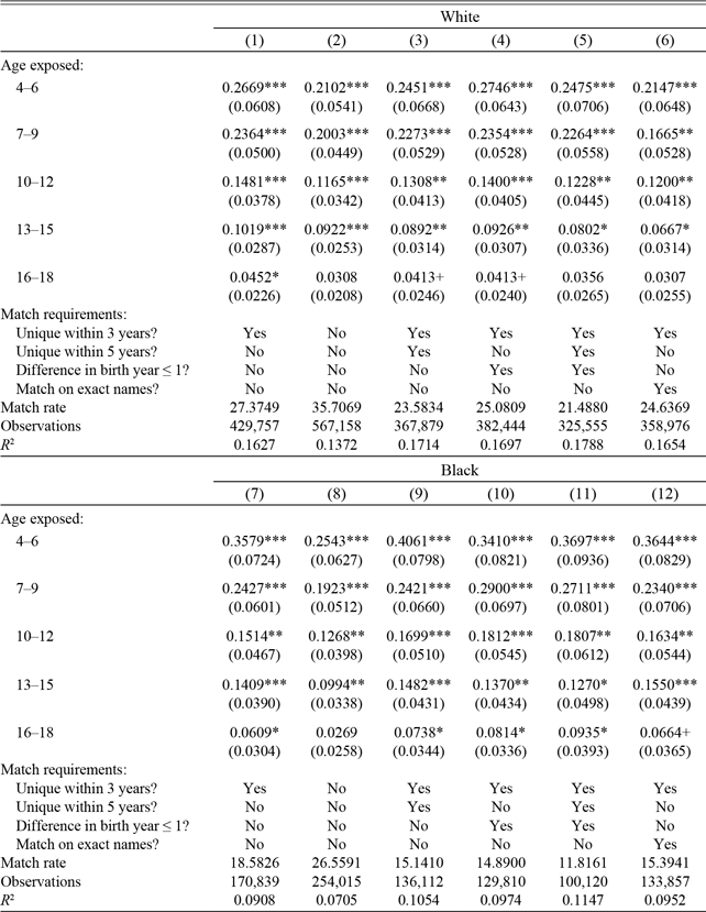
Table 7 presents results of specifications, following Equation (3) with years of schooling as the dependent variable, utilizing samples generated by several different matching procedures. Columns (1) through (6) show results for whites, while Columns (7) through (12) display results for blacks. The first columns for each race, (1) and (7), reproduce results utilizing our baseline sample, those shown in Table 4, for ease of comparison. Columns (2) and (8) relax match restrictions slightly by allowing matches between individuals that are not unique within three-year age bands. The methodology in this sample is, therefore, identical to Abramitzky, Boustan, and Eriksson (Reference Abramitzky, Boustan and Eriksson2012). This method results in a match rate of 35.71 (26.56) percent for the white (black) sample, significantly higher than the 27.37 (18.58) percent match rate of the baseline. Relaxing restrictions yields point estimates that are smaller in magnitude by 15 to 29 percent relative to the baseline for the youngest three exposure cohorts, but still statistically significant. This is likely due to attenuating noise introduced by a higher level of false positive matches.

Table 7

ROBUSTNESS OF THE BOLL WEEVIL’S EFFECT ON YEARS OF SCHOOLING TO MATCHING

+ = Significant at the 10 percent level.

* = Significant at the 5 percent level.

** = Significant at the 1 percent level.

*** = Significant at the 0.1 percent level.

Notes: The dependent variable is years of schooling. Standard errors adjusted for clustering by childhood county of residence are in parentheses. All specifications include year of birth fixed effects, childhood county of residence fixed effects, and controls for family background. Family background controls include childhood household head’s occupational score, homeownership status, and literacy, as well as indicators for urban location and farm residence. Columns (1) and (7) repeat the baseline results shown in Table 4 for ease of comparison. Match rates are calculated relative to the 1940 population of men between the ages of 23 and 58, inclusive, with recorded level of education.

Source: See the text.

Matching restrictions are increased relative to the baseline, to further reduce the likelihood of false positive matches, in Columns (3) and (9), which require individuals to be unique within five-year age bands. The match rate falls to 23.58 (15.14) percent for the white (black) sample, yet the coefficients are not meaningfully changed compared with the baseline. Columns (4) and (10) show results from a matched sample requiring that individuals be unique within three-year age bands and have absolute differences in year of birth of less than or equal to one year. The latter restriction is also aimed at reducing the frequency of false positive matches, as those with two-year discrepancies in year of birth are more likely to be incorrect. Again, the coefficients are remarkably similar to the baseline. Columns (5) and (11) additionally restrict matches to individuals that are unique within five-year age bands, and present results that are nearly identical. Columns (6) and (12) return to the three-year age band uniqueness restriction, but require matches on exact names rather than standardized versions of names. Results are little changed for blacks here, but point estimates are reduced in magnitude for whites by 19 to 30 percent relative to the baseline for the youngest three exposure cohorts.Footnote ⁴⁴

Robustness to Weighting

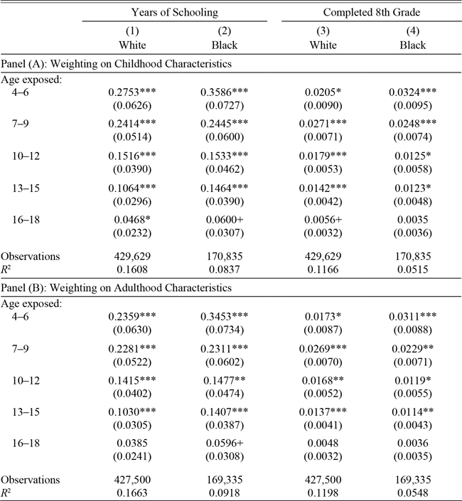
Recall that the baseline sample is not representative of the population, as shown in Table 1. In Table 8, we examine whether the results are robust to weighting the baseline sample to be representative of the population along the characteristics presented in Table 1. Panel (A) presents specifications analogous to the baseline shown in Table 4, but uses inverse probability weights calculated based on family background characteristics provided by childhood census data. Instead, Panel (B) uses inverse probability weights estimated from 1940 census characteristics. The results presented do not meaningfully differ from the baseline results. Therefore, our results cannot be explained by observable differences between the population and the matched sample.

Table 8

ROBUSTNESS OF THE BOLL WEEVIL’S EFFECT ON LONG-RUN EDUCATIONAL OUTCOMES TO WEIGHTING

Notes: The dependent variables are given in the column headings. Standard errors adjusted for clustering by childhood county of residence are in parentheses. All specifications include year of birth fixed effects, childhood county of residence fixed effects, and controls for family background. Family background controls include childhood household head’s occupational score, homeownership status, and literacy, as well as indicators for urban location and farm residence. The specifications in Panel (A) use an inverse proportional weighting method to weight our matched sample to be reflective of the population with respect to observable childhood characteristics: census year; state of residence; race; age; household head’s occupational score, homeownership, and literacy; household farm and urban status; and year of infestation of county of residence. The specifications in Panel (B) use an inverse proportional weighting method to weight our matched sample to be reflective of the population with respect to observable adulthood characteristics: state of residence; race; age; years of schooling; and occupational income score.

Source: See the text.

+ = Significant at the 10 percent level.

* = Significant at the 5 percent level.

** = Significant at the 1 percent level.

*** = Significant at the 0.1 percent level.