The Solow growth and the Heckscher-Ohlin trade models describe two competing processes through which regional incomes converge over time. Solow's model attributes rising productivity of labor to additional regional capital investments. Heckscher-Ohlin's trade model ascribes the relocation of high value industries to regions with low wage rates. On the other hand Paul Krugman expects incomes to diverge over time as regions with an initial advantage maintain it through ever increasing external economies of scale. The Solow and Heckscher-Ohlin models imply that incomes converge through the movement of high quality labor and capital and high value goods and services into low income regions respectively.
In 1951 Frank Hanna recognized that an index of average income per worker of a region compared to the same average for the nation equals the sum of the region's wage and industry effects.1
Hanna, “Contribution,” pp. 18–19.
A Hanna wage index compares the sum of average wage per worker per sector between the region and the nation weighted by the relative importance of the sectors in the region. The Hanna industry index compares the sum of the relative importance of each sector between the region and the nation weighted by the average wage per worker per sector for the nation. The industry index measures the effect on average wages from some sectors consistently paying higher wages than others. For example, the aggregate “nonagricultural sector” pays higher wages than the agricultural sector. Ceterus paribus, a region with a larger portion of its economy devoted to the nonagricultural sector will have relatively higher average income.
In 1998 Sukkoo Kim applied Hanna's income index to measuring the relative importance of the wage and industry effects. In particular, he measured the contribution of these effects for each of nine census regions of the United States at five points in time between 1840 and 1987. If the Solow theory were right, Kim would find no industry effect and decreasing wage effects over time. If the Heckscher-Ohlin theory were right, he should observe the opposite. Were the Hanna indices more consistent with those predicted by the Solow or the Heckscher-Ohlin theory?
From this research, Kim drew six conclusions about the convergence of wages across the regions of the United States. In a note, Sumner La Croix used Kim's data and applied his own index number approach. La Croix's wage and industry indices resulted in some contradictions to those developed by Kim using the Hanna index approach. More importantly, La Croix's results cast doubt on three of the six conclusions stated by Kim.
La Croix and Kim both accepted the following three conclusions: First, “the most significant cause of income divergence between 1840 and 1900 was the sharp relative decline in Southern income per capita caused by the region's growing unfavorable industry mix and lower wages relative to other regions.”2
Kim, “Economic Integration,” p. 672.
Second, “for all regions in 1954 the income differences that can be attributed to the industry-mix effects were considerably lower than they were in 1900.”
3 Kim, “Economic Integration,” p. 677.
Third, “the favorable industry-mix income effect for the New England and Middle Atlantic regions fell from 25 percent to less than 10 percent between 1900 and 1954.”
4 Kim, “Economic Integration,” p. 677.
However, three statements by Kim differed from La Croix's results. Kim concluded: “… for some regions, such as the New England and Middle Atlantic regions, favorable regional industrial structures were responsible for their relatively high aggregate income per capita. For other regions, such as the Mountain and Pacific regions, their relatively high aggregate incomes were attributed to favorable wages.”5
Kim, “Economic Integration,” pp. 671–72.
La Croix found that “The wages and industry-mix decompositions for the Middle Atlantic region in 1880 produced completely different results. Kim's industry-mix decomposition shows that 66.6 percent of the income differential for the Middle Atlantic regions is due to favorable industry mix.” The La Croix industry decomposition shows 33 percent due to industry mix in the region at that time.
6 La Croix, “Economic Integration,” pp. 777–78.
Second, Kim states: “… lower relative wages were more important than unfavorable industry-mix in explaining the relative decline in the income per capita of the South Atlantic and East South Central regions” in 1880 and 1900.7
Kim, “Economic Integration, p. 672.
La Croix on the other hand found that “… unfavorable industry mix explains a larger percentage of the East South Central region's income differential in 1880 and 1900 than lower relative wages.”
8 La Croix, “Economic Integration, p. 778.
Finally, Kim concludes: “… by 1987 differences in regional industrial structure accounted for only a small fraction of the differences in earnings.”9
Kim, “Economic Integration, p. 677.
La Croix states that: “… the average absolute value of the industrial mix differential falls from over 11 percent in both decompositions [in 1840] to 2.5 percent in Kim's decomposition and 2.7 percent in La Croix's decomposition [in 1987].”
10 La Croix, “Economic Integration, p. 778.
At the end of their exchange of notes, Kim and La Croix agreed that the Hanna and La Croix wage and industry indices sometime give “drastically different results.”11
Kim, “Decomposing,” pp. 780–81.
However, Kim minimized the importance of the problem by pointing out that 84 percent of the time there is 10 percent or less difference in the absolute values of the indices.
12 Kim, “Decomposing,” p. 783.
He also pragmatically suggests using both techniques and drawing conclusions only when both indices support an assertion.
13 Kim, “Decomposing,” p. 781.
In the end, however, he declares that “it is beyond the scope of this reply to suggest reasons why the decomposition procedure is not unique.”
14 Kim, “Decomposing,” p. 781.
My note takes up Kim's challenge to develop an approach that both resolves the Hanna and La Croix index inconsistency problem and explains why it happens.
THEORY
I start with a review of the original Hanna and La Croix income indices. Then a second-order Taylor series expansion of an assumed quadratic income function is used to derive the exact measures of wage and industry effects. I show that a second-order approximation of a constant elasticity of substitution (CES) function provides exact measures of wage and, by residual, industry effects as well. This leads to an illustration of W. E. Diewert's idea that the second-order wage index equals the geometric mean of two first-order approximations of a CES function. That result is used to prove that the original Hanna and La Croix indices are first-order approximations of an assumed Leontief income function. An explanation follows of why the geometric mean of the original Hanna and La Croix wage indices only approximates the CES wage index. Finally, a CES income index that measures each sector's contribution to the overall wage and industry effects is developed.
Let i equal the set of standard industrial classifications for the sectors in the economy, where, for example, i equals one and two for agriculture and nonagriculture sectors; j is the set of geographic regions of the United States where j equals zero to nine such that zero is the United States and one is the first region within the nation. Ej is the average income per job in region j. Wij is the average wage per job in sector i in region j. Nij is the employment in sector i in region j. sij is the share of jobs in sector i in region j. Sij is the share of wages in sector i in region j. μij is the industry mix coefficient in sector i in region j.
THE ORIGINAL HANNA AND LA CROIX WAGE AND INDUSTRY INDICES
Conceptually Hanna's original income decomposition equation is
15 Hanna, “Contribution,” p. 19.
This equation is calculated in natural logs as:
The income index E1/E0 is the ratio of the region's overall average income per job compared to that for the United States.
The Hanna wage index is
. This index compares wages between the region and the nation while holding industry mix constant and equal to the region's (si1). Hanna's interpretation of his wage index is “the differences in production-workers hourly earnings associated with differences among states in the wages paid production-workers in the same industry.”16
Hanna, “Contribution,” p. 18.
A wage index is one measure of the relative importance of Solow's growth theory to explain income convergence.
The Hanna industry index is
. This index compares industry mix of the region and the nation. For this comparison wages are held constant at the national average for each sector (Wi0). Hanna's definition of industry mix is “the differences among states' production-worker hourly earnings which is associated with differences in the composition of the state's manufacturing activities.”17
Hanna, “Contribution,” p. 18.
Kim defines the Hanna's industry index as “… based on the assumption that regions have different industrial structures but identical income per capita at the industry level. The industry income per capita for all regions is set equal to the national industry income per capita…. The difference between the two hypothetical incomes—industry-mix income and the overall national income—provides a measure of the income difference due to the divergence in regional industrial structure.”
18 Kim, “Economic Integration,” p. 671.
The original La Croix income decomposition is
19 La Croix, “Economic Integration,” p. 774.
The natural log of La Croix's equation used in the calculations is:
La Croix's wage index is
. This wage index is similar to Hanna's except the industry mix or share of jobs by sector for the region is assumed to equal that of the nation (si0). La Croix defines his wage index as “… income per capita under the assumption that regions have different per capita wage rates but identical industry-mixes. In the ‘wages’ decomposition, the industry-mix for all regions is set equal to the national industry-mix.”20
La Croix, “Economic Integration,” p. 774.
La Croix's industry index is
. The industry index is also similar to Hanna's except the wages for the nation are assumed to equal that of the region (Wi1). La Croix's interpretation of the industry mix index as the difference between the actual earnings per job and the hypothetical wages-variable income now provides a measure of the income differences due to differences in regional industry mix.21
La Croix, “Economic Integration,” p. 774.
The sum of wage and industry indices in their respective Hanna and La Croix equations equals the income index.
However neither the Hanna and La Croix wage nor the industry indices equals the other.
La Croix pointed out the difference between these indices could be so great as to lead to contradictory results, which makes reaching a conclusion impossible in some cases. An income index is needed that reconciles and explains theses differences.
TRANSFORMING THE HANNA AND LA CROIX INDICES
The La Croix income decomposition can be rewritten as:
where μ is the industry index. If we assume that μ=0, then equation 11 can be transformed into the following expression:
The transformed La Croix income index is
A similar transformation can be applied to the Hanna income index such that
We will return to these indices after we discuss the Taylor series approach for determining an exact income index.
A CES INCOME INDEX
Consider a quadratic income function that is continuous, linearly homothetic, nondecreasing, and convex in sector wages and subject to discrete changes in industry mix.
We know from calculus that it is possible to find the distance between two points on a continuous function with increasing accuracy using a Taylor series expansion. Taylor's Theorem: Let f be a function that is continuous together with its first n+1 derivatives on an interval containing a and x. Then the value of the function at x is given by
22 Thomas, “Calculus,” pp. 790–91.
Taylor's theorem states that it is possible to estimate any point on a continuous function as the sum of another point on the function (zero order), a tangent to the function at that point (first order), a quadratic approximation at that point (second order), and so on until the function is completely specified. Therefore the assumed quadratic income function needs a second-order approximation to be completely specified. Conversely it is not possible to exactly estimate a second-order function with a single first-order approximation. However, as we shall see later, it is possible to determine the second-order measure as the geometric mean of two first-order approximations.
We are interested in accurately measuring the difference between regional and national incomes E1 and E0 using only information about the average wages paid in each sector of each region (Wij) while assuming the industry mix is constant. In general a second-order Taylor series expansion of the quadratic income function is:
Hotelling has shown that the first derivative of a translog function with respect to price equals its factor share.
23 Hotelling, “Demand Functions,” pp. 71–74.
A logarithmic income function is one in which
f(
Wj)=ln
Ej and
Wij=ln
Wij. By applying Hotelling's lemma to the income function, we know that the first derivative of the function with respect to wages equals the wage share in each sector
i within the region.
A second derivative is the first derivative of a first derivative
Finally, Diewert's quadratic lemma states that the geometric mean of the first derivatives taken at both the initial and subsequent points on a quadratic function provides a second-order approximation of that function.
24 Diewert, “Exact,” p. 118.
Therefore, we can use either equation 19 or Diewert's lemma to derive the exact measure of the income index. If we use equation 19 the quadratic earning function is as follows.
The CES income index is
Where ln (1+μ) is the CES industry index and
is the CES wage index.
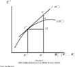
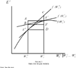
Alternatively, if we use Diewert's lemma, we begin by calculating two first-order approximations of the income function. The first is over the interval zero and one, and the second is the reverse. These intervals imply that we can assign the reference point to either the region or the nation when measuring the relative difference in income between them. This is the basis of the difference between the Hanna and La Croix approaches. A first-order Taylor series expansion of the income function Ej is estimated initially on the interval from zero to one. The result is a “Cobb-Douglas” Hanna income index. This index is based on the assumption that the underlying income function has the characteristics of a Cobb-Douglas function. In Figure 1 the Hanna wage index equals AB. We then reverse the interval and estimate the first order approximation over the interval from one to zero. The result is a Cobb-Douglas La Croix income index, CD in Figure 2.
These income functions are initially assumed to be Cobb-Douglas in nature. As such they have the characteristics of decreasing marginal rates of technical substitution of labor between sectors and unitarily elastic wage shares. If the income functions were Cobb-Douglas, then a first-order Taylor series approximation would accurately estimate it. This is because there is no change in wage shares so its second-order effects are zero. Since wage share in a Cobb-Douglas income function are fixed by definition, then Si1 equals Si0 and the wage indices would be equal. This result is a test of the assumption that the underlying income function is Cobb-Douglas in form.
The Cobb-Douglas Hanna Income Index is
The Cobb-Douglas La Croix Income Index is
If the wage shares are different we can assume the underlying income function is CES in form. A CES function is similar to a Cobb-Douglas function except the wage share changes due to constant but not unitary elasticity of substitution of labor. Diewert's lemma states that the average of two first-order approximations of a CES function equals its second-order or exact measure. Therefore the average of equations 21 and 22 equals equation 20. In Figure 3 the CES wage index is measured as 1/2(AB+CD).
RELATING THE ORIGINAL HANNA AND LA CROIX INDICES TO A CES INDEX
Now we can use the insights about the relationship between the Cobb-Douglas and CES income indices to understand the meaning of the original Hanna and La Croix indices. In light of Taylor's theorem the Hanna and La Croix transformed equations 13 and 14 have the form of first-order measures of an assumed linear income function. Therefore the original Hanna and La Croix equations 5 and 7 are first order approximations of assumed Leontief income functions. A Leontief income function implies perfect complementarity of labor between sectors and fixed wage shares.
The Leontief Hanna income index is
The Leontief La Croix income index is
When wage shares differ, the Cobb-Douglas Hanna and La Croix equations 21 and 22 are first order approximations of an assumed CES income function. An average of these equations is an exact measure of a CES income function. The average of the Leontief Hanna and La Croix equations 23 and 24 are approximations only of a CES income function. This is because of two interrelated facts. The one is that the indices are formulated based on different underlying functions. For the original Hanna and La Croix income indices it is the Leontief form and not Cobb-Douglas or CES form as required by Diewert's lemma. The other is that the first derivatives of the Leontief income functions is assumed to be labor shares and not wage shares as required by Hotelling's lemma.
Regardless of how close the average of the Leontief Hanna and La Croix approximations are to the CES measures of wage and industry effects, only the CES income decomposition gives an accurate measure of the contribution to these effects by sector. We turn to this measure next.
SECTOR-BY-SECTOR CES WAGE AND INDUSTRY INDICES
Once we determine the overall wage and industry effects of a region compared to the nation, we would then like to know the relative contribution of each sector to these results.25
The author acknowledges the source of this line of analysis to the insightful questions of Brice Brown Cooke.
From equation 22 we see that the CES wage index already provides a sector-by-sector measure. However it lacks such a measure for either the income or industry indices.
Using the average of wage shares as weights for income index, we obtain a measure of the “relative responsibility” of each sector to the overall income index. Relative responsibility means that each sector only needs to explain the overall effect in proportion to its importance in the economy. That importance is defined by the average of its wage share. This relative responsibility measure of a sector's income difference is a benchmark against which a sector is judged to over or under contribute to the overall wage and industry effects. The industry effect of the sector is measured as a residual after subtracting the wage effect from its proportion of the income effect. For example if only a wage effect is observe for a region, then the industry effect in each sector may be zero or exactly offsetting across sectors. The industry mix can be offsetting if a random combination of additional high and low paying jobs in some sectors equals a comparable loss in other sectors.
The CES income index by sector is:
Equation 26 is used to calculate the CES income, wage, and industry indices by sector.
DATA
The data for this study come from Kim's table 1 “Differences in Regional Incomes Attributable to Industry-mix and Wage Rates, 1840, 1880, 1900, 1954, and 1987.”26
Kim, “Economic Integration,” pp. 673–76.
This table includes the percentage of labor by sector, the income per worker by sector, the Hanna “hypothetical” wage, and the Hanna measures of wage and industry effects. La Croix's industry-mix and wages indices are also presented, which are from his
table 1 entitled “Summary of Results Using Industry-mix and Wages Decomposition Procedures.”
27 La Croix, “Economic Integration,” pp. 776–77.
Kim's data set has data for three of the five time periods divided into two sectors, agriculture and nonagriculture for the years 1840, 1880, and 1900. For 1954 and 1987 the nine sectors for which data are provided include agriculture, mining, construction, manufacturing, transportation, wholesale and retail trade (separately for 1987), finance, services, and government. Kim's data cover nine U.S. census regions.28
Kim, “Economic Integration,” p. 33. The regions are: New England (NE): Maine, New Hampshire, Vermont, Massachusetts, Rhode Island, and Connecticut; Middle Atlantic (MA): New York, New Jersey, and Pennsylvania; East North Central (ENC): Ohio, Indiana, Illinois, Michigan, and Wisconsin; West North Central (WNC): Minnesota, Iowa, Missouri, North Dakota, South Dakota, Nebraska, and Kansas; South Atlantic (SA): Delaware, Maryland, DC, Virginia, West Virginia, N. Carolina, S. Carolina, Georgia, and Florida; East South Central (ESC): Kentucky, Tennessee, Alabama, and Mississippi; West South Central (WSC): Arkansas, Louisiana, Oklahoma, and Texas; Mountain (MT): Montana, Idaho, Wyoming, Colorado, New Mexico, Arizona, Utah, and Nevada; and Pacific (PC): Washington, Oregon, and California.
RESULTS
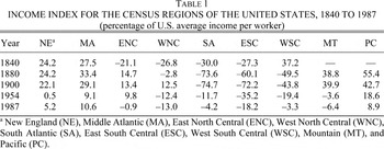
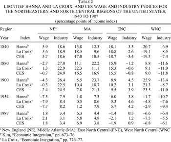
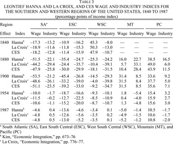
La Croix proved that Kim's analysis of U.S. regional development did not produce unique and conclusive results. To address this problem I developed the CES income index that provides unique and exact wage and industry indices. Table 1 gives an overview of the trends in regional income per worker compared to the U.S. average between 1840 and 1987. From these measures, the effects of wages paid and industry mix can be attributed. Tables 2 and 3 presents the Leontief Hanna and La Croix, and CES wage and industry indices for the nine census regions of the United States. This information is used to address the contradictions raised by La Croix about Kim's conclusions.
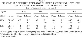
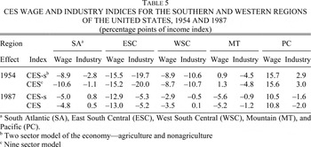
Beyond the issues raised by La Croix, I address several others in addition. Tables 4 and 5 show the effects that different number of sectors have on the size of the wage and industry indices in 1954 and 1987. Aggregating sectors together implies they are perfect complements. I hypothesize that the more industries aggregated together the higher the wage effect because high- and low-wage industries are represented in the data as if they are one industry when aggregated into the same sector. “The use of the broad industrial categories, agriculture and nonagricultural, or even the one-digit industries, may attribute greater importance to wages in explaining regional differences in income per capita than is deserved.”29
Kim, “Economic Integration,” p. 671.
On the other hand, a too disaggregated sectoring scheme may treat labor in sectors that are perfect complements as if they were imperfect substitutes. This situation would also result in an overstatement of the labor substitution effect of wages.
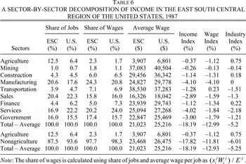
Table 6 displays the wage and income effects of each sector in the East South Central region in 1987 using schemes of both two and nine sectors.
I reviewed the conclusions in which Kim and La Croix were in agreement to see if they are still true in light of the CES income index approach. First Kim states that “the most significant cause of income divergence between 1840 and 1900 was the sharp relative decline in Southern income per capita caused by the region's growing unfavorable industry mix and lower wages relative to other regions.”30
Kim, “Economic Integration,” p. 672.
From
Table 1, we see that the Southern region of the South Atlantic, East South Central, and West South Central regions had the lowest per worker income of the nation from 1840 to 1900.
Table 3 shows that the South Atlantic region had a higher proportion of low wages, East South Central had about equal proportion of low wages and lower paying jobs, and the West South Central region had a larger portion of lower paying jobs. The CES wage and industry measure reconciles the slight disparities in the Hanna and La Croix indices in this region over this time period.
La Croix also agreed with Kim's conclusion that, “for all regions in 1954 the income differences that can be attributed to the industry-mix effects were considerably lower than they were in 1900.”31
Kim, “Economic Integration,” p. 677.
This conclusion means that the absolute value of the industry index in 1900 is greater than that for 1954 for all regions. From
Tables 2 and
3 we see that this statement is true relative to the Hanna index that Kim calculated. However in the East North Central region both the La Croix and CES industry indices show that the industry effect was greater in 1954 than in 1900. La Croix also notes this exception.
32 La Croix, “Economic Integration,” p.775.
Third Kim says, “the favorable industry-mix income effect for the New England and Middle Atlantic regions fell from 25 percent to less than 10 percent between 1900 and 1954.”33
Kim, “Economic Integration,” p. 677.
The results in
Table 2 show that between 1900 and 1954 the advantage in industry mix in New England and the Middle Atlantic regions fell from 25 and 21 percent to 8 percent respectively.
Next we turn to the conclusions by Kim that La Croix questioned. Kim states: “for some regions, such as the New England and Middle Atlantic regions, favorable regional industrial structures were responsible for their relatively high aggregate income per capita. For other regions, such as the Mountain and Pacific regions, their relatively high aggregate incomes were attributed to favorable wages.”34
Kim, “Economic Integration, pp. 671-72.
La Croix found that “The wages and industry-mix decompositions for the Middle Atlantic region in 1880 produced completely different results Kim's industry-mix decomposition shows that 66.6 percent of the income differential for the Middle Atlantic regions is due to favorable industry mix …”
35 La Croix, “Economic Integration, pp. 777-78.
From
Table 2 we see that in New England region, the wage index is less than the industry index in all five time periods. In the Middle Atlantic region, wage effects are less than industry effects in 1900 and 1954; wages are greater in 1840 and 19987; and they are the same in 1880. In the Mountain region the wage index is greater than the industry index in two the four time periods -1900 and 1954. In the Pacific regions, the wage effect is always greater than the industry effect. So Kim's conclusion holds for New England and Pacific but not for Middle Atlantic and Mountain regions.
Fifth, Kim states: “lower relative wages were more important than unfavorable industry-mix in explaining the relative decline in the income per capita of the South Atlantic and East South Central regions” in 1880 and 1900.36
Kim, “Economic Integration,” p. 672.
La Croix on the other hand found that “unfavorable industry mix explains a larger percentage of the East South Central region's income differential in 1880 and 1900 than lower relative wages.”
37 La Croix, “Economic Integration,” p. 778.
From
Table 3 we know that the wage effect was more negative than the industry effect in the South Atlantic region in both 1880 and 1900. In the East South Central region the wage and industry effects were equally negative in 1880. By 1900 the wage effect became more negative in the East South Central region. Kim's conclusion is true for the South Atlantic region only.
Kim concludes: “by 1987 differences in regional industrial structure accounted for only a small fraction of the differences in earnings.”38
Kim, “Economic Integration,” p. 677.
La Croix states that: “the average absolute value of the industrial mix differential falls from over 11 percent in both decompositions [in 1840] to 2.5 percent in Kim's decomposition and 2.7 percent in La Croix's decomposition [in 1987].”
39 La Croix, “Economic Integration,” p. 778.
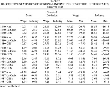
The range of the industry index for the seven regions in 1840 is from 19 to −16 percent and has a standard deviation of 13. By 1987 the range for the industry effect for the nine regions is 4 to −6 percent with a standard deviation of about 3. Kim's conclusion is correct. See
Table 7.
Does the number of sectors make a difference in the measure of the wage and industry effects? See Tables 4 and 5. In 1954 five of the nine regions had lower wage indices when the results were based on a nine-sector model of the economy. In 1987 four of the nine regions had lower wages indices with more sectors. The sectoring scheme had the biggest effect on the wage and industry indices in the East North Central, West North Central, and South Atlantic regions in 1954. In general, however, the aggregation scheme of the economy did not affect to the wage and industry indices beyond what might have happened by chance.
In 1987 the East South Central region had the lowest relative per worker income in the nation at minus eighteen percent. From Table 3 we know that 13 percentage points are wage effects. Which sectors were paying such low wages? See Table 6. Low wages in manufacturing, services, government, and sales (wholesale and retail) are responsible for about half of the low income per worker in the region. If we had only the two-sector model, all we could say is that low wages in the nonagriculture sector were responsible for about 12 percent points of the low income in the region.
CONCLUSIONS
This note has taken up the challenge of developing an approach that not only resolves the Hanna and La Croix index inconsistency problem but also explains why it happens. In the process I have developed an index that generates exact measures of each sector's contribution to the wage and industry effects of the region.
A wage index method was developed based on an assumed CES income function. An exact wage index as a second-order approximation of the income function was derived using a Taylor series expansion. From Hotelling's lemma, we know that the first derivative of a CES income function equals the wage share. With these insights, the original Hanna and La Croix income indices were reverse engineered to show that they are first-order approximations of an assumed Leontief income function. The Leontief Hanna and La Croix indices are also based on the assumption that the first derivative of the linear income function equals the labor share. With all these problems why are the Leontief Hanna and La Croix indices as accurate as they are? Diewert's lemma is used to demonstrate that the average of two first-order wage approximations of the income function equals the exact CES wage index. The average of the Leontief Hanna and La Croix indices is a first-order approximation of a CES income function. Because the Leontief indices are linear and the first-order CES approximations are tangents and also linear, the average of the original Hanna and La Croix wage indices is approximately equal to the exact CES wage index. However, only a second-order estimate of a CES function gives a unique and exact wage and industry measures of the function in total and for each sector.
Kim and La Croix agree on half of Kim's six conclusions about the convergence in earnings across regions of the United States. For the three conclusion upon which they agreed we found some additional information and support. A disparity to Kim's conclusion that “the most significant cause of income divergence between 1840 and 1900 was the sharp relative decline in Southern income per capita caused by the region's growing unfavorable industry mix and lower wages relative to other regions” was reconciled. La Croix's insight that the East North Central region is an exception to the conclusion that “for all regions in 1954 the income differences that can be attributed to the industry-mix effects were considerably lower than they were in 1900” was verified. Finally, the conclusion that “the favorable industrial-mix income effect for the New England and Middle Atlantic regions fell from 25 to less than 10 percent between 1900 and 1954” was sharpened. The actual amounts were 25 and 21 percent to 8 percent.
For the conclusions on which Kim and La Croix disagreed the following emerged: Only New England on the one hand and the Pacific regions on the other support Kim's conclusion that “some regions” have consistently favorable industrial structure while others have consistently favorable wages to explain higher income per worker. Next only the South Atlantic region has results that supports Kim's conclusion that lower wages were more important than unfavorable industry-mix in explaining the relative decline in per capita income in both the South Atlantic and East South Central regions in 1880 and 1900. Finally, Kim's conclusion that the industry effect was significantly less in 1987 than in 1840 was confirmed. The results show that it took about a century to overcome the effects of the Civil War and for industrialization to change comparative advantage enough so that regional incomes converged beyond those of the U.S. agricultural economy of the 1840s. Krugman states that “increasing returns are … a pervasive influence on the economy, and that these increasing returns give a decisive role to history in determining the geography of real economies.”40
Krugman, “Geography,” p. 10.
His theory is both supported and refuted by these results. It is right that location is destiny in the sense of maintaining rank order. However the variance in this difference between regions decreases over time.
Finally we found that number of sectors used to calculate the wage and industry effects did not affect these measures beyond that of chance for the years 1954 and 1987. Though it is true in this instance, we would caution that this may not be true in all cases. Also the CES index can provide insight into the source of wage and industry effects by sector. In the case of East South Central region in 1987, for example, half of its 18 percent lower income compared to the U.S. can be attributed to particularly low wages in the manufacturing, service, government, and sales sectors.
Perhaps the overarching contribution of the CES wage index is that it allows interesting economic development stories to be told now without the shadow of index theory error cast over the conclusions. Also, by knowing the contribution of individual sectors, the CES wage and industry indices can provide exact and detailed insights into the history of economic development.