2.1. Computational domain and boundary conditions

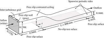
The computational domain used in the present study, shown in figure 1, consists of a contoured ceiling above a flat, no-slip test surface of length $L=800~\text{mm}$ . The streamwise contour of the ceiling produces a converging and diverging flow path over the test surface, thus imposing a streamwise pressure distribution on the test surface that resembles the pressure distribution on the suction side of an airfoil, specifically that of a low-pressure axial turbine blade. The use of a free-slip condition at the contoured ceiling allows a coarser wall-normal grid resolution near the ceiling and also ensures the absence of flow separation in the adverse pressure gradient region. The height of the ceiling above the test surface is 0.230 $L$ at the inlet, 0.168 $L$ at the outlet and 0.114 $L$ at the suction-peak location, which results in the ceiling height being always more than 50 times the local value of the boundary layer displacement thickness, ${\it\delta}^{\ast }$ , above the test surface. The inflow boundary consists of a $9\times 8$ array of square shaped jets of 9.3 mm width spaced 13.1 mm apart (centre to centre), which approximates the configuration of a turbulence generating grid. A uniform streamwise velocity of $11.5~\text{m}~\text{s}^{-1}$ is defined at each square shaped jet. Free-slip walls are specified between the square shaped jets owing to the difficulty in resolving the wall shear layers on the bars of the turbulence grid. A free-slip region of 0.566 $L$ length is located between the inflow boundary and the leading edge of the test surface to ensure that the free stream turbulence recovers from the limited resolution of the shear layers surrounding the square shaped jets and to allow the grid generated free stream turbulence to decay to the desired intensity and length scale. As detailed in § 3.1, this length also ensures that the free stream turbulence entering the test surface region is adequately isotropic and homogeneous. A free-slip surface of $0.165L$ length is located downstream of the test surface to place the outflow boundary a conservative distance from the region of interest, as the boundary condition at the outflow boundary condition distorts convective flow structures such as turbulent eddies as they exit the domain. Static pressure that remains fixed in an area-averaged sense at 0 Pa (gauge) is specified at the outflow boundary. Spanwise periodicity is imposed along the sides of the computational domain and a spanwise width of $S=0.125L$ is chosen to place the sides of the domain a conservative distance away from the region of interest, which is located near the midspan. To verify insensitivity of the results to the spanwise width of the domain, the simulation was repeated with a spanwise width of 0.25 $L$ . No observable differences were observed in boundary layer properties and transition development.

Figure 1.

Schematic of the computational domain (not to scale).

2.2. Spatial grid

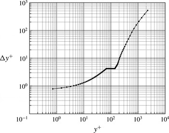
A structured grid consisting of hexahedral finite volumes is mapped to the computational domain shown in figure 1. To accurately perform a DNS of the flow in the current study, the spatial and temporal grids must be sufficiently refined to capture the smallest scales of the flow, which are on the order of the Kolmogorov length and time scales. For turbulent boundary layers, the Kolmogorov length scale is on the order of the viscous length scale, reaching a minimum value of ${\it\eta}^{+}\approx 2$ close to the no-slip boundary (e.g. Kim, Kline & Reynolds Reference Kim, Kline and Reynolds1971; Pope Reference Pope2000; Stanislas, Perret & Foucaut Reference Stanislas, Perret and Foucaut2008). In the following, normalization by wall units is indicated with a $+$ superscript, calculated using the maximum local wall shear stress observed in the time-averaged simulation results, which occurs at $x/L=0.785$ . The nodes are distributed such that the node spacing yields values of ${\rm\Delta}x^{+}=11$ and ${\rm\Delta}z^{+}=8$ , corresponding to approximately 4–5 times the Kolmogorov length scale at the target Reynolds number. The $y^{+}$ value of the nodes adjacent to the no-slip wall is less than 0.8 everywhere. In the range $0.8<y^{+}<30$ , the wall-normal node spacing is increased linearly from the value adjacent to the wall to a value that corresponds to the Kolmogorov length scale in the log-law region, which is approximated by:

where ${\it\kappa}=0.41$ is the von-Kármán constant (Pope Reference Pope2000; Stanislas et al. Reference Stanislas, Perret and Foucaut2008). Beyond $y^{+}=30$ , the node spacing is increased at a rate of 4 % until $y^{+}=70$ . The grid spacing remains constant in the range $70<y^{+}<140$ , and is then increased at a rate of 10 % until the free-slip ceiling of the domain is reached. This wall-normal node distribution is shown in figure 2.

Figure 2.

Wall-normal node distribution.

To resolve the free stream turbulence generated upstream of the test surface, a uniform streamwise node spacing of ${\rm\Delta}x^{+}=11$ is imposed between the inflow plane and the test surface leading edge. Uniform wall-normal and spanwise node distributions are imposed at the inflow plane such that 32 nodes occur in the $y$ and $z$ directions within each square shaped jet. The rectangular free-slip regions between the square shaped jets are resolved with 13 nodes along the short axis and 32 nodes along the long axis. Between the inflow plane and the test surface leading edge, linear interpolation with respect to the streamwise coordinate is used to modify the wall-normal node distribution in the downstream direction so that the distribution at the leading edge of the test surface matches that shown in figure 2. To ensure that the spatial grid does not affect the characteristics of the simulated free stream turbulence, the simulations were repeated with twice the number of nodes in the $y$ and $z$ directions. Negligible differences were observed between the refined grid results and the initial resolution results that are presented in § 3.1.

2.3. Solution method

Discretization of the incompressible mass and momentum conservation equations is based on central differencing and second-order Euler backward differencing for the spatial and temporal derivatives, respectively. A time step size of ${\rm\Delta}t=3.5\times 10^{-5}~\text{s}$ or 0.19 $t^{+}$ is used, where $t^{+}={\it\nu}/u_{{\it\tau}}^{2}$ is the viscous time scale at the time-averaged location of maximum wall shear stress, which is close to the time step size of 0.20 $t^{+}$ recommended by Choi & Moin (Reference Choi and Moin1994) for accurately computing turbulent flows. As an a posteriori check that the selected time step is suitable for resolving the time scales of the grid generated free stream turbulence, the time step size is compared to the computed Kolmogorov time scale of the free stream turbulence occurring just upstream of the test surface leading edge:

where ${\it\epsilon}$ is the local turbulent dissipation rate computed from the simulation. The selected time step size is approximately 0.008 ${\it\tau}_{{\it\eta}}$ , which suggests that the time scales of the free stream turbulence are properly resolved in the simulation.

Starting from a uniform static pressure of 0 Pa gauge and streamwise velocity of $4~\text{m}~\text{s}^{-1}$ , solution convergence of the discretized equations at each time step is obtained, with outer iteration loops serving to converge the coefficients of the linearized governing equations and inner iteration loops facilitating the solution of these equations through W-type algebraic multigrid cycles. Six grid levels are used in the multigrid cycle with one solution sweep performed at each grid level during the restriction passes and three solution sweeps performed at each grid level during the prolongation passes. The transient solution is obtained with one inner loop iteration per outer loop iteration, and multiple outer loop iterations per time step. For each time step, the solution is declared as converged when the root-mean-square residuals of the governing equations are reduced by five orders of magnitude to less than $10^{-6}$ . 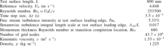This is realized with up to eight outer loop iterations per time step. Approximately 10 flow through times are required for the flow to reach a statistically steady state, after which approximately 13 000 time steps (approximately three flow through times) are computed for analysis. The simulation was partitioned and executed in parallel on 24 cores of AMD Opteron 6128 processors. Details of the simulation are given in table 1.

Table 1.

Flow conditions and numerical details of the current simulation.

2.4. Validation of numerical approach

Validation of the numerical algorithm and the spatial and temporal resolutions is accomplished by performing a series of companion DNS studies of a temporally developing zero pressure gradient turbulent boundary layer and comparing the results of these simulations to statistical turbulence properties of corresponding turbulent boundary layers available in literature. The dimensions of the computational domain for the companion simulations are 670, 1820 and 650 viscous units in the $x$ , $y$ and $z$ directions, respectively, and is spatially periodic in the streamwise ( $x$ ) and spanwise ( $z$ ) directions. The companion simulations are initialized with a spatially uniform velocity of $1.6~\text{m}~\text{s}^{-1}$ and the boundary layer is developed in time until a momentum thickness Reynolds number of $Re_{{\it\theta}}=700$ is reached. Transition is triggered at $Re_{{\it\theta}}=450$ through a mass source/sink pair lasting 4.5 $t^{+}$ that is located near the wall in the centre of the domain that injects fluid into the domain at a wall-normal velocity of $0.16~\text{m}~\text{s}^{-1}$ . 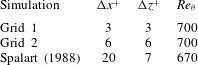The spatial resolutions of the complementary DNS studies are listed in table 2. The Reynolds number was chosen to match the momentum thickness Reynolds number at the transition completion location of the present bypass transition simulation, as listed in table 1. Considering that the transient flow structures in a fully turbulent boundary layer have a larger range of spatial and temporal scales than a transitional boundary layer at a comparable Reynolds number, the companion studies provide a rigorous case for validating the numerical approach of the present bypass transition simulations.

Table 2.

Computational grids for the validation studies.

Figure 3.

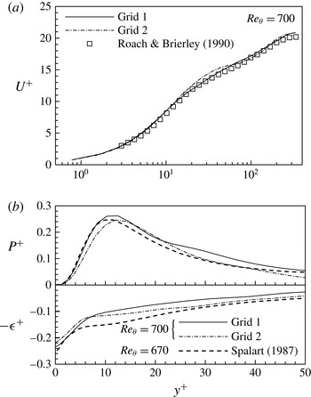
Validation DNS study of a zero pressure gradient turbulent boundary layer at $Re_{{\it\theta}}=700$ . (a) Mean velocity profile. (b) Turbulence production and dissipation rate budgets.

The first validation simulation (Grid 1) was performed with a spatial resolution in the $x$ – $z$ plane of ${\rm\Delta}x^{+}={\rm\Delta}z^{+}=3$ , which corresponds to about 1.5 times the Kolmogorov length scale at this Reynolds number. The $y^{+}$ value of the first node from the no-slip boundary is 0.85 and the wall-normal node distribution follows closely the distribution shown in figure 2. Figure 3 shows that the results achieve very good agreement with the turbulent mean velocity profile measured experimentally by Roach & Brierley (Reference Roach, Brierley, Pironneau, Rode and Ryhming1990) and the turbulence kinetic energy production and dissipation rate budgets (denoted $P^{+}$ and ${\it\epsilon}^{+}$ , respectively) computed by Spalart (Reference Spalart1988), who used an algorithm utilizing a spectral method for spatial discretization and a second-order accurate hybrid Runge–Kutta/Crank–Nicholson scheme for temporal discretization to simulate the boundary layer at a Reynolds number of $Re_{{\it\theta}}=670$ . The slight disagreement that is observed in the dissipation rate budget is comparable to variation that exists in published literature at $Re_{{\it\theta}}=700$ due to differences in the way each study triggers transition to turbulence. To ascertain the sensitivity of the results to the spatial resolution, a second validation DNS (Grid 2) with a grid that closely matches the spatial resolution of the present study was performed at $Re_{{\it\theta}}=700$ . In comparison to the Grid 1 results shown in figure 3, the coarser grid achieves a similar level of agreement with published results. Therefore, these validation studies provide strong evidence that the present study should accurately capture the flow development in a bypass transition scenario. As per figure 3, although the Grid–1 results are in slightly better agreement with the simulation data of Spalart (Reference Spalart1988) and the experimental data of Roach & Brierley (Reference Roach, Brierley, Pironneau, Rode and Ryhming1990) than the Grid–2 results, the resolution of Grid–2 was adopted for the present simulations to achieve reasonable computing times while still ensuring that the flow physics are accurately captured.

3.1. Free stream flow development

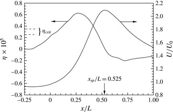
As described in § 2.1, the free stream flow is generated through a periodic array of square shaped inflow boundaries in a $y$ – $z$ plane located 0.566 $L$ upstream of the test surface leading edge, which resembles the turbulence generating grids studied by Roach (Reference Roach1986). The streamwise distribution of the mean streamwise velocity of the free stream flow is shown in figure 4 by plotting the streamwise velocity averaged in time, denoted as $U$ . The flow development upstream of $x/L=-0.25$ is not shown because the flow has not mixed out to a sufficient extent following the turbulence generating inflow condition to yield a satisfactorily steady flow. The streamwise acceleration parameter, ${\it\eta}={\it\nu}/U^{2}(\text{d}U/\text{d}x)$ , is also shown to illustrate the degree of streamwise acceleration present in the free stream flow. The two dashed horizontal lines in figure 4 identify the critical range of the acceleration parameter, beyond which several researchers have observed that a turbulent boundary layer will begin to relaminarize (Moretti & Kays Reference Moretti and Kays1965; Jones & Launder Reference Jones and Launder1972; Escudier et al. Reference Escudier, Abdel-Hameed, Johnson and Sutcliffe1998). Figure 4 shows that the majority of the flow between the test surface leading edge and the suction peak location ( $x_{sp}/L=0.525$ ) is accelerated at a level well above the critical value for relaminarization, which implies that any disturbances penetrating into the boundary layer or developing in the boundary layer via viscous instability modes are expected to be damped in this region.

Figure 4.

Streamwise distributions of free stream velocity, $U/U_{0}$ , and acceleration parameter,  ${\it\eta}$ . The suction peak location is denoted $x_{sp}$ .

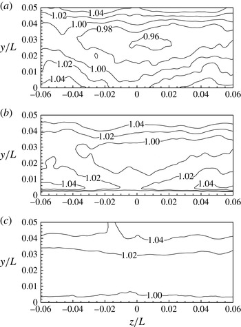
The degree of spatial uniformity of the free stream velocity is shown in figure 5 by plotting contours of the temporally-averaged local streamwise velocity, $U$ , in several $y$ – $z$ planes, where $U$ is normalized by the free stream velocity averaged over the local $y$ – $z$ plane, which is denoted $U_{yz}$ . Just upstream of the test surface leading edge, at $x/L=-0.004$ , the non-uniformity is about 0.08 $U_{yz}$ , and this non-uniformity is attributed to the incomplete mixing of the free stream flow downstream of the turbulence generating grid. The incomplete mixing is partially due to the spanwise periodic boundary conditions that are applied on the side walls of the subdomains upstream of the test surface leading edge. As the computational algorithm does not preserve continuity in the first derivatives of flow variables across a periodic boundary, eddies passing through the periodic boundaries are deformed and thus the turbulence grid wakes located near the periodic side walls have a slightly altered mixing rate compared to those located near the centre of the domain. As will be shown, this numerical artefact does not significantly influence the statistical properties of the free stream turbulence and their agreement with published literature. Downstream of the test surface leading edge, at $x/L=0.121$ , the free stream non-uniformity begins to decrease as the free stream is accelerated by the pressure distribution imposed by the contoured ceiling. By $x/L=0.371$ , the non-uniformity is less than 0.04 $U_{e}$ and occurs far away from the boundary layer edge such that the flow near the wall shear layer (below $y/L=0.02$ ) is spatially uniform to within 0.004 $U_{e}$ . The free stream non-uniformity observed in figure 5 is taken into account in the remaining discussion by defining the mean flow field as the spanwise average of the temporally-averaged flow field, and the spanwise averaging is performed only on the free stream flow below $y/L=0.02$ and between $z/L=-0.03$ and 0.03.

Figure 5.

Contours of $U/U_{yz}$ in $y$ – $z$ planes at (a) $x/L=-0.004$ , (b) $x/L=0.121$ and (c)  $x/L=0.371$ .

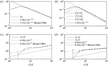
The decay of the free stream turbulence downstream of the simulated turbulence grid is shown in figure 6. In this figure, $x^{\prime }$ is the streamwise coordinate referenced to the inflow plane. The quantities in figure 6 are spatially-averaged in the aforementioned manner at each streamwise location, and the uncertainty in the spatial mean values is shown by the error bars. For improved clarity, the error bars are plotted at only selected $x^{\prime }/d$ locations. The error bars qualitatively indicate that the degree of spatial non-homogeneity of the free stream turbulence is small near the leading edge of the test surface; when estimated as the standard error of the value of $Tu$ in a plane located at $x/L=-0.004$ ( $x^{\prime }/d=117.8$ ), the spatial non-homogeneity is less than 1 % of the spatially-averaged value of turbulence intensity in that plane.

Figure 6.

Streamwise decay of free stream turbulence upstream of the test surface. Area-averaged distribution of (a) turbulence intensity, $Tu$ , (b) normal Reynolds stresses and (c,d) integral length scales. Error bars indicate uncertainty in the spatial mean values.

The validity of the present method for generating free stream turbulence is further assessed by comparing the properties shown in figure 6 with semiempirical correlations developed by Roach (Reference Roach1986) for grid-generated free stream turbulence. The grid Reynolds number is $Re_{d}=1211$ , which is within the range considered by Roach (Reference Roach1986). The turbulence intensity is plotted in figure 6(a), defined as $Tu=\sqrt{1/3(\overline{u^{\prime 2}}+\overline{v^{\prime 2}}+\overline{w^{\prime 2}})}/U_{0}$ , where the prime indicates fluctuation values. The Reynolds normal stresses and turbulence integral length scales are shown in figure 6(b–d). Trend lines in figure 6 are determined through a least-squares fit to the data that lies in the range $x^{\prime }/d=30{-}118$ , where the turbulence is most fully developed. The correlations proposed by Roach (Reference Roach1986) are also plotted to facilitate comparison with the present results. Figure 6(a) shows that after an initial growth period immediately downstream of the simulated grid, $Tu$ decays exponentially in agreement with the correlation proposed by Roach (Reference Roach1986). The turbulence integral length scales in figure 6(c,d) are calculated by integrating the normalized autocovariance function of the fluctuating streamwise velocity component in the three coordinate directions:

where $r$ is oriented in the $x_{i}$ direction. By about 30 $d$ downstream of the inflow plane, the streamwise integral length scale of the free stream turbulence (figure 6 c) grows according to $0.50(x/d)^{1/2}$ . This agrees favourably with the correlation of Roach (Reference Roach1986) in terms of the streamwise growth rate but is offset vertically. The offset is attributed to differences in the initial state of the generated turbulence; the boundary layers around the bars of the turbulence generating grid are not resolved in the present study, which results in the openings of the numerical turbulence grid being slightly larger than in an experimental turbulence grid of the same geometry. While this does not alter the mechanisms of the free stream turbulence decay, demonstrated particularly by the agreement of the streamwise growth rates in the length scales, it does alter the initial length scales of the generated free stream turbulence and results in the noted differences in the correlation constants. The large uncertainty in the integral length scales at low $x/d$ values is due to wakes behind the closed portions of the simulated turbulence grid, which create large spatial non-uniformities in the turbulence scales that diminish as the wakes dissipate. The integral length scales in the $y$ and $z$ coordinate directions (figure 6 d) grow at a lower rate than the streamwise length scales. This is likely due to the manner by which the free stream turbulence is generated in the present study, which as per figure 4 influences the free stream flow up to about $x/L=-0.25$ or $x^{\prime }/d=60$ . The Reynolds normal stresses plotted in figure 6(b) illustrate a slight anisotropy in the free stream turbulence. The streamwise fluctuation levels are approximately 10 % and 20 % higher than fluctuations in the $y$ and $z$ coordinate directions, respectively, which is consistent with the observations of Roach (Reference Roach1986) in similar configurations.

Figure 7.

Frequency spectrum of the fluctuations in the streamwise component of velocity at $x/L=-0.035$ .

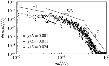
Figure 7 plots the frequency spectrum of the fluctuations in the streamwise component of velocity in the free stream at $x/L=-0.035$ , just upstream of the leading edge of the test surface. The turbulence at this location is representative of the free stream turbulence to which the test surface boundary layer is exposed. The power spectral density, ${\it\phi}({\it\omega})$ , and frequency, ${\it\omega}$ , in figure 7 are normalized by the turbulence bar width, $d$ , and reference velocity, $U_{0}$ . The power spectra at three wall-normal locations are plotted to illustrate the variation in the turbulence spectrum at a range of wall-normal heights, which figure 7 shows to be minimal. Three distinct ranges are observed in the power spectra: a ${\it\omega}^{-1}$ range at low frequencies followed by a ${\it\omega}^{-5/3}$ range at intermediate frequencies, which matches the experiments of Klebanoff (Reference Klebanoff1954), and a ${\it\omega}^{-7}$ range at high frequencies that is also observed in a recent DNS by Hickey et al. (Reference Hickey, Blakie, Gray and Wu2010).

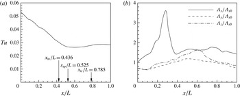
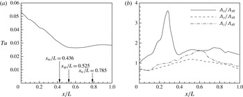
The development of free stream turbulence downstream of the test surface leading edge is illustrated in figure 8. The decrease in the turbulence intensity and the increase in the ${\it\Lambda}_{x}$ length scale upstream of the suction peak location is promoted by the strong free stream acceleration, which dampens the free stream eddies while stretching them in the $x$ direction. The maximum in the ${\it\Lambda}_{x}$ distribution at approximately $x/L=0.3$ coincides with the location of maximum free stream acceleration as per figure 4. Downstream of this location, the streamwise-elongated eddies experience a lesser degree of streamwise acceleration on their downstream sides than on their upstream sides so that the eddy is ‘squeezed’ and ${\it\Lambda}_{x}$ decreases. Downstream of the suction peak, the streamwise variation in the turbulence intensity and length scales is greatly reduced. As a result, the majority of the transitional region of the test surface occurs under relatively uniform free stream turbulence conditions with an intensity of 0.026–0.028 $U_{0}$ and integral length scales of 0.013 $L$ –0.027 $L$ .

Figure 8.

Streamwise decay of free stream turbulence downstream of the test surface leading edge. Area-averaged distribution of (a) turbulence intensity, $Tu$ , (b) integral length scales normalized by ${\it\Lambda}_{x0}$ , the streamwise integral length scale at the test surface leading edge.

3.2. Test surface boundary layer development

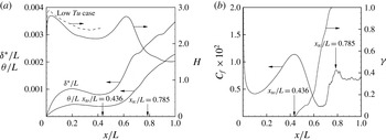
The development of the test surface boundary layer is plotted in figure 9(a) through streamwise distributions of the boundary layer integral parameters. The time-averaged locations of transition onset ( $x_{to}/L=0.436$ ) and completion ( $x_{tc}/L=0.785$ ) are also shown. From figure 9(b), the transition onset location is determined through the intermittency parameter, ${\it\gamma}$ , defined as the percentage of time the boundary layer is turbulent. The intermittency parameter distribution is computed using the algorithm of Volino, Schultz & Pratt (Reference Volino, Schultz and Pratt2001). The transition completion location is determined by the local maximum in the friction factor, $C_{f}=2{\it\tau}_{w}/{\it\rho}U_{0}^{2}$ , which also agrees well with the streamwise location where ${\it\gamma}=1$ .

The effect of the free stream turbulence on the boundary layer integral parameters is deduced by comparing the shape factor ( $H$ ) distribution in figure 9(a) to the $H$ distribution that would occur under low free stream turbulence levels. To obtain such a low turbulence $H$ distribution, a complementary simulation was performed in which the turbulence generating grid of the present study is replaced with a uniform inlet velocity equal to $U_{0}$ . The streamwise velocity distribution in the free stream of the low turbulence simulation is identical to the present high turbulence case in the region upstream of the transition onset location. However, figure 9(a) shows that the $H$ distribution that occurs under low free stream turbulence is consistently larger than in the present high turbulence case, which is consistent with previous experimental data of the authors’ research group (e.g. Roberts & Yaras Reference Roberts and Yaras2005). The difference in the $H$ distribution under low and high free stream turbulence levels suggests that free stream turbulence introduces small, localized perturbations into the laminar boundary layer that yield Reynolds stresses within the boundary layer; this is described in more detail in § 3.3. The mixing associated with the Reynolds stresses fills out the velocity profile of the boundary layer under high free stream turbulence relative to the boundary layer under low free stream turbulence, producing lower values of  $H$ . Downstream of the suction peak ( $x_{sp}/L=0.525$ ), the transition rate increases – indicated by the ‘kink’ near this location in the ${\it\gamma}$ distribution – and $H$ eventually reaches a steady value of about 1.5 in the fully turbulent boundary layer.

Figure 9.

Streamwise distributions of (a) displacement thickness ( ${\it\delta}^{\ast }/L$ ), momentum thickness ( ${\it\theta}/L$ ) and shape factor ( $H$ ); (b) friction factor ( $C_{f}\times 10^{2}$ ) and intermittency ( ${\it\gamma}$ ). The $H$ distribution for a complementary low free stream turbulence simulation is shown in (a) with dashed lines.

3.3. Formation and properties of boundary layer streaks

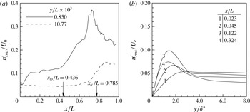
Longitudinal low-speed streaks are created in the laminar boundary layer through the selective inclusion of disturbances from the free stream beginning near the test surface leading edge (Jacobs & Durbin Reference Jacobs and Durbin2001). This is seen in figure 10(a) by plotting the streamwise distributions of root-mean-square streamwise fluctuation velocity, $u_{rms}^{\prime }/U_{0}$ , at wall-normal locations of $y/L=10.77\times 10^{-3}$ and $0.850\times 10^{-3}$ . Within the laminar flow region between $x/L\approx 0.1$ and 0.5, these locations roughly correspond to $y\approx 10{\it\delta}^{\ast }$ and $y\approx 1{\it\delta}^{\ast }$ , respectively, and so are respectively representative of the conditions in the free stream and well within the boundary layer. The distribution in the free stream initially shows a slight decreasing trend in $u_{rms}^{\prime }$ due to the enhanced decay of free stream turbulence and flow stabilization by the imposed favourable pressure gradient. Past the transition completion location, the free stream flow experiences an increase in $u_{rms}^{\prime }$ due to the influence of disturbances from the turbulent boundary layer. In contrast, the boundary layer $u_{rms}^{\prime }$ distribution experiences an abrupt increase in fluctuation strength near $x/L=0.03$ as free stream disturbances penetrate the boundary layer and are amplified via a transient growth mechanism. The fluctuations reach a steady amplitude by around $x/L=0.1$ and do not grow significantly until the transition onset location is reached. Although not shown, the root-mean-square of the wall-normal velocity fluctuations within the boundary layer is the same order of magnitude as the streamwise fluctuations. The associated Reynolds stresses produce the lower values of $H$ in the laminar boundary layer relative to the low free stream turbulence case that was noted in § 3.2. The fluctuation amplitude increases rapidly within the transition zone due to the nonlinear processes described in § 3.4, reaching a peak amplitude near the transition completion location, and then decreases as the flow becomes fully turbulent.

Figure 10.

(a) Streamwise distribution of $u_{rms}^{\prime }$ at $y/L=0.850\times 10^{-3}$ and $y/L=10.77\times 10^{-3}$ . (b) Wall-normal profiles of $u_{rms}^{\prime }$ in the laminar region.

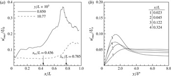
The initial fluctuation growth in the laminar boundary layer is examined in figure 10(b) through wall-normal profiles of $u_{rms}^{\prime }$ normalized by the local boundary layer edge velocity, $U_{e}$ . The wall-normal coordinate is normalized by the local displacement thickness, ${\it\delta}^{\ast }$ , which is between 40 % and 80 % of the local boundary layer thickness. Profile 1 shows that near the leading edge ( $x/L=0.023$ ), the fluctuation strength monotonically decreases from the turbulent free stream towards the wall with negligible amplification of disturbances in the boundary layer. Profile 2 shows that by $x/L=0.045$ , free stream disturbances have penetrated the boundary layer and have begun to be amplified, seen through the increase in peak $u_{rms}^{\prime }$ at $y/{\it\delta}^{\ast }=2$ . The location of the disturbance growth relative to the boundary layer edge indicates that the disturbances are not amplified through a viscous Tollmien–Schlichting (T–S) instability mode, in which the maximum amplification is located near to the wall (e.g. Reynolds & Saric Reference Reynolds and Saric1986), but through a transient growth mechanism of the free stream disturbances. Downstream of profile 3, the acceleration imposed by the favourable pressure gradient causes the fluctuation amplitude to decrease slightly relative to the local edge velocity, seen by profile 4 at $x/L=0.324$ , although figure 10(a) shows that the disturbance amplitude in an absolute sense remains relatively constant.

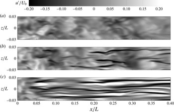
Figure 11 illustrates the form of the disturbances that penetrate into the boundary layer near the test surface leading edge. Contours of streamwise velocity fluctuations are plotted in the same wall-normal planes as in figure 10(a) plus an intermediate location at $y/L=2.950\times 10^{-3}$ which corresponds to about three times the local value of ${\it\delta}^{\ast }$ and is situated above the edge of the boundary layer within the plotted streamwise region. Figure 11(a) shows that the free stream turbulence consists of small-scale disturbances that are roughly isotropic in the visualized plane. As these disturbances penetrate into the boundary layer, they form streamwise elongated streaks that primarily consist of narrow $u<0$ fluctuations compensated by broader regions of $u>0$ fluctuations. The shear sheltering phenomenon observed by Jacobs & Durbin (Reference Jacobs and Durbin2001) is clearly distinguished by comparing the three wall-normal planes; the high-frequency free stream modes are visible near the leading edge in all three planes, but these are quickly damped within the boundary layer such that only the low-frequency streamwise streaks are amplified.

Figure 11.

Contours of the fluctuations in the streamwise component of velocity at (a) $y\approx 10{\it\delta}^{\ast }$ , (b) $y\approx 3{\it\delta}^{\ast }$ and (c)  $y\approx 1{\it\delta}^{\ast }$ : (a) $y/L=0.850\times 10^{-3}$ ; (b) $y/L=2.950\times 10^{-3}$ ; (c) $y/L=10.77\times 10^{-3}$ .

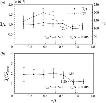
The statistical properties of the low-speed streamwise streaks are highlighted by analysing their spanwise spacing and amplitude. These properties have been shown to be closely connected to the development of secondary streak instabilities, as reviewed in § 1. Figure 12(a) plots the mean spanwise spacing of the low-speed streaks at several streamwise locations. The mean spanwise spacing, denoted $\overline{{\it\lambda}}$ , is calculated by averaging the centre to centre distance between streaks in a $y$ – $z$ plane at a particular streamwise location at four uniformly spaced instances in time, resulting in 50–150 streaks being included in the average at each streamwise station. The temporal spacing was large enough to ensure that unique streaks are used in the average at each instance in time. The error bars in figure 12(a) indicates the uncertainty in $\overline{{\it\lambda}}$ based on the standard error of the mean spacing. A larger uncertainty occurs near the leading edge due to an increased variance in ${\it\lambda}$ near the leading edge, primarily due to the free stream turbulence that triggers the streaks. Because the free stream turbulence is composed of disturbances with a broad spectrum of wavelengths, it is expected that the streaks will initially have a broad range of spacings. Once the free stream disturbances permeate into the boundary layer, the local conditions within the boundary layer determine what wavelengths will be amplified, and disturbances with non-optimum wavelengths are damped out. The variance in ${\it\lambda}$ thus decreases with downstream distance, as shown by the diminishing uncertainty bounds.

Figure 12.

Streamwise distribution of the spanwise spacing of the low-speed $u$ -velocity streaks. Normalization is by (a) $L$ and $u_{{\it\tau}}/{\it\nu}$ and (b) $\overline{{\rm\Delta}z}_{streak}$ .

Figure 12(a) shows that the absolute spanwise spacing of the low-speed streaks ( $\overline{{\it\lambda}}/L$ ) achieves an approximately constant value upstream of the transition completion location, followed by a lower value in the turbulent region. When normalized by the viscous length based on the local wall shear stress, the streak spacing increases until $x/L=0.371$ , which corresponds to the station with the strongest free stream acceleration and largest wall shear stress (figures 4 and 9). $\overline{{\it\lambda}^{+}}=198\pm 26$ is much larger than the typical spacing of $100\pm 20$ viscous lengths in zero pressure gradient turbulent boundary layers (Smith & Metzler Reference Smith and Metzler1983; Rajaee, Karlsson & Sirovich Reference Rajaee, Karlsson and Sirovich1995), implying enhanced stability of the boundary layer in the accelerated region (e.g. Yaras Reference Yaras2007). Downstream of $x/L=0.371$ , the normalized streak spacing decreases quite rapidly as the boundary layer reacts to the reduction in free stream acceleration, settling to values in the fully turbulent region that are in closer agreement to those in zero pressure gradient turbulent boundary layers. The increase in $\overline{{\it\lambda}^{+}}$ downstream of $x/L=0.620$ reflects the decrease in the wall shear stress in the turbulent region (as shown in figure 9), as $\overline{{\it\lambda}}/L$ changes very little.

Figure 13.

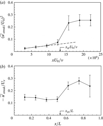
Streamwise development of the amplitude of the low-speed $u$ -velocity streaks. (a) Disturbance energy $(\overline{u^{\prime }}_{streak}/U_{0})^{2}$ ; dashed line, $(\overline{u^{\prime }}_{streak}/U_{0})^{2}=3.50\times 10^{-7}(xU_{0}/{\it\nu})$ . (b) Relative streak amplitude $\overline{u^{\prime }}_{streak}/U_{e}$ .

In figure 12(b), $\overline{{\it\lambda}}$ is normalized by the local width of the low-speed streaks, denoted $\overline{{\rm\Delta}z}_{streak}$ . The ratio $\overline{{\it\lambda}}/\overline{{\rm\Delta}z}_{streak}$ has been shown to be relevant in determining whether secondary instabilities of the streamwise streaks will develop (Konishi & Asai Reference Konishi and Asai2004). Mean streak widths are determined by individually examining each streak at the same streamwise locations and instances in time as those used in evaluating the streak spacing. For a given streak under examination, its width is determined based on the spanwise locations of the left and right spanwise edges of the streak, which are determined based on threshold values of $u^{\prime }/U_{e}$ . Three preliminary widths are calculated using threshold values of $u^{\prime }/U_{e}=0.03$ , 0.05 and 0.07, and these preliminary widths are averaged to give an individual mean streak width. The average of all such individual streak widths over the four even spaced instances in time corresponds to the local mean streak width, $\overline{{\rm\Delta}z}_{streak}$ . To ascertain the sensitivity of $\overline{{\rm\Delta}z}_{streak}$ to the threshold values of $u^{\prime }/U_{e}$ and the number of preliminary streak widths included in the averaging process, the above described method was repeated at selected axial locations using 2, 4 and 6 uniformly spaced threshold values between $u^{\prime }/U_{e}=0.02$ and 0.08. The resulting uncertainty in the width of an individual streak due to the choice of threshold values was found to be much smaller than the uncertainty in $\overline{{\rm\Delta}z}_{streak}$ due to the varied widths of all the streaks examined at a given axial location. This latter uncertainty is shown by the error bars in figure 12(b).

The trends visible in figure 12(b) indicate that $\overline{{\it\lambda}}/\overline{{\rm\Delta}z}_{streak}$ achieves distinct but approximately constant values of 1.94 and 1.20 in the laminar and turbulent regions, respectively, despite the range of boundary layer thicknesses and streamwise pressure gradients present in both regions. The low-speed streamwise streaks are, on average, spaced less than 2.5 streak widths apart, which Konishi & Asai (Reference Konishi and Asai2004) observed is the threshold spacing beyond which secondary instability modes are suppressed. This implies that, at least in terms of the streak spacing, the conditions along the whole test surface are suitable for the development of secondary streak instabilities. Time histories of the convecting streaks, however, show that neither symmetric (varicose) nor asymmetric (sinuous) secondary instabilities develop upstream of the suction peak. Figure 13 plots the amplitude and disturbance energy of the streaks at the streamwise stations corresponding to figure 12. The mean streak amplitude, $\overline{u^{\prime }}_{streak}$ , is defined as the local maximum of $|u^{\prime }|$ occurring in a low-speed streak, averaged over multiple streaks using the same method as was used for $\overline{{\it\lambda}}$ . The disturbance energy of the streaks $(\overline{u^{\prime }}_{streak}/U_{0})^{2}$ in the laminar flow region upstream of the suction peak increases linearly, and can be approximated by $(\overline{u^{\prime }}_{streak}/U_{0})^{2}\approx 3.50\times 10^{-7}(xU_{0}/{\it\nu})$ . The coefficient $3.50\times 10^{-7}$ is a measure of the algebraic growth rate of the disturbance energy associated with the streaks. Asai et al. (Reference Asai, Konishi, Oizumi and Nishioka2007) showed that the algebraic growth rate depends on the initial energy of the free stream turbulence, and this is confirmed by scaling the algebraic growth rate in the present study by the ratio of $u_{rms}^{\prime }$ at $x/L=0$ between the present study and Asai et al. (Reference Asai, Konishi, Oizumi and Nishioka2007). The resulting scaled growth rate in the present study is $2.02\times 10^{-7}$ , which agrees very closely with the value of $2\times 10^{-7}$ found by Asai et al. (Reference Asai, Konishi, Oizumi and Nishioka2007) for a zero pressure gradient boundary layer. Such a close agreement despite the strongly accelerating conditions in the present results indicates that the favourable pressure gradient upstream of the suction peak does not significantly alter the amplification rate of streamwise streaks in the laminar portion of the boundary layer. At the same time, figure 13(b) shows that upstream of the suction peak, the favourable pressure gradient decreases the relative streak amplitudes normalized by the edge velocity of the boundary layer, $U_{e}$ , to well below the values of 26 % and 37 % that are respectively necessary for the development of sinuous or varicose secondary modes (Brandt & Henningson Reference Brandt and Henningson2002). In contrast, downstream of the suction peak, streak amplitudes reach sufficient amplitudes leading to secondary instabilities of low-speed streaks under particular flow conditions, as described in the following section.

Figure 14.

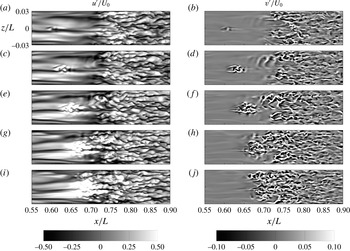
Temporal evolution of (left) $u^{\prime }$ and (right) $v^{\prime }$ contours at $y/L=0.850\times 10^{-3}$ : (a,b)  ${\it\tau}=0.042$ ; (c,d) ${\it\tau}=0.063$ ; (e,f) ${\it\tau}=0.084$ ; (g,h) ${\it\tau}=0.105$ ; (i,j) ${\it\tau}=0.126$ .

3.4. Visualisation of bypass transition and streak instability

The breakdown of the boundary layer to irregular motion is visualized in figure 14 by examining $u^{\prime }$ and $v^{\prime }$ contours in a $y$ – $z$ plane at $y/L=0.850\times 10^{-3}$ , which is about $0.5{\it\delta}^{\ast }$ above the test surface within the region shown, at time instances in the range ${\it\tau}=0.042{-}0.126$ . Two flow features are particularly prominent: a notable demarcation between turbulent and non-turbulent zones is observed in the $u^{\prime }$ and $v^{\prime }$ contours between $x/L=0.70$ and $x/L=0.75$ , while a small disturbance develops further upstream near $x/L=0.60$ and $z/L=0.00$ . The demarcation is relatively uniform in the spanwise ( $z$ ) direction, suggestive that transition at that location is abrupt and nearly homogeneous. The upstream disturbance, in contrast, is localized near a low-speed streak. By ${\it\tau}=0.063$ , this disturbance grows following the breakdown of the low-speed streak into smaller scale motions that grow in time and form a distinct and finite region of irregular motion that resembles a turbulent spot. By ${\it\tau}=0.084$ , the spot has enlarged and convected towards the turbulent zone, merging with it by about ${\it\tau}=0.105$ . The flow at ${\it\tau}=0.126$ shows that when the spot merges with the turbulent zone, the interface between the turbulent and non-turbulent zones abruptly shifts to the location of the upstream (trailing) edge of the spot, causing the interface between the turbulent and non-turbulent region to vary in time and in the spanwise direction with an amplitude of up to $0.1L$ .

The flow features in figure 14 suggest that at least two distinct transition processes occur in the flow. The transition process associated with the localized disturbance occurs through the gradual formation and growth of localized regions of turbulent flow through the breakdown of low-speed streaks; this process resembles the scenario observed by Jacobs & Durbin (Reference Jacobs and Durbin2001), Zaki & Durbin (Reference Zaki and Durbin2006), Schlatter et al. (Reference Schlatter, Brandt, de Lange and Henningson2008) and others in zero and adverse pressure gradient flows. The transition process associated with the abrupt demarcation in the $u^{\prime }$ and $v^{\prime }$ contours occurs through the rapid amplification of disturbances introduced from the free stream in the adverse pressure gradient region of the flow. The local inflectional boundary layer allows disturbances to rapidly amplify and trigger transition almost homogeneously across the span, bypassing the spatially distributed formation, growth and coalescence of discrete turbulent spots. The shape of the intermittency parameter in figure 9(b) supports this explanation of the transition process; if transition were accomplished wholly by the growth and coalescence of discrete turbulent spots, the intermittency parameter would trace the smooth ‘S’ curve proposed by Emmons (Reference Emmons1951). The abrupt trend observed in the intermittency distribution in figure 9(b) suggests that while discrete turbulent spot production following streak breakdown is present, the abrupt bypass process due to the high free stream turbulence and adverse pressure gradient conditions may be dominant.

The $v$ -velocity fluctuations in figure 14(b) give a clearer impression of the localized disturbances that accompany the breakdown of the low-speed streak and the small-scale motions that form within the resulting turbulent spot. The $v^{\prime }$ contours at ${\it\tau}=0.042$ shows that the disturbance consists primarily of a strong localized $-v^{\prime }$ motion (sweep) surrounded by weaker and more dispersed $+v^{\prime }$ motions (ejections). At subsequent time instances, the $v^{\prime }$ contours amplify and elongate in sync with the growing turbulent spot, and the spanwise edges of the spot appear to be terminated by ejections. These likely correspond to ejection of low momentum fluid along the sides of the spot, which numerous studies of isolated turbulent spots in laminar boundary layers have shown to contribute to the lateral growth of the spot (e.g. Schröder & Kompenhans Reference Schröder and Kompenhans2004).

Figure 15.

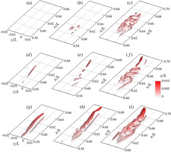
Transient breakdown of a low-speed streak illustrated through iso-contours of $u^{\prime }/U_{0}=-0.20$ (a,c,e,g) and $\unicode[STIX]{x1D64C}(L/U_{0})^{2}=5000$ (b,d,f,h). Iso-contours are coloured by $y/L$ and lines show selected samples of instantaneous vorticity lines: (a,b) ${\it\tau}=0.042$ , (c,d) ${\it\tau}=0.063$ , (e,f) ${\it\tau}=0.084$ , (g,h) ${\it\tau}=0.105$ .

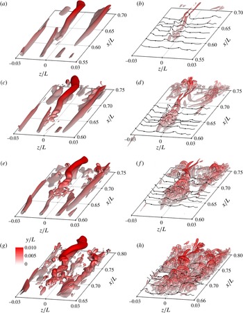
Before the nature of the streak breakdown is described, it is worthwhile to clarify the connection between the streak breakdown observed in figure 14 and the formation of coherent vortical structures in the transitional boundary layer. To do so, figure 15 re-plots the time instances of figure 14 using three-dimensional iso-contours of negative $u^{\prime }$ and the second invariant of the velocity gradient tensor, denoted $\unicode[STIX]{x1D64C}$ , defined as

where Einstein summation is implied over the indexed terms. The $\unicode[STIX]{x1D64C}$ property has been shown to improve the prominence of coherent vortices over the background vorticity (e.g. Jeong & Hussain Reference Jeong and Hussain1995). Instantaneous vorticity lines are also plotted to illustrate the correlation of the vorticity field with $\unicode[STIX]{x1D64C}$ ; for improved visibility of these lines, the $\unicode[STIX]{x1D64C}$ iso-contours are rendered semi-translucent. The $-u^{\prime }$ iso-contours at ${\it\tau}=0.042$ and 0.063 show that the perturbation of the low-speed streak under consideration (the one located near $z/L=0.00$ ) occurs near $x/L=0.625$ at a height of approximately $y/L=0.003{-}0.006$ (2–4 ${\it\delta}^{\ast }$ ). The $\unicode[STIX]{x1D64C}$ iso-contours indicate that the perturbations correspond to small hairpin vortices that extend from near the wall to about 0.003 $L$ (corresponding to approximately 2 ${\it\delta}^{\ast }$ ), the initial formation of which is discussed below. By ${\it\tau}=0.063$ , the hairpin vortices have spawned subsequent generations of vortices, both in the streamwise direction and along the spanwise edges of the spot so that by ${\it\tau}=0.084$ , 4–5 generations of hairpin vortices exist across the span of the spot and 6–7 generations of hairpin vortices exist between the spot’s leading and trailing edges. The ‘kinks’ in the vorticity lines outboard of the spot’s spanwise edges at ${\it\tau}=0.084$ and earlier instances indicate regions where ejection of fluid induced by the vortices within the spot have lifted the vorticity line outboard of the spot. As the uplifted portions of the vorticity lines are stretched by the mean shear, they strengthen and form new hairpin vortices along the spanwise edges of the spot, resulting in the noted increase in the number of hairpin vortices within the spot. By ${\it\tau}=0.105$ , the spot has convected close enough to the downstream turbulent zone that it becomes difficult to differentiate the vortical structures belonging to the spot from those that make up the turbulent zone.

Figure 16.

Multiple instances of low-speed streak breakdown illustrated through iso-contours of $u^{\prime }/U_{0}=-0.20$ (a,c,e) and $\unicode[STIX]{x1D64C}(L/U_{0})^{2}=5000$ (b,d,f). Iso-contours are coloured by $y/L$ : (a,b) ${\it\tau}=0.063$ , (c,d) ${\it\tau}=0.211$ , (e,f) ${\it\tau}=0.392$ .

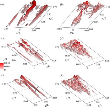
Returning to the $u^{\prime }$ iso-contours at ${\it\tau}=0.063$ in figure 15, it is evident that the wall-normal motions induced by the hairpin vortices within the growing turbulent spot correspond to the localized motions that are observed as the low-speed streak breaks into discrete packets of low-speed fluid. If the $u^{\prime }$ contours are analysed in an $x$ – $y$ plane that intersects the unstable streak, a symmetric streamwise grouping of low-speed fluid is observed, characteristic of the varicose secondary streak instability mode. Figure 15 shows that the coherent vortices that form following the roll-up of the low-speed streak initially have a streamwise periodic structure before they break into three-dimensional vortices. These observations indicate that the breakdown of the low-speed streak into small-scale vortices occurs by a three-dimensional process, as noted previously by Le Cunff & Bottaro (Reference Le Cunff and Bottaro1993), Andersson et al. (Reference Andersson, Brandt, Bottaro and Henningson2001), Cherubini et al. (Reference Cherubini, De Palma, Robinet and Bottaro2011), amongst others, in which a streamwise periodic accumulation of vorticity occurs within the shear layer surrounding the low-speed streak that results in the noted streamwise waviness of the streak. The streamwise accumulation of shear layer vorticity is driven by the development of the varicose mode of secondary streak instability. This is illustrated for multiple low-speed streaks in figure 16 by plotting two additional instances in time alongside the instance at ${\it\tau}=0.063$ from figure 15. In each instance, streamwise periodic waviness of the highlighted low-speed streak is observed, and while the amplitude of this waviness differs among the multiple instances, it is generally clear that the streamwise waviness coincides with the formation of three-dimensional structures. This observation of varicose secondary instability on selected low-speed streaks is consistent with the recent DNS study of Hack & Zaki (Reference Hack and Zaki2014) who noted that the dominant secondary instability mode for streaks in adverse pressure gradient boundary layers under high free stream turbulence is the varicose mode. They also note that threshold streak amplitudes for varicose instability in adverse pressure gradients is significantly lower than in zero pressure gradient boundary layers, and can be below 20 %, which is satisfied by the streak amplitudes of 24–28 % in the present study (figure 13).

Figure 17.

Transient evolution of vortical flow structures within the free stream turbulence, illustrated through iso-contours of $\unicode[STIX]{x1D64C}(L/U_{0})^{2}=500$ coloured by $y/L$ at: (a) ${\it\tau}=0.021$ and (b) ${\it\tau}=0.042$ .

Figure 18.

Interaction of a free stream vortical disturbance and a streamwise low velocity streak in the $z/L=-0.002$ plane. Contours are of $u^{\prime }/U_{0}$ and lines are $v^{\prime }/U_{0}=0.10$ (solid) and $v^{\prime }/U_{0}=-0.10$ (dashed): (a) ${\it\tau}=0.021$ ; (b) ${\it\tau}=0.032$ ; (c) ${\it\tau}=0.042$ ; (d)  ${\it\tau}=0.053$ ; (e) ${\it\tau}=0.063$ .

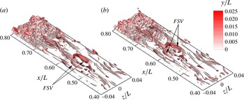
Brandt & de Lange (Reference Brandt and de Lange2008) and Hack & Zaki (Reference Hack and Zaki2014) attribute the development of the varicose mode to a localized instability of the strong shear layer that develops between high- and low-speed streaks when the high-speed streak is situated above the low-speed streak. Such a configuration may occur when low-speed streaks interact with discrete vortical structures in the free stream turbulence. Figure 17 illustrates these structures by plotting normalized iso-contours of $\unicode[STIX]{x1D64C}$ . The threshold for the iso-contours ( $\unicode[STIX]{x1D64C}(L/U_{0})^{2}=500$ ) is one-tenth of the value used in figure 15, which allows the weaker coherent structures in the free stream turbulence to be visualized. The structures labelled FSV (free stream vortex) indicate discrete vortical disturbances (eddies) located at a wall-normal distance of about $y/L=0.020{-}0.025$ or 16–20 ${\it\delta}^{\ast }$ . 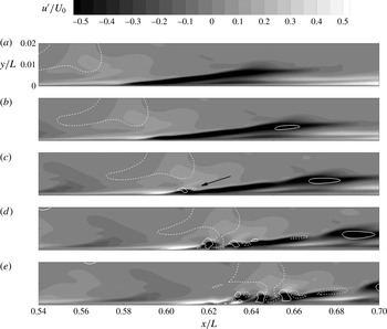The anisotropic shape of the eddies is due to the strong free stream acceleration, which stretches them in the streamwise direction as they convect through the favourable pressure gradient region of the flow. The interaction of the free stream vortical disturbances with the low-speed streak is illustrated in figure 18 by plotting $u^{\prime }$ contours and $v^{\prime }/U_{0}=\pm 0.1$ lines in an $x$ – $y$ plane at $z/L=-0.002$ , which roughly intersects the middle of the low-speed streak. The dashed $-v^{\prime }$ contours prevailing in the free stream upstream of the low-speed streak at ${\it\tau}=0.021$ are sweep motions induced by the free stream eddies. The sweep introduces high momentum fluid into the boundary layer that results in the formation of a high-speed streak beneath the eddy in the wake of the low-speed streak. Because the low-speed streak moves slower than the local mean flow, the eddy and the high-speed streak it creates gradually overtake the upstream edge of the low-speed streak. This is evident at ${\it\tau}=0.032$ in figure 18 where the high-speed streak collides with and begins to convect above the upstream edge of the low-speed streak. As the sweep events caused by the free stream eddy continually energize the high-speed streak, its amplitude increases and a thin region of very high shear stress develops at the interface between the high- and low-speed streaks. This shear layer is unstable to high-frequency disturbances via an inviscid instability mode due to its inflectional wall-normal velocity profile so that by ${\it\tau}=0.042$ , it begins to roll-up into discrete, spanwise-oriented vortices. According to Helmholtz’s vorticity laws, the rolled-up spanwise vortices must remain continuously connected to the spanwise vorticity that exists along the test surface wall, and because the interfacial shear layer lies relatively far from the wall, the rolled-up segments are convected faster than the ends that remain connected to the near wall vorticity. The resulting stretching gives the rolled-up vortex its hairpin shape seen at ${\it\tau}=0.042$ in figure 15. Small-scale wall-normal motions induced by the hairpin vortices, indicated in figure 18 by the arrow at ${\it\tau}=0.042$ , create a streamwise grouping of low-speed fluid, visible at ${\it\tau}=0.053$ and 0.063, and ultimately result in the breakdown of the low-speed streak into a turbulent spot.

The flow development shown in figure 18 strongly suggests that the three-dimensional roll-up and breakdown of low-speed streaks via varicose secondary instability coincides with strong $-v^{\prime }$ motions caused by eddies in the free stream turbulence above the streaks. When streaks at other times and spatial locations are analysed, it is consistently observed that low-speed streaks that are not below a large $-v^{\prime }$ eddy in the free stream turbulence do not break down into a turbulent spot as in figure 18. Instead, they maintain their coherence until they either convect into the downstream turbulent zone or are entrained by a neighbouring turbulent spot. This implies that a discrete free stream disturbance is required for streak breakdown to occur. Such a requirement is also observed by Liu, Zaki & Durbin (Reference Liu, Zaki and Durbin2008) in a DNS in which discrete and continuous modes of the Orr–Sommerfeld equation are forced in a transitional zero pressure gradient boundary layer. The discrete modes correspond to vortical disturbances within the flow and the continuous modes correspond to high- and low-speed streaks. Neither mode is sufficient to cause transition alone, as the discrete modes in isolation tend to be damped, but their mutual interaction results in the formation of a pattern of ${\rm\Lambda}$ -shaped structures with a wavelength that is smaller than the secondary instability of the discrete Orr–Sommerfeld modes, which is qualitatively similar to the closely spaced hairpin vortices observed in the present study. Furthermore, the DNS study of Zaki & Durbin (Reference Zaki and Durbin2006) indicates that the local adverse pressure gradient in the present study enhances the coupling between the free stream vortical disturbances and the boundary layer streaks. Simulations of Brandt & de Lange (Reference Brandt and de Lange2008) and Schlatter et al. (Reference Schlatter, Brandt, de Lange and Henningson2008) and particle image velocimetry measurements of Nolan & Walsh (Reference Nolan and Walsh2012) also corroborate the present observations that streak breakdown originates in the three-dimensional instability of the interfacial shear layer between the head of an oncoming high-speed streak and the tail of a downstream low-speed streak.

The present results aid in generalizing the findings of the above studies owing to the much stronger adverse pressure gradient conditions of the present study. As a comparison, the adverse pressure gradient imposed by Hack & Zaki (Reference Hack and Zaki2014) corresponds to a Hartree parameter of ${\it\beta}_{H}=-0.14$ , which is much lower than the critical value of about ${\it\beta}_{H}=-0.199$ required for boundary layer separation under low free stream turbulence. In contrast, if the pressure gradient of the present study occurs under low free stream turbulence, flow separation occurs shortly downstream of the suction peak (Brinkerhoff & Yaras Reference Brinkerhoff and Yaras2011). The present study demonstrates that even in strongly adverse pressure gradients, varicose secondary streak instability is still observed if the streak is accompanied by an appropriate free stream disturbance. If the requisite free stream disturbance is not present, transition proceeds by an abrupt amplification of free stream disturbances within the inflectional boundary layer resulting in a nearly homogeneous breakdown across the span without the distributed growth of turbulent spots.

3.5. Growth mechanism of turbulent spots

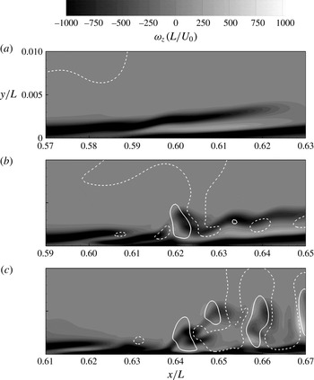
The growth mechanism of the turbulent spot that forms following the development of varicose secondary instability of a low-speed streak is now considered. It was noted earlier that the mean shear shelters the boundary layer from high-frequency free stream disturbances so that only low-frequency disturbances are able to penetrate deep into the boundary layer. However, once the shear layer surrounding a low-speed streak rolls-up, the instantaneous shear layer becomes spatially discontiguous so that high-frequency disturbances can now penetrate from the free stream into the boundary layer. This is illustrated in figure 19 by plotting $v^{\prime }$ lines and the instantaneous spanwise vorticity ( ${\it\omega}_{z}$ ) contours in the rolled-up portions of the shear layer from figure 18. To highlight the temporal development of the shear layer, the axial coordinate is shifted to keep the convecting low-speed streak in the centre of the plotted data, and the wall-normal coordinate is stretched by a factor of two. The contiguous shear layer located away from the wall at ${\it\tau}=0.032$ corresponds to the strong interfacial shear layer created between the high- and low-speed streaks. Because of the shear sheltering effect, free stream vortical disturbances are not able to penetrate through this shear layer, as indicated by the $v^{\prime }$ contour lines. However, as the interfacial shear layer rolls-up, as at ${\it\tau}=0.053$ , it is no longer contiguous and free stream vortical disturbances are able to penetrate through the shear layer towards the wall, coupling with the small-scale $v^{\prime }$ motions that are induced by the hairpin vortices. In three dimensions, this corresponds to sweep motions from the free stream disturbances penetrating between the hairpin vortices surrounding the low-speed streak. At ${\it\tau}=0.074$ it is evident that the sweep motions penetrate far into the boundary layer, reaching very near the wall, where they energize the small-scale vortical structures and accelerate the growth of the turbulent spot.

Figure 19.

Temporal evolution of instantaneous spanwise shear through ${\it\omega}_{z}(L/U_{0})$ contours in the $z/L=-0.002$ plane: (a) ${\it\tau}=0.032$ ; (b) ${\it\tau}=0.053$ ; (c) ${\it\tau}=0.074$ .

Further clarity of the physical role of the sweep motions induced by free stream disturbances in bypass transition is obtained by examining the equation governing the inviscid transport of instantaneous vorticity, ${\it\omega}_{i}$ :

Einstein summation is implied over the indexed terms, and $u_{i}$ is the instantaneous velocity. The terms on the right-hand side of (3.3) represent the convective transport of ${\it\omega}_{i}$ and its production by stretching and tilting, respectively. Figure 20 plots iso-contours of $(\partial {\it\omega}_{i}/\partial t)(L/U_{0})^{2}$ at three instances in time covering the time range shown in figure 18 to illustrate the spatial and temporal evolution of the vorticity field around the low-speed streak as it breaks down. At ${\it\tau}=0.021$ , the vorticity growth rate occurs predominantly in the $z$ component through a spatially coherent region of high $\partial {\it\omega}_{z}/\partial t$ that coincides with the location of the low-speed streak. By ${\it\tau}=0.042$ , the coherent region of high $\partial {\it\omega}_{z}/\partial t$ has begun to break into discrete regions that coincide with the locations where the low-speed streak rolls-up into three-dimensional vortices. Noting that the regions of high $\partial {\it\omega}_{z}/\partial t$ occur only at the site of the rolled-up vortices provides further evidence that the streak breakdown is indeed initiated by instability of the interfacial shear layer between the low- and high-speed streaks. Substantial regions of large $\partial {\it\omega}_{x}/\partial t$ and $\partial {\it\omega}_{y}/\partial t$ are not observed until ${\it\tau}=0.063$ , well after the roll-up of the low-speed streak has completed. This appears to support the argument given above that the low-speed streak must roll-up before small-scale disturbances from the free stream are able to penetrate through the shear layer and produce small-scale vortices near the wall.

Figure 20.

Evolution of the instantaneous vorticity field during the breakdown of a low-speed streak. Iso-contours are (a–c) $\partial {\it\omega}_{x}/\partial t$ , (d–f) $\partial {\it\omega}_{y}/\partial t$ , and (g–i) $\partial {\it\omega}_{z}/\partial t$ . The iso-contour levels are $(\partial {\it\omega}_{i}/\partial t)(L/U_{0})^{2}=1.2\times 10^{5}$ and are coloured by $y/L$ : (a,d,g) ${\it\tau}=0.021$ ; (b,e,h) ${\it\tau}=0.042$ ; (c,f,i) ${\it\tau}=0.063$ .

Figure 21.

Contour levels of the budgets of instantaneous vorticity equation (3.3) in the $z/L=-0.002$ plane at ${\it\tau}=0.053$ : (a) $\text{D}{\it\omega}_{x}/\text{D}t$ , ${\it\omega}_{x}$ -stretching,  ${\it\omega}_{x}$ -tilting; (b) $\text{D}{\it\omega}_{y}/\text{D}t$ , ${\it\omega}_{y}$ -stretching,  ${\it\omega}_{y}$ -tilting; (c) $\text{D}{\it\omega}_{z}/\text{D}t$ , ${\it\omega}_{z}$ -stretching,  ${\it\omega}_{z}$ -tilting. Contours are normalized by $(U_{0}/L)^{2}$ .

The connection between the vorticity growth rates and the near wall fluctuating motions is obtained by analysing the budgets of (3.3). Figure 21 plots the budgets normalized by $(U_{0}/L)^{2}$ at time ${\it\tau}=0.053$ in a $x$ – $y$ plane at $z/L=-0.002$ that roughly intersects the middle of the iso-contours plotted in figure 20. Vorticity production due to vortex stretching ( ${\it\omega}_{i}\partial u_{i}/\partial x_{i}$ ) and vortex tilting ( ${\it\omega}_{j}\partial u_{i}/\partial x_{j}$ , $i\neq j$ ) are plotted separately to distinguish between the two processes. Consistent with figure 20, the budgets indicate that the temporal variation of vorticity is dominated by growth in the ${\it\omega}_{z}$ component. Furthermore, the $\text{D}{\it\omega}_{z}/\text{D}t$ contours appear to correlate primarily with the ${\it\omega}_{z}$ -stretching process, which suggests that growth of vorticity surrounding the low-speed streak is primarily due to the stretching of existing ${\it\omega}_{z}$ by the local fluctuating velocity field. The nature of the fluctuating velocity field occurring in the near wall region below the low-speed streak is shown in figure 22(a). Vectors illustrating the fluctuating wall-normal and spanwise velocity components are plotted in the $y$ – $z$ plane at $x/L=0.625$ , which intersects the rolled-up portion of the low-speed streak at time ${\it\tau}=0.053$ . The vectors near the wall at around $z/L\approx -0.003$ illustrate the strong sweep motions that are induced by the free stream vortical disturbances as they penetrate through the rolled-up shear layer towards the wall. The vectors show that as the sweep motions approach the wall, they are turned in the spanwise direction by the solid surface, generating strong local $w^{\prime }$ motions, and hence the large $\partial w/\partial z$ strain rates that are required for the ${\it\omega}_{z}$ -stretching process.

Figure 22.

Contours of (a) $(\partial v/\partial x)L/U_{0}$ , (b) $(\partial w/\partial x)L/U_{0}$ , (c) $(\partial v/\partial z)L/U_{0}$ , and (d) $(\partial w/\partial y)L/U_{0}$ in the $x/L=0.625$ plane at ${\it\tau}=0.053$ . Vectors in (a) illustrate the in-plane $v^{\prime }$ and $w^{\prime }$ motions, and lines in (b) are $v^{\prime }/U_{0}=0.10$ (solid) and $v^{\prime }/U_{0}=-0.10$ (dashed).

Although the growth rates of ${\it\omega}_{x}$ and ${\it\omega}_{y}$ in the near wall region below the low-speed streak are lower than the growth rate of ${\it\omega}_{z}$ , the growth of the ${\it\omega}_{x}$ and ${\it\omega}_{y}$ vorticity components contribute to the loss of symmetry of the flow during breakdown into small-scale vortices (figure 20), and thus merit discussion. Figure 21 shows that the $\text{D}{\it\omega}_{x}/\text{D}t$ and $\text{D}{\it\omega}_{y}/\text{D}t$ contours correlate most closely with their respective tilting terms, which can be expanded in terms of the instantaneous strain rates as:

The strain rates in the above equations are plotted as contours in figure 22. The $\partial u/\partial y$ and $\partial u/\partial z$ terms are not plotted because they are predominantly formed by the background flow – $\partial u/\partial y$ corresponds to the mean shear and $\partial u/\partial z$ corresponds to the longitudinal streaks – while the remaining strain rates are formed by the free stream disturbances following the breakdown of the low-speed streak. The most obvious contributor to the vortex tilting process is the $\partial w/\partial y$ strain rate shown in figure 22(c). In light of the fluctuating velocity field shown in figure 22(a), it appears that this strain rate – like the $\partial w/\partial z$ strain rate in the ${\it\omega}_{z}$ -stretching term – is produced when sweep motions induced by the free stream vortical disturbances are turned in the spanwise direction by the presence of the wall. These observations suggest that sweep motions produced by the coherent structures in the free stream turbulence activate vorticity production processes coinciding with the roll-up of a low-speed streak and result in the production of small-scale vortices. The production of these small-scale vortices drives the enlargement of the turbulent flow region and ultimately results in transition to fully turbulent flow.