1. Introduction
Resolvent analysis is an operator-theoretic modal decomposition method, providing a promising tool to investigate the prominent mechanisms underpinning the dynamics of turbulence (McKeon & Sharma Reference McKeon and Sharma2010; Taira et al. Reference Taira, Brunton, Dawson, Rowley, Colonius, McKeon, Schmidt, Gordeyev, Theofilis and Ukeiley2017; Jovanović Reference Jovanović2021). In the framework of resolvent analysis, a linear dynamical system is obtained by linearising the Navier–Stokes equations around a steady base flow, with a resolvent operator relating the forcing input to the response output. The resolvent operator is comprised of the time-averaged variables, which are usually assumed to be known a priori. The forcing input represents the nonlinear advection terms in the governing equations, and the response output includes velocities, density and temperature in the regime of compressible turbulent flows (Bae, Dawson & McKeon Reference Bae, Dawson and McKeon2020). These nonlinear terms in the input can be obtained with high-fidelity numerical simulations, but the computational cost is prohibitive (Gupta et al. Reference Gupta, Madhusudanan, Wan, Illingworth and Juniper2021) especially in compressible turbulent boundary layers with strong heat transfer at the wall. Due to the variation of thermodynamic properties and the coupling between aerodynamic and thermodynamic structures, high-order nonlinear terms become more complicated and, hence, their modelling more challenging (Wenzel, Gibis & Kloker Reference Wenzel, Gibis and Kloker2022). Therefore, how to deal with the nonlinear forcing input is one of the crucial issues in the resolvent-based estimation of compressible turbulent boundary layers.
McKeon & Sharma (Reference McKeon and Sharma2010) treated the entire nonlinear term as an unknown endogenous stimulus. The qualitative characteristics of turbulent motions are fully conveyed by the resolvent operator. They performed singular value decomposition of the resolvent operator in incompressible pipe flows, so that responses to the endogenous stimulus are ranked at a specific wavenumber and frequency pair. High-gain input (forcing) and output (response) modes are highlighted and used to reproduce the predominant turbulent structures. This approach has been used widely to identify and model the coherent structures in wall-bounded turbulent flows. Sharma & McKeon (Reference Sharma and McKeon2013) reconstructed the coherent structures in turbulent pipe flows from a linear superposition of optimal response modes at representative wavenumber combinations, forming a low-rank description of coherent structures. With the resolvent decomposition, a reduced-order model of the unsteady cavity flow was constructed based on the time-averaged flow field (Gómez et al. Reference Gómez, Blackburn, Rudman, Sharma and McKeon2016). In the study of Abreu et al. (Reference Abreu, Cavalieri, Schlatter, Vinuesa and Henningson2020), the performance of resolvent analysis in modelling near-wall coherent structures was compared with that of spectral proper orthogonal decomposition (SPOD). They observed a good alignment between the resolvent and SPOD modes in channel flows, especially under the condition where the optimal resolvent gain is dominant. Fan, Chen & Li (Reference Fan, Chen and Li2024a ) proposed a modelling framework, based on low-rank resolvent modes and machine learning, to predict the turbulent energy in incompressible channel flows, where the optimal response modes serve as the basis functions and the projection coefficients of the forcing modes onto the true nonlinear terms are obtained through data-driven neural networks. Based on the low-rank resolvent analysis, Luhar et al. (Reference Luhar, Sharma and McKeon2014, 2015) investigated the impacts of opposition control and compliant walls on the response modes in fully developed pipe and channel flows, by incorporating the flow-control effects into the resolvent operator. More recently, extensions of the resolvent analysis to compressible forms have been developed by Dawson, McKeon & Saxton-Fox (Reference Dawson, McKeon and Saxton-Fox2018) and Dawson & McKeon (Reference Dawson and McKeon2019). In supersonic turbulent boundary layers, the reduced-order approximation of the compressible resolvent operator highlighted two distinct regions in the wavenumber space (Bae et al. Reference Bae, Dawson and McKeon2020): (i) the relatively subsonic region, where the low-rank behaviour of the resolvent operator was observed in alignment with the incompressible counterpart; and (ii) the relatively supersonic region, where the resonant amplification appears in the leading response mode. Mechanisms that are responsible for the energy amplification in the relatively subsonic and supersonic modes were then identified with Helmholtz decomposition applied to the forcing terms in the momentum equations (Madhusudanan & McKeon Reference Madhusudanan and McKeon2022; Chen et al. Reference Chen, Cheng, Gan and Fu2023). In the study of Fan, Li & Sandberg (Reference Fan, Li and Sandberg2023), the low-rank nature of the resolvent operator in compressible turbulent boundary layers was investigated, revealing the energy distribution and identifying streaks and hairpin vortices under the different conditions of isothermal walls. In general, this classical approach bypasses the high-cost computation or specific modelling of the nonlinear forcing terms. The literature has focused on investigating the turbulent characteristics inherent in the linear resolvent operator that is solely dependent on the mean flow state. However, this treatment actually neglects the role of the nonlinear process, hence losing important information in terms of the turbulence cycle.
An alternative approach is to model part of the nonlinear forcing and to treat the remainder with further assumptions or simplifications. One of the most commonly used techniques is to add appropriate eddy viscosity to model the oscillation of Reynolds stresses associated with the passage of disturbances and, consequently, reformulate the resolvent operator. In incompressible channel flows, results showed that the Cess eddy-viscosity model (Cess Reference Cess1958; Reynolds & Hussain Reference Reynolds and Hussain1972) can efficiently improve the capability of resolvent modes in predictions of the instantaneous velocity fields (Illingworth, Monty & Marusic Reference Illingworth, Monty and Marusic2018; Madhusudanan, Illingworth & Marusic Reference Madhusudanan, Illingworth and Marusic2019) and spatio–temporal power spectral densities(PSDs) (Morra et al. Reference Morra, Semeraro, Henningson and Cossu2019; Symon, Illingworth & Marusic Reference Symon, Illingworth and Marusic2020), especially for the high-energy-containing scales. Pickering et al. (Reference Pickering, Rigas, Schmidt, Sipp and Colonius2021) examined four models for the eddy-viscosity field in turbulent jets, and obtained an optimal one that aligns the corresponding resolvent modes to measured SPOD modes. Furthermore, in the regime of compressible turbulent boundary layers, Fan et al. (Reference Fan, Kozul, Li and Sandberg2024b ) proposed two eddy-viscosity models to improve the low-rank approximation of resolvent analysis, i.e. (i) a modified Cess eddy-viscosity model coupling the compressibility transformation and outer-layer correction, and (ii) a new semi-empirical eddy-viscosity model based on a fitting law of total shear stress and mixing-length hypothesis. To gain further insight into the underlying mechanism of eddy-viscosity effects, Symon, Illingworth & Marusic (Reference Symon, Illingworth and Marusic2021) analysed the energy budgets for optimal resolvent modes, including production, viscous dissipation and nonlinear transfer. They reported that the addition of eddy viscosity provides additional turbulent dissipation to well reproduce the actual nonlinear transfer from large-scale to small-scale motions in channel flows (Symon et al. Reference Symon, Illingworth and Marusic2021Reference Symon, Madhusudanan, Illingworth and Marusic2023), although the quantitative accuracy is constrained within the most energetic modes. As for the remaining part of the nonlinear term, Gupta et al. (Reference Gupta, Madhusudanan, Wan, Illingworth and Juniper2021) assumed it to be proportional to the eddy dissipation term that is modelled with a scale-dependent Cess eddy viscosity, so that the energy transfer modelled by the eddy dissipation and stochastic forcing can balance each other at most wall-normal locations. With this method, they reported reasonably good performance in the estimation of large-scale fluctuations in incompressible channel flows. Similar to the study in McKeon & Sharma (Reference McKeon and Sharma2010), these eddy-viscosity-improved resolvent analyses still focus on the investigation of the resolvent operator, and do not require the a priori knowledge of the turbulent fluctuations. Although the resolvent operator with/without eddy viscosity is able to describe the input–output relationship between the flow instantaneous states and the nonlinear feedback, the quantitative effects of the nonlinear forcing terms are missed, hence leading to intrinsic constraints to these methods (Nogueira et al. Reference Nogueira, Morra, Martini, Cavalieri and Henningson2021).
Instead of ignoring the nonlinear forcing or simply assuming it to be stochastic, estimations of the forcing statistics have been conducted to enable the resolvent-based predictions of turbulence, on the basis of limited known flow information (Zare, Jovanović & Georgiou Reference Zare, Jovanović and Georgiou2017; Towne, Lozano-Duran & Yang Reference Towne, Lozano-Duran and Yang2020; Holford, Lee & Hwang Reference Holford, Lee and Hwang2023). However, with the aim being predicting turbulent statistics, e.g. the spectra of velocities, they did not examine the characteristics of the estimated forcing or compare it to the real forcing. It means that the role of the estimated nonlinearity in the turbulence cycle has not been confirmed. To fully recover the coherent flow fields using linear resolvent analysis, Towne (Reference Towne2016) pointed out that appropriate characterisation and parameterisation of the nonlinear forcing input is necessary. To this end, access to the actual nonlinear forcing term can be of great benefit, supporting the development and validation of turbulence modelling techniques (Beneddine et al. Reference Beneddine, Sipp, Arnault, Dandois and Lesshafft2016). Morra et al. (Reference Morra, Nogueira, Cavalieri and Henningson2021) calculated the nonlinear forcing term through direct numerical simulations (DNS) of incompressible turbulent channel flows at two friction Reynolds numbers. The influence of the forcing (input) statistics on the amplified response (output) was investigated, by decomposing the cross-spectral densities (CSDs) of the forcing term into solenoidal and non-solenoidal parts. Using real statistics from DNS of minimal turbulent Couette flow, a quantitative relation between the CSDs of the output velocity and input forcing has been evaluated and confirmed (Nogueira et al. Reference Nogueira, Morra, Martini, Cavalieri and Henningson2021), so as to identify the most relevant forcing components in the self-sustaining turbulence cycle. As for the characteristics and modelling of the nonlinear forcing statistics in compressible turbulence, few studies can be found in the open literature, to the best of the authors’ knowledge.
This work ultimately seeks to predict the turbulent fluctuations (output of the resolvent formulation) in compressible turbulent boundary layers. Hence, the distribution of forcing statistics (input to the resolvent formulation) and their quantitative influence on the output is a focus of this paper. To this end, the nonlinear forcing terms are calculated using DNS data of compressible turbulent boundary layers under adiabatic and cold-wall conditions. The remainder of the paper is structured as follows. Section 2 gives the resolvent formulations for compressible turbulent boundary layers, especially exhibiting the turbulent fluctuations as a response output of the nonlinear forcing. The DNS dataset of two compressible turbulent boundary layers with and without wall cooling is introduced in § 3. In § 4 the nonlinear forcing is quantified to investigate its spectral characteristics and the influence on responses in detail. Based on the findings herein, estimations of the statistical spectral densities of flow perturbations are conducted with the modelled CSD of forcing. Concluding remarks are given in § 5.
2. Resolvent formulation
The fully developed compressible turbulent boundary layer is assumed to be a quasi-parallel flow, i.e. the effect of the streamwise development is ignored. This assumption is reasonable since the base flow of a zero-pressure-gradient turbulent boundary layer evolves over a slower viscous time scale than the convective processes of fluctuations (Bae et al. Reference Bae, Dawson and McKeon2020), which suggests that the variation of the mean flow variables in the streamwise direction is very small compared with the rapid turbulent fluctuations. In this sense, the state variables
 $\boldsymbol{q}= [u_{1}, u_{2}, u_{3}, \rho , T ]^{\top }$
can be Fourier transformed in the streamwise, spanwise and temporal directions, that is,
 \begin{equation} \boldsymbol{q}\!\left (x_{1}, x_{2}, x_{3}, t\right )=\iiint _{-\infty }^{\infty } \hat {\boldsymbol{q}}\!\left (x_{2} ; \kappa _{1}, \kappa _{3}, \omega \right ) \mathrm{e}^{\mathrm{i}\!\left (\kappa _{1} x_{1}+\kappa _{3} x_{3}-\omega t\right )} \mathrm{d} \kappa _{1} \mathrm{d} \kappa _{3} \mathrm{d} \omega , \end{equation}
where
 $t$
is time,
 $x_k$
(
 $k$
= 1, 2, 3) represent the streamwise, wall-normal and spanwise directions,
 $u_k$
are the corresponding velocity components,
 $\rho$
is density and
 $T$
is temperature. Note that the lengths are non-dimensionalised by the
 $99\,\%$
boundary-layer thickness
 $\delta _{99}$
, and the other variables are non-dimensionalised by their respective free-stream quantities. Here
 $\hat {(\cdot )}$
denotes the Fourier-transformed variable,
 $\top$
denotes the matrix transpose,
 $\kappa _1$
and
 $\kappa _3$
are the streamwise and spanwise wavenumbers,
 $\omega$
is the temporal frequency and
 $\mathrm{i}=\sqrt {-1}$
. The speed of the streamwise wave is defined by
 $c = \omega /k_1$
.
Substituting the Fourier transform (2.1) into the Navier–Stokes equations (as expressed in Appendix A), we obtain the linearised governing equations in the Fourier domain as
 \begin{equation} \left [-\mathrm{i} \omega \boldsymbol{I}+\boldsymbol{L}\!\left (\kappa _{1}, \kappa _{3}, \omega \right )\right ]\hat {\boldsymbol{q}}\!\left (x_{2} ; \kappa _{1}, \kappa _{3}, \omega \right )=\,\hat {\boldsymbol{\!f}}\!\left (x_{2} ; \kappa _{1}, \kappa _{3}, \omega \right )\!, \end{equation}
where
 $(\kappa _1, \kappa _3, \omega )\ne (0,0,0)$
,
 $\boldsymbol{I}$
is the identity matrix and
 $\,\hat {\boldsymbol{\!f}}$
is termed the forcing, containing all the high-order nonlinear contributions in the Navier–Stokes equations. The expression of
 $\boldsymbol{f}$
is given in Appendix A, and the expression of
 $L$
can be found in Fan et al. (Reference Fan, Li and Sandberg2023).
Hence, the flow states may manifest as a response to the nonlinear forcing in an input–output system, i.e.
 \begin{equation} \hat {\boldsymbol{q}}\!\left (x_{2} ; \kappa _{1}, \kappa _{3}, \omega \right )=\boldsymbol{H}\!\left (\kappa _{1}, \kappa _{3}, \omega \right ) \,\hat {\boldsymbol{\!f}}\!\left (x_{2} ; \kappa _{1}, \kappa _{3}, \omega \right )\!, \end{equation}
with the resolvent operator
 $\boldsymbol{H} (\kappa _{1}, \kappa _{3}, \omega )= (-\mathrm{i} \omega \boldsymbol{I}+\boldsymbol{L} (\kappa _{1}, \kappa _{3}, \omega ) )^{-1}$
. Consequently, the CSDs of forcing (
 ${\boldsymbol{S}}_{{\!\boldsymbol{f\!f}}}$
) and response (
 ${\boldsymbol{S}}_{{\boldsymbol{qq}}}$
) are correlated by
 \begin{equation} {\boldsymbol{S}}_{{\boldsymbol{qq}}}\!\left (x_{2}, x_{2}'; \kappa _{1}, \kappa _{3}, \omega \right )=\boldsymbol{H}\!\left (\kappa _{1}, \kappa _{3}, \omega \right ){\boldsymbol{S}}_{{\!\boldsymbol{f\!f}}}\!\left (x_{2}, x_{2}' ; \kappa _{1}, \kappa _{3}, \omega \right )\boldsymbol{H}^\dagger \!\left (\kappa _{1}, \kappa _{3}, \omega \right )\!, \end{equation}
where
 ${\boldsymbol{S}}_{{\boldsymbol{qq}}}= \hat {\boldsymbol{q}}\hat {\boldsymbol{q}}^\dagger$
and
 ${\boldsymbol{S}}_{{\!\boldsymbol{f\!f}}}= \,\hat {\boldsymbol{\!f}}\!\hat {\boldsymbol{\!f}}^\dagger$
. The superscript
 $\dagger$
denotes the complex conjugate transpose.
In the case where the forcing is assumed to be stochastic white noise, i.e.
 ${\boldsymbol{S}}_{{\!\boldsymbol{f\!f}}}=\boldsymbol{I}$
, the response can be easily obtained by
 ${\boldsymbol{S}}_{{\boldsymbol{qq}}}=\boldsymbol{H}\!\boldsymbol{H}^\dagger$
. However, this assumption is far from the real physics in turbulence, leading to unsatisfactory predictive performance in numerous previous studies (Morra et al. Reference Morra, Semeraro, Henningson and Cossu2019; Nogueira et al. Reference Nogueira, Morra, Martini, Cavalieri and Henningson2021; Symon et al. Reference Symon, Illingworth and Marusic2021). Hence, to estimate the energy distribution of response (
 ${\boldsymbol{S}}_{{\boldsymbol{qq}}}$
), appropriate modelling approaches/implications of the forcing CSD (
 ${\boldsymbol{S}}_{{\!\boldsymbol{f\!f}}}$
) are of interest. To this end, the statistical characteristics of
 ${\boldsymbol{S}}_{{\!\boldsymbol{f\!f}}}$
and the effects of its subcomponents on
 ${\boldsymbol{S}}_{{\boldsymbol{qq}}}$
will be investigated in the following sections.
3. Direct numerical simulation databases of compressible turbulent boundary layers
Two DNSs of compressible turbulent boundary layers were performed at a free-stream Mach number of
 $M_\infty = 5.86$
. A well-validated finite differencing solver, STREAmS (Supersonic TuRbulEnt Accelerated navier–stokes Solver) (Bernardini et al. Reference Bernardini, Modesti, Salvadore and Pirozzoli2021), was used. Two wall thermal conditions were considered, i.e. the adiabatic- and cold-wall condition defined by the wall-to-recovery temperature ratio
 $T_w^*/T_r^*=$
1.0 and 0.25, respectively. The superscript
 $*$
denotes dimensional values, the subscript
 $w$
denotes variables at the wall and
 $T_r^*$
is the nominal recovery temperature defined by
 $T_r^* = T_\infty ^* [1+r(\gamma -1)M_\infty ^2/2]$
, where
 $r=0.89$
and
 $\gamma$
is the specific heat ratio. Flow stations where the friction Reynolds number
 ${Re}_\tau = \rho _w^* u_\tau ^* \delta _{99}^*/\mu _w^* \approx 420$
(with
 $u_\tau ^*$
being the friction velocity and
 $\mu _w^*$
the wall dynamic viscosity) were selected for statistics sampling in this study. Additional boundary-layer properties, including the inflow Reynolds number
 ${Re}_{\delta _{in}}$
, the momentum-thickness-based Reynolds number with the free-stream viscosity
 ${Re}_\theta$
and with the wall viscosity
 ${Re}_{\delta 2}$
, and the shape factor
 $H_{12}$
are given in table 1. Here
 ${Re}_{\delta _{in}}=\rho _\infty ^* u_\infty ^* \delta _{in}^*/\mu _\infty ^*$
,
 ${Re}_\theta = \rho _\infty ^* u_\infty ^* \theta ^* /\mu _\infty ^*$
,
 ${Re}_{\delta 2}= \rho _\infty ^* u_\infty ^* \theta ^* /\mu _w^*$
and
 $H_{12} = \delta ^{\star *}/\theta ^*$
, where
 $\delta _{in}^*$
denotes the
 $99\,\%$
boundary-layer thickness at the inflow station,
 $\theta ^*$
represents the momentum thickness,
 $\delta ^{\star *}$
is the displacement thickness and the subscript
 $\infty$
denotes free-stream variables. Detailed settings and grid resolutions for the DNS can be retrieved from Fan & Li (Reference Fan and Li2023), and the convergence of the flow statistics has been carefully checked and validated in comparison to the corresponding DNS cases reported in previous papers (Zhang, Duan & Choudhari Reference Zhang, Duan and Choudhari2018; Huang, Duan & Choudhari Reference Huang, Duan and Choudhari2022).
Flow conditions of the turbulent boundary layers.

4. Results and discussion
In this section we aim to investigate the characteristics of the forcing and reveal its role in yielding the response, which consequently facilitates the modelling of the nonlinear forcing term in the input–output framework. Firstly, the spectral densities of the real nonlinear forcing with and without incorporating the eddy viscosity are examined. Secondly, the contribution of different forcing components to flow responses is quantified by means of reduced-order analysis, matrix decomposition and adopting the assumption of forcing decorrelation in space and components, so as to measure the relative importance of each forcing component in generating turbulence. At last, based on the current findings, a more representative model of the forcing input is proposed to estimate the statistical spectral densities of flow perturbations.
4.1. Characteristics of the forcing statistics
4.1.1. Spectral density of forcing
To investigate the statistics of the forcing, two representative space scales are selected at local energy peaks to characterise the near-wall cycle and outer-layer motions, following our previous study (Fan et al. Reference Fan, Kozul, Li and Sandberg2024b
). In the adiabatic turbulent boundary layer, the two representative scales are
 $(\lambda _1^+,\lambda _3^+)=(465,96)$
and
 $(\lambda _1,\lambda _3)=(2.85,1.06)$
, corresponding to the peak of turbulent energy in the inner and outer regions, respectively (Fan & Li Reference Fan and Li2023). The superscript
 $+$
denotes the normalisation by wall units, i.e. the velocity is scaled by
 $u_\tau ^*$
and the length by
 $\delta _\nu ^*=\mu _w^*/\rho _w^*u_\tau ^*$
. In the present paper, this classical inner scaling is applied so as to ensure the
 $x_2^+$
range from the wall surface to the boundary-layer height is the same for the current two turbulent boundary layers.
Power spectral density of the (a) real streamwise forcing extracted from DNS and (b) optimal forcing mode at
 $(\lambda _1^+,\lambda _3^+)=(465,96)$
, in the adiabatic turbulent boundary layer. The spectra are normalised by their respective maxima. The solid lines represent the mean streamwise velocity profile obtained from DNS. The dashed line in panel (b) denotes the wave speed where the free-stream relative Mach number equals unity.

The PSDs of the streamwise forcing for the two representative scales are first calculated with Welch’s method (Welch Reference Welch1967). For the adiabatic turbulent boundary layer,
 $2560$
time-resolved snapshots with the time resolution of
 $\Delta t^+=1.74$
are divided into blocks with an overlap of
 $75\,\%$
. Each block contains 256 snapshots, which consequently yields 37 blocks. A Hamming window is also applied to reduce the spectral leakage. As shown in figure 1(a), the streamwise forcing at
 $(\lambda _1^+,\lambda _3^+)=(465,96)$
peaks at
 $c\approx 0.63$
and
 $x_2^+\approx 4.7$
, which is clearly lower than the critical layer (where the wave speed equals the background mean velocity at the corresponding wall-normal position (McKeon & Sharma Reference McKeon and Sharma2010)). This is different from the energy distribution of response modes, which basically follows the critical-layer hypothesis due to the amplification mechanism of the resolvent operator. As a comparison, the normalised spectral density of the optimal forcing mode
 $|\boldsymbol{\phi }_1|^2$
is shown in figure 1(b), which is obtained from the right singular vector of the resolvent operator. Singular value decomposition is performed on the resolvent operator with the Chu norm (Chu Reference Chu1965), leading to
 \begin{equation} \boldsymbol{W}^{1/2}\boldsymbol{H}\boldsymbol{W}^{-1/2} = \sum \limits _{p=1}^{N}\tilde {\boldsymbol{\psi }}_p \sigma _p \tilde {\boldsymbol{\phi }}_p^\dagger ,\quad \boldsymbol{\phi }_p =\boldsymbol{W}^{-1/2} \tilde {\boldsymbol{\phi }}_p,\quad \boldsymbol{\psi }_p =\boldsymbol{W}^{-1/2} \tilde {\boldsymbol{\psi }}_p, \end{equation}
where
 $N$
is the number of resolvent modes,
 $\boldsymbol{\psi }_p$
and
 $\boldsymbol{\phi }_p$
are the
 $p$
th orthogonal basis function of the response and forcing modes, and the real singular value
 $\sigma _p$
represents the linear amplification rate ranked by
 $\sigma _{p}\gt \sigma _{p+1}$
. The weighting operator is defined by
 $\boldsymbol{W}= \textit{diag}(\bar {\rho }, \bar {\rho }, \bar {\rho }, ({\bar {T}})/({\gamma M_\infty ^2 \bar {\rho }}), ({\bar {\rho }})/({\gamma (\gamma -1 )M_\infty ^2\bar {T}})) \mathrm{\,d}x_2$
, where the overline
 $\bar {(\cdot )}$
is the Reynolds-averaging operator. In figure 1(b) the dashed line at
 $c=0.16$
denotes the free-stream relative Mach number (
 $\bar {M}_\infty$
) of unity, i.e.
 \begin{equation} \bar {M}_\infty =\frac {\!\left (1-c\right ) \kappa _1 M_\infty }{\!\left (\kappa _1^2+\kappa _3^2\right )^{1/2}}=1. \end{equation}
In the relatively supersonic region where
 $\bar {M}_\infty \gt 1$
and
 $c\lt 0.16$
, non-physical shapes of the forcing mode appear as a result of the non-existence of the supersonic resolvent operator (Dawson & McKeon Reference Dawson and McKeon2019). When
 $\bar {M}_\infty \lt 1$
, namely
 $c\gt 0.16$
, the critical behaviour of the forcing density is observed, as characterised by the PSD of the optimal forcing mode centred around the mean velocity profile. This phenomenon is also evident in incompressible channel flows (Moarref et al. Reference Moarref, Sharma, Tropp and McKeon2013). It shows that the reduced-order forcing mode based on the resolvent operator is substantially different from the ‘real’ nonlinear forcing issued from DNS data, hence suggesting that the optimal forcing mode alone is insufficient to recover the nonlinear dynamics. The spectral densities of the spanwise and temperature-related forcing component are also checked, in contrast with their counterparts in the optimal forcing mode. (Results are not shown here for brevity). It is found that the magnitudes of the spanwise and temperature-related component in the optimal forcing mode are of the same order; however, in the ‘real’ nonlinear terms the forcing component in the temperature (or energy) equation is dominant and can be two orders of magnitude larger than the spanwise forcing. It again highlights the necessity to quantify the nonlinear forcing statistics and their role in generating flow responses, which is missed in the reduced-order analysis of the resolvent operator in various pioneering works (McKeon & Sharma Reference McKeon and Sharma2010; Bae et al. Reference Bae, Dawson and McKeon2020).
Power spectral density of the (a) real streamwise forcing extracted from DNS and (b) optimal forcing mode at
 $(\lambda _1,\lambda _3)=(2.85,1.06)$
, in the adiabatic turbulent boundary layer.

For the large-scale motions at
 $(\lambda _1,\lambda _3)=(2.85,1.06)$
, the PSD of the real streamwise forcing is presented in figure 2(a). The peak of the forcing PSD is located at
 $c\approx 0.75$
and
 $x_2^+\approx 4.7$
. It is significantly different from the distribution of the response, where the large-scale energy-containing motions are mainly located in the logarithmic region (e.g.
 $x_2^+ \approx 100$
) (Huang et al. Reference Huang, Duan and Choudhari2022; Cogo et al. Reference Cogo, Salvadore, Picano and Bernardini2022; Fan & Li Reference Fan and Li2023). The PSD map of the optimal forcing mode (
 $ |\boldsymbol{\phi }_1|^2$
) at the scale
 $(\lambda _1,\lambda _3)=(2.85,1.06)$
is also plotted in figure 2(b). As expected, the forcing mode follows the critical hypothesis in the relatively subsonic region (i.e.
 $c\gt 0.56$
), which is different from the phenomenon in figure 2(a). In the relatively supersonic region (i.e.
 $c\lt 0.56$
), a high energy-containing region is noted around
 $x_2^+ \approx 9$
, which corresponds to the ‘wall-attached energy modes’ (Fan et al. Reference Fan, Li and Sandberg2023) due to the non-normality of the resolvent operator associated with the high mean shear in the near-wall region.
Therefore. in the following, our attention will be focused on uncovering the characteristics of forcing statistics obtained from DNS data, aiming to yield implications for the modelling of the nonlinear forcing term and ultimately to improve the resolvent-based turbulence estimation. Figure 3 quantifies the CSD of the streamwise forcing at the two representative scales in the adiabatic turbulent boundary layer. The CSD is time-averaged based on Parseval’s theorem (Dergham et al. Reference Dergham, Sipp, Robinet and Barbagallo2011) by
 \begin{align} \bar {{\boldsymbol{S}}}_{{\boldsymbol{f\!f}}}\!\left (x_{2}, x_{2}'; \kappa _{1}, \kappa _{3}\right )&= \frac {1}{2\pi } \int _{-\infty }^{+\infty } \,\hat {\boldsymbol{\!f}} \!\left (x_2;\kappa _1,\kappa _3, \omega \right ) \,\hat {\boldsymbol{\!f}}^\dagger \!\left (x_{2}';\kappa _1,\kappa _3, \omega \right ) \textrm {d}\omega \nonumber \\ &= \lim _{T\rightarrow \infty } \frac {1}{2T}\int _{-T}^{+T} \,\hat {\boldsymbol{\!f}} \!\left (x_2,t;\kappa _1,\kappa _3 \right ) \,\hat {\boldsymbol{\!f}}^\dagger \!\left (x_{2}',t;\kappa _1,\kappa _3\right ) \textrm {d}t. \end{align}
As shown in figure 3, the CSD maps for both scales are found to be concentrated along the diagonal line, implying the predominance of the auto-correlation of forcing over the cross-correlation and to some extent accounting for the rationality of the spatially decorrelated assumption of the forcing model for turbulence estimation (Holford et al. Reference Holford, Lee and Hwang2023). The peaks of the streamwise-forcing CSD are located at
 $x_2^+\approx 4.7$
for both the small-scale and large-scale structures, indicating that the nonlinear processes are mainly located in the vicinity of the wall. This is consistent with the finding in the forcing PSD given in figures 1(a) and 2(a). Similar phenomena are observed for other forcing components, hence, they are not elaborated further here.
The time-averaged CSD of the streamwise forcing
 $\bar {{\boldsymbol{S}}}_{{\boldsymbol{f}_1{\kern-1pt} {\boldsymbol{f}_1}}}$
at (a)
 $(\lambda _1^+,\lambda _3^+)=(465,96)$
and (b)
 $(\lambda _1,\lambda _3)=(2.85,1.06)$
, in the adiabatic turbulent boundary layer. The spectra are normalised by their respective maxima.

Power spectral density of the (a) real streamwise forcing extracted from DNS and (b) optimal forcing mode at
 $(\lambda _1^+,\lambda _3^+)=(929,208)$
, in the cold-wall turbulent boundary layer.

Power spectral density of the (a) real streamwise forcing extracted from DNS and (b) optimal forcing mode at
 $(\lambda _1,\lambda _3)=(2.76,1.02)$
, in the cold-wall turbulent boundary layer.

For the cold-wall turbulent boundary layer, the PSD of the streamwise forcing and the optimal forcing mode are shown in figures 4 and 5 for the representative scales, i.e.
 $(\lambda _1^+,\lambda _3^+)=(929,208)$
and
 $(\lambda _1,\lambda _3)=(2.76,1.02)$
. For the case of the cold-wall turbulent boundary layer, a total of 5000 snapshots from DNS are available with the time resolution of
 $\Delta t^+=0.44$
. To compute the power spectra, Welch’s method with Hamming window and the overlap of
 $75\,\%$
is also adopted here, leading to 75 blocks with each one containing 256 snapshots. A similar phenomenon is observed in figures 4 and 5, i.e. the distribution of the forcing PSD based on DNS data is significantly different from that of the optimal forcing mode. The distribution of the optimal forcing mode is in alignment with the energy amplification mechanism of the resolvent operator. For example, in the relatively subsonic region (
 $c\gt 0.23$
in figure 4
b and
 $c\gt 0.52$
in figure 5
b), the forcing modes with high magnitudes are centred around the mean velocity profile, following the critical-layer hypothesis. While in the relatively supersonic region for
 $(\lambda _1,\lambda _3)=(2.76,1.02)$
, energy is observed to be concentrated within the near-wall region. In figures 4(a) and 5(a) the primary peaks of streamwise forcing are situated at
 $(c,x_2^+)\approx (0.66,12.4)$
and
 $(c,x_2^+)\approx (0.88,12.4)$
, respectively. In contrast to the adiabatic-wall scenario, additional peaks appear unexpectedly above the critical layer in the forcing PSD. This is possibly associated with the enlarged and lifted-up turbulent motions in the classical
 $x_2^+$
coordinate, with their nonlinear spatial transport and interscale transfer enhanced in the presence of strong wall cooling (Fan & Li Reference Fan and Li2023).
The time-averaged CSD of the streamwise forcing
 $\bar {{\boldsymbol{S}}}_{{\boldsymbol{f}_1 {\boldsymbol{f}_1}}}$
at (a)
 $(\lambda _1^+,\lambda _3^+)=(929,208)$
and (b)
 $(\lambda _1,\lambda _3)=(2.76,1.02)$
, in the cold-wall turbulent boundary layer.

The time-averaged CSDs (refer to (4.3)) of the streamwise forcing at the selected two scales in the cold-wall turbulent boundary layer are mapped in figure 6. The peaks are located at
 $x_2^+\approx 26.15$
for
 $(\lambda _1^+,\lambda _3^+)=(929,208)$
and
 $x_2^+\approx 24.12$
for
 $(\lambda _1,\lambda _3)=(2.76,1.02)$
, with the vast majority of energy focalised within the inner region (say,
 $x_2^+\lt 100$
). These peak locations in inner units are higher than those in the adiabatic cases as previously mentioned, which is consistent with the finding for the wall-temperature effects on turbulent motions (Fan & Li Reference Fan and Li2023).
4.1.2. Effect of eddy viscosity
As mentioned in the introduction, the addition of eddy viscosity to the resolvent operator is able to improve its performance in turbulence modelling. In the linearised Navier–Stokes equations, the role of eddy viscosity is to model part of the nonlinear terms, by constructing a constitutive relation between the oscillation of Reynolds stresses and the strain rate of turbulent motions. Consequently, the resolvent operator and the forcing terms are modified, yielding a similar set of linearised equations as
 \begin{align} \hat {\boldsymbol{q}}\!\left (x_{2} ; \kappa _{1}, \kappa _{3}, \omega \right )&=\boldsymbol{H}_{\!e} \!\left (\kappa _{1}, \kappa _{3}, \omega \right ) \,\hat {\boldsymbol{\!f}}_{\!e}\!\left (x_{2} ; \kappa _{1}, \kappa _{3}, \omega \right )\nonumber \\ &=\left (-\mathrm{i} \omega \boldsymbol{I}+\boldsymbol{L}_{\!e}\!\left (\kappa _{1}, \kappa _{3}, \omega \right )\right )^{-1} \,\hat {\boldsymbol{\!f}}_{\!e}\!\left (x_{2} ; \kappa _{1}, \kappa _{3}, \omega \right )\!, \end{align}
where the subscript
 $e$
denotes the eddy-viscosity-corrected terms.
With the modified resolvent formulation expressed as (4.4), a similar relation between the eddy-viscosity-corrected forcing and response CSD is obtained, i.e.
 \begin{equation} {\boldsymbol{S}}_{{\boldsymbol{qq}}}\!\left (x_{2}, x_{2}'; \kappa _{1}, \kappa _{3}, \omega \right )=\boldsymbol{H}_{\!e}\!\left (\kappa _{1}, \kappa _{3}, \omega \right ){\boldsymbol{S}}_{{\!\boldsymbol{f}_{\!e}{\kern-1.5pt}\boldsymbol{f}_{\!e}}}\!\left (x_{2}, x_{2}' ; \kappa _{1}, \kappa _{3}, \omega \right )\boldsymbol{H}_{\!e}^\dagger \!\left (\kappa _{1}, \kappa _{3}, \omega \right )\!, \end{equation}
where
 ${\boldsymbol{S}}_{{\!\boldsymbol{f}_{\!e}{\kern-1.5pt}\boldsymbol{f}_{\!e}}}= \,\hat {\boldsymbol{\!f}}_{\!e}\,\hat {\boldsymbol{\!f}}_{\!e}^\dagger$
.
Here the specific expression of
 ${\boldsymbol{f}}_{\!e}$
is given in Appendix A (see (A13)–(A15)). As for the eddy-viscosity-embedded resolvent operator
 $\boldsymbol{H}_{\!e}$
, substitutions are made in its components, that is,
 \begin{equation} \mu \rightarrow \mu + \mu _t, \quad\lambda \rightarrow \lambda + \lambda _t \quad\textrm {and}\quad k \rightarrow k + k_t = \frac {\mu }{{Pr}} + \frac {\mu _t}{{Pr}_t}, \end{equation}
where the right arrow
 $A \rightarrow B$
means
 $A$
is replaced by
 $B$
. Here
 $\mu$
and
 $\lambda$
are the coefficients of the molecular and second viscosity, following the Stokes assumption
 $\lambda =-2/3\mu$
,
 $\mu _t$
and
 $\lambda _t$
are the eddy molecular and second viscosity coefficients (satisfying
 $\lambda _t=-2/3 \mu _t$
);
 $k$
is the heat conduction coefficient given by
 $\mu /Pr$
,
 $Pr$
and
 ${Pr}_t$
are the molecular and turbulent Prandtl number.
For the modelling of eddy viscosity
 $\mu _t$
, it varies from case to case (see the introduction). In the context of compressible turbulent boundary layers, we proposed two appropriate eddy-viscosity models in our previous studies (Fan et al. Reference Fan, Kozul, Li and Sandberg2024b
). Results have shown that both models can improve the predictive performance of the optimal resolvent mode in turbulent motions, and the mode is insensitive to the relatively small differences in the two eddy-viscosity models as long as its distribution can be represented properly (Fan et al. Reference Fan, Kozul, Li and Sandberg2024b
). Therefore, in this paper we simply adopt one of these models, which is based on an empirical fitting law of the total shear stress and the mixing-length theory. It is expressed as
 \begin{equation} \mu _t = \left \{\! \begin{aligned} &\frac {\mu _w}{\textrm {d} \bar {u}_1^+/\textrm {d} {x}_2^+}\frac {-1.3x_2+1}{1-x_2} -\bar {\mu } \quad &\textrm {for }\; x_2\leqslant 0.5, \\[4pt] &{{Re}}\bar {\rho } l_m^2 \!\left |\frac {\textrm {d}\bar {u}_1}{\textrm {d}x_2}\right | \quad &\textrm {for }\; x_2\gt 0.5, \end{aligned} \right . \end{equation}
where
 ${Re}$
is the Reynolds number defined by
 $\rho _\infty ^* u_\infty ^* \delta _{99}^* /\mu _\infty ^*$
. Here
 $l_m$
is the mixing length, which is determined to ensure the continuity of the
 $\mu _t$
profile, namely such that the
 $\mu _t$
at
 $x_2=0.5$
calculated from the second part of (4.7) equals that calculated from the first part. The
 ${Pr}_t$
in (4.6) is given as a constant 0.85, which is consistent with the previous findings in Zhang et al. (Reference Zhang, Bi, Hussain and She2014) and Zhang et al. (Reference Zhang, Duan and Choudhari2018).
Fan et al. (Reference Fan, Kozul, Li and Sandberg2024b
) showed that with the addition of eddy viscosity, the response modes exhibit greatly improved alignment with the SPOD modes, as corroborated by the reduced deviations in mode profiles of velocities, density and temperate (see figures 5 and 6 in Fan et al. Reference Fan, Kozul, Li and Sandberg2024b
) and the higher alignment coefficients (see figures 7 and 8 and table 1 in Fan et al. Reference Fan, Kozul, Li and Sandberg2024b
), especially for the high-energy-containing scales. As for the forcing terms that are the focus of this study, their variations with the addition of eddy viscosity are also of interest. Hence, we compare the CSD of the eddy-viscosity-corrected forcing (
 $\bar {\boldsymbol{S}}_{{\!\boldsymbol{f}_{\!e}{\kern-1.5pt}\boldsymbol{f}_{\!e}}}$
) and that of the original forcing (
 $\bar {\boldsymbol{S}}_{{\!\boldsymbol{f}\!\boldsymbol{f}}}$
). Figure 7 shows the time-averaged CSD of the streamwise forcing with the eddy viscosity considered, following the definition in (4.3), at the representative two scales in the adiabatic turbulent boundary layer. A remarkable phenomenon shows up, namely that the CSD is more concentrated along the diagonal line, i.e.
 $x_2^+=x_{2}'^+$
for both scales, in contrast to the contours in figure 3. It suggests that the eddy-viscosity-corrected forcing component (
 $\,\hat {\boldsymbol{\!f}}_{\!e}$
) tends to be spatially uncorrelated and resembles a white-noise stochastic signal more than the original forcing (
 $\,\hat {\boldsymbol{\!f}}$
), which serves to account for the better alignment between the SPOD modes and the eddy-viscosity-corrected response modes over the original resolvent modes without considering eddy viscosity (Fan et al. Reference Fan, Kozul, Li and Sandberg2024b
; Towne, Schmidt & Colonius Reference Towne, Schmidt and Colonius2018).
The time-averaged CSD of the streamwise forcing with the eddy viscosity considered
 $\bar {{\boldsymbol{S}}}_{{\boldsymbol{f}_{1,e} {\boldsymbol{f}_{1,e}}}}$
at (a)
 $(\lambda _1^+,\lambda _3^+)=(465,96)$
and (b)
 $(\lambda _1,\lambda _3)=(2.85,1.06)$
, in the adiabatic turbulent boundary layer.

The time-averaged CSD of the streamwise forcing with the eddy viscosity considered
 $\bar {{\boldsymbol{S}}}_{{\boldsymbol{f}_{1,e} {\boldsymbol{f}_{1,e}}}}$
at (a)
 $(\lambda _1^+,\lambda _3^+)=(929,208)$
and (b)
 $(\lambda _1,\lambda _3)=(2.76,1.02)$
, in the cold-wall turbulent boundary layer.

An analogous phenomenon is manifest in the cold-wall turbulent boundary layer, as shown in figure 8. With the eddy viscosity added to the resolvent formulation, the CSD of the remaining forcing is less aggregated within a near-wall region and is prone to a spatially uncorrelated distribution, although this trend is less apparent than the observation in the adiabatic case in figure 7. In particular, a block wise phenomenon is seen in the off-diagonal region in figure 8(b) at large scales, which is possibly due to the increased spatial coherence under the condition of wall cooling and also the oscillation caused by the limited number of snapshots used for statistical averaging. Nevertheless, the auto-correlation along the diagonal exhibits relatively larger magnitudes and, therefore, remains the primary interest in this paper. As for the other forcing components, similar phenomenon can be discovered, except the density-related one as
 $f_4={{f}}_{4,e}$
(see (A5) and (A14)).
In general, with the addition of eddy viscosity, the CSD of the corrected forcing tends to be spatially uncorrelated, implying that the spatial cross-coherence may be neglected in the modelling and hence making it potentially easier to describe and model the forcing statistics. To further validate the feasibility of this simplification for the forcing CSD to estimate the flow response, a more thorough assessment of this assumption will be conducted in § 4.2.3. Hereafter, the quantitative characteristics and modelling of the eddy-viscosity-corrected forcing (
 $\,\hat {\boldsymbol{\!f}}_{\!e}$
) will be investigated.
(a) Energy ratios of the
 $i$
th SPOD mode and (b,c) the streamwise energy recovered from the first SPOD mode of the eddy-viscosity-corrected forcing
 $\,\hat {\boldsymbol{\!f}}_{e,\textit{SPOD}1}$
at (b)
 $(\lambda _1^+,\lambda _3^+,c)=(465,96,0.63)$
and (c)
 $(\lambda _1,\lambda _3,c)=(2.85,1.06,0.75)$
, in the adiabatic turbulent boundary layer.

4.2. Response to forcing components
As the flow response and the nonlinear forcing are intercorrelated with a linear formulation (4.4), the flow response to various forcing components can be explored so as to measure the relative importance of each forcing component in generating turbulence. By means of the reduced-order approximation and matrix decomposition, the response output of the first SPOD mode of the forcing term, the output of the correlation of every two forcing components and the output of the diagonal component of the forcing CSD are examined in detail. This section focuses on the response of streamwise velocity due to its predominant role in turbulent energy of the compressible turbulent boundary layers considered in this paper.
4.2.1. Response driven by reduced-order forcing
To reconstruct the response from the reduced-order input, SPOD is performed on the eddy-viscosity-corrected forcing term. A classical L2-norm is used, considering that there is no obvious definition that can physically describe the energy of forcing. The frequency is selected at the peak position of the forcing PSD for the respective space scales, i.e.
 $c_{\textit{peak}}=0.63$
for
 $(\lambda _1^+,\lambda _3^+)=(465,96)$
and
 $c_{\textit{peak}}=0.75$
for
 $(\lambda _1,\lambda _3)=(2.85,1.06)$
in the adiabatic turbulent boundary layer. The number of blocks used here has been mentioned in § 4.1.1. We performed the SPOD analysis with different numbers of snapshots in each block and found that the SPOD modes converged with the data available.
Figure 9(a) shows the energy occupation of the
 $i$
th SPOD mode relative to the total, defined by
 $\Lambda _i/\sum _j \Lambda _j$
with
 $\Lambda$
denoting the eigenvalue in the SPOD analysis, at these two scale triplets. As expected, the first mode captures approximately
 $50\,\%$
of the total energy. Similar to the low-rank approximation of the flow field in channel flows (Morra et al. Reference Morra, Semeraro, Henningson and Cossu2019), the first six modes are capable of recovering more than
 $80\,\%$
of the total energy. To further examine the low-rank nature of the forcing in recovering the flow quantities, we also plot the distribution of streamwise energy, i.e. the absolute square of the streamwise response generated from the first SPOD mode of the forcing (
 $\,\hat {\boldsymbol{\!f}}_{e,\textit{SPOD}1}$
), in comparison to the complete forcing term obtained from DNS. As shown in figure 9(b,c), with the first SPOD mode of the forcing, the streamwise response, which is calculated by multiplying
 $\,\hat {\boldsymbol{\!f}}_{e,\textit{SPOD}1}$
by the linear resolvent operator, is able to capture the predominant part of the streamwise energy at both representative scales (specifically, approximately
 $65\,\%$
at the small scale and
 $41\,\%$
of the large scale). Hence hereafter, only the first SPOD mode of the forcing is considered and investigated due to its predominance in the reconstruction of the forcing. It is decomposed into five components, i.e. the streamwise (
 $\hat {f}_{1,e,\textit{SPOD}1}$
), wall-normal (
 $\hat {f}_{2,e,\textit{SPOD}1}$
), spanwise (
 $\hat {f}_{3,e,\textit{SPOD}1}$
), density-related (
 $\hat {f}_{4,e,\textit{SPOD}1}$
) and temperature-related (
 $\hat {f}_{5,e,\textit{SPOD}1}$
) part, to quantify their respective impacts on the flow responses, in particular, the velocity fluctuations.
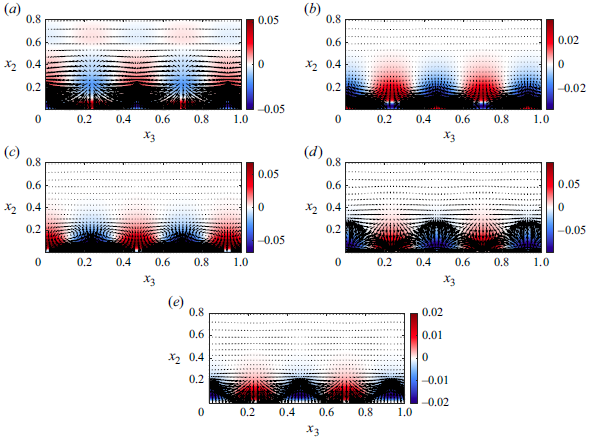
Responses of the first SPOD mode of the (a) streamwise, (b) wall-normal, (c) spanwise, (d) density-related and (e) the temperature-related forcing components in the cross-stream plane at
 $(\lambda _1^+,\lambda _3^+,c)=(465,96,0.63)$
, in the adiabatic turbulent boundary layer. Red and blue contours denote positive and negative streamwise velocity (
 $u_1$
) disturbances. The arrows represent the wall-normal (
 $u_2$
) and spanwise (
 $u_3$
) velocity components of the vortices.

The corresponding responses of the first SPOD mode of the five forcing components are then calculated through the linear resolvent operator, and their shapes in the cross-stream (
 $x_3$
–
 $x_2$
) plane are plotted in figure 10, at
 $(\lambda _1^+,\lambda _3^+,c)=(465,96,0.63)$
in the adiabatic turbulent boundary layer. In figure 10(a) the response of streamwise velocity (denoted by the red and blue contours) driven by the streamwise forcing (
 $\hat {f}_{1,e,\textit{SPOD}1}$
) is mostly clustered within a near-wall region (say,
 $x_2\lt 0.05$
in the present case), with the positive perturbations (red) accompanied with downward motions and the negative perturbations (blue) with upward motions. This is essentially consistent with the characteristics of sweep and ejection structures. In the region where the lift-up effect is active (Abreu et al. Reference Abreu, Cavalieri, Schlatter, Vinuesa and Henningson2020),
 $\hat {f}_{2,e,\textit{SPOD}1}$
and
 $\hat {f}_{3,e,\textit{SPOD}1}$
induce the occurrence of streamwise vortices. The vortical motions are observed between low-speed and high-speed streaks in figure 10(b,c), leading to the formation and amplification of streaks of streamwise velocity (Hamilton, Kim & Waleffe Reference Hamilton, Kim and Waleffe1995). On the other hand, the signs of streamwise velocity perturbations in response to
 $\hat {f}_{2,e,\textit{SPOD}1}$
and
 $\hat {f}_{3,e,\textit{SPOD}1}$
are opposite to each other in most regions, which suggests that in regions where the wall-normal forcing pushes the flow in the positive direction, the spanwise forcing yields negative fluctuations. The phenomenon of destructive interference is also observed between
 $\hat {f}_{1,e,\textit{SPOD}1}$
and
 $\hat {f}_{2,e,\textit{SPOD}1}$
and between
 $\hat {f}_{1,e,\textit{SPOD}1}$
and
 $\hat {f}_{3,e,\textit{SPOD}1}$
in certain parts of the boundary layer that modulates the shapes and amplitudes of the coherent structures, which is also seen in minimal turbulent Couette flow (Nogueira et al. Reference Nogueira, Morra, Martini, Cavalieri and Henningson2021). In figure 10(d,e), similar flow responses to density-related and temperature-related forcing, for instance, sweeps and ejections, are observed. An exception occurs in the magnitude of the streamwise velocity fluctuations driven by
 $\hat {f}_{5,e,\textit{SPOD}1}$
, which is much smaller than those by
 $\hat {f}_{i,e,\textit{SPOD}1}$
(
 $i=1,2,3,4$
). It indicates that the streamwise response is relatively insensitive to the nonlinear component in the temperature equation.
For the large scale
 $(\lambda _1,\lambda _3,c)=(2.85,1.06,0.75)$
in the adiabatic turbulent boundary layer, the response shapes of the first SPOD mode of the forcing terms are given in figure 11. It is evident that the structures become larger in both width and height than those at a smaller scale, in line with expectations. Findings in figure 11 are generally similar to those discussed for the small scale, in terms of the flow responses (sensitivity) to various forcing components. However, the magnitude of the streamwise velocity response of
 $\hat {f}_{1,e,\textit{SPOD}1}$
, as shown in figure 11(a), is comparable to that of
 $\hat {f}_{5,e,\textit{SPOD}1}$
, and it is nearly one order of magnitude smaller than the response to the other forcing components. It hence suggests that the influence of the streamwise forcing on the flow field is attenuated at this specific scale and specific location in the adiabatic case. Nevertheless, this trend is not discovered in the cold-wall case, as presented in Appendix B. Vortical motions appear as a result of the wall-normal and spanwise forcing, which have opposite impacts on the generation of velocity perturbations. This is consistent with the observations in the incompressible channel flows (Morra et al. Reference Morra, Nogueira, Cavalieri and Henningson2021). At last, the roles of
 $\hat {f}_{4,e,\textit{SPOD}1}$
and
 $\hat {f}_{5,e,\textit{SPOD}1}$
are mostly similar to each other, leading to velocity dilatation, although the magnitudes of the
 $u_1$
response induced by
 $\hat {f}_{5,e,\textit{SPOD}1}$
is much less pronounced than those by
 $\hat {f}_{4,e,\textit{SPOD}1}$
. In figure 11(d,e), positive and negative
 $u_1$
perturbations alternate along the spanwise direction, with the positive streamwise perturbations associated with vertical motions towards the wall and the negative ones carried away from the wall. Beyond that,
 $\hat {f}_{4,e,\textit{SPOD}1}$
and
 $\hat {f}_{5,e,\textit{SPOD}1}$
are found to result in opposite motions in the spanwise direction in most of the regions (say,
 $x_2\gtrsim 0.1$
).
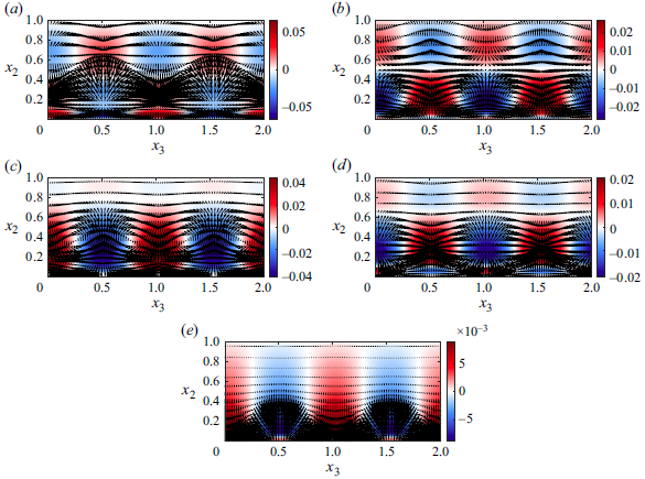
For the cold-wall turbulent boundary layer, the phenomena in velocity responses to each component of the reduced-order forcing are basically in alignment with the findings in the adiabatic case, indicating that the wall temperature will not essentially alter the dynamical physics at the current flow speed. It hence allows us to model the flow field in a general paradigm, in varying wall-temperature scenarios. The detailed discussion for the cold-wall case is not provided here for brevity, but is shown in Appendix B.
Responses of the first SPOD mode of the (a) streamwise, (b) wall-normal, (c) spanwise, (d) density-related and (e)the temperature-related forcing components in the cross-stream plane at
 $(\lambda _1,\lambda _3,c)=(2.85,1.06,0.75)$
, in the adiabatic turbulent boundary layer.

4.2.2. Contribution of decomposed forcing components
In the linearised resolvent framework, the CSD of response and forcing are related by (4.5), which allows us to separately quantify the contribution of the correlation of every two forcing components to turbulent fluctuations. To this end,
 ${\boldsymbol{S}}_{{\!\boldsymbol{f}_{\!e}{\kern-1.5pt}\boldsymbol{f}_{\!e}}}$
is decomposed into 25 sub-blocks constituted of pairs of every two forcing components, i.e.
 ${\boldsymbol{S}}_{{\!\boldsymbol{f}_{\!e}{\kern-1.5pt}\boldsymbol{f}_{\!e}}}=\sum _{j=1}^5\sum _{i=1}^5{\boldsymbol{S}}_{{\!\boldsymbol{f}_{i,e}\boldsymbol{f}_{j,e}}}$
. Here
 ${\boldsymbol{S}}_{{\!\boldsymbol{f}_{i,e}\boldsymbol{f}_{j,e}}}$
is a zero matrix except at the location of the
 $ij$
th block, which is associated with the correlation of the
 $i$
th and
 $j$
th forcing part. As the matrix of the CSD is Hermitian, the energy response
 ${\boldsymbol{S}}_{{\boldsymbol{qq}}}$
is categorised into five terms in association with auto-correlations
 \begin{equation} {\boldsymbol{S}}_{{\boldsymbol{qq}}}^{ii}=\boldsymbol{H}_{\!e} {\boldsymbol{S}}_{{\!\boldsymbol{f}_{i,e}\boldsymbol{f}_{i,e}}} \boldsymbol{H}_{\!e}^\dagger , \quad\mathrm{with}\,\,i=1,2,3,4,5, \end{equation}
and ten terms with cross-correlations
 \begin{equation} {\boldsymbol{S}}_{{\boldsymbol{qq}}}^{ij}=\boldsymbol{H}_{\!e}\big({\boldsymbol{S}}_{{\!\boldsymbol{f}_{i,e}\boldsymbol{f}_{j,e}}}+{\boldsymbol{S}}_{{\!\boldsymbol{f}_{j,e}\boldsymbol{f}_{i,e}}}\big)\boldsymbol{H}_{\!e}^\dagger , \quad\mathrm{with}\,\,i,j=1,2,3,4,5 \,\,\mathrm{and}\,\,i\ne j. \end{equation}
Streamwise energy in response to various correlation components in the eddy-viscosity-corrected forcing CSD, at
 $(\lambda _1^+,\lambda _3^+)=(465,96)$
, in the adiabatic turbulent boundary layer. The black solid line denotes the time-averaged energy spectral density of streamwise velocity fluctuation calculated through DNS data, at the corresponding length scale.

Streamwise energy in response to various correlation components in the eddy-viscosity-corrected forcing CSD, at
 $(\lambda _1,\lambda _3)=(2.85,1.06)$
, in the adiabatic turbulent boundary layer.

Figures 12 and 13 plot the time-averaged profiles of streamwise energy
 ${E}_{u_1 u_1}^{ij} = \textit{diag}(\bar {\boldsymbol{S}}_{u_1 u_1}^{ij})$
, where the operator
 $\textit{diag}$
means extracting the diagonal elements of matrix, in response to various components of the forcing CSD. The definition of the time average follows (4.3). Note that in the following discussion the statistics of the response are all plotted in terms of their time-averaged quantities, aiming to capture the dominant contributing features in the eddy-viscosity-corrected forcing term and, thus, yield insight for the modelling of forcing to estimate time-averaged turbulent quantities, unless otherwise specified. The results in response to the temperature-related forcing correlations are not presented due to their limited contribution in contrast to the others, which is consistent with the aforementioned findings in reduced-order analysis. In figure 12(a) the contribution of nonlinear forcing components contained in the momentum equations is quantified at the small scale. It is observed that the cross-correlation of forcing (
 $ {\boldsymbol{S}}_{{\!\boldsymbol{f}_{i,e}\boldsymbol{f}_{j,e}}}$
,
 $i,j=1,2,3$
and
 $i\ne j$
), as denoted by the dashed lines, contributes negatively to streamwise turbulent energy to counterbalance the high amplitudes resulting from the auto-correlations especially of the wall-normal and spanwise forcing. This aligns well with the results for near-wall structures in incompressible channels (Morra et al. Reference Morra, Nogueira, Cavalieri and Henningson2021). The
 $E_{u_1 u_1}$
components associated with the wall-normal and spanwise forcing, including
 $E_{u_1 u_1}^{22}$
,
 $E_{u_1 u_1}^{33}$
and
 $E_{u_1 u_1}^{23}$
, exhibit values remarkably larger than those associated with the other components. It implies that the wall-normal and spanwise forcing play a significant role in generating streamwise fluctuations, which is probably attributed to the lift-up effects. The obvious difference in the contributions from streamwise, wall-normal and spanwise forcing highlights their distinct importance in the magnitude of the response, and hence, different models should be considered for streamwise, wall-normal and spanwise forcing components, differing from previous studies (Gupta et al. Reference Gupta, Madhusudanan, Wan, Illingworth and Juniper2021; Chen et al. Reference Chen, Cheng, Gan and Fu2023).
The density-related forcing also exerts a significant impact on the output, as examined in figure 12(b). The
 $E_{u_1 u_1}^{44}$
is greater than the full
 $E_{u_1 u_1}$
obtained from DNS in the near-wall region, nonetheless the two curves share a similar peak location. A dramatical negative contribution is observed in terms contributed by the cross-correlations, except the constructive interference between wall-normal and density-related forcing components as illustrated by the positive distributions of
 $E_{u_1 u_1}^{24}$
. It hence indicates that the streamwise response to the wall-normal forcing aligns with that in response to the density-related forcing component, which is seen in most portions of the boundary layer in figures 10(b) and 10(d). Therefore, the cross-coherence among different forcing components, i.e. the off-diagonal terms in the forcing CSD, plays significant roles in the quantitative response of turbulent fluctuations. In this sense, the rationality of forcing decorrelation in space and components, which is commonly assumed in previous studies on modelling (Morra et al. Reference Morra, Semeraro, Henningson and Cossu2019; Chen et al. Reference Chen, Cheng, Gan and Fu2023; Holford et al. Reference Holford, Lee and Hwang2023), will be assessed in the following.
For the large energetic scale in the adiabatic turbulent boundary layer, the influence of various forcing components on the streamwise energy is shown in figure 13, with the temperature-related forcing not presented for conciseness. Similarly to the findings for the small scales, the auto-correlation of wall-normal and spanwise forcing yields a more prominent output than that of the streamwise one in the inner region, as demonstrated in figure 13(a). Negative distributions are also observed in
 $E_{u_1 u_1}^{12}$
and
 $E_{u_1 u_1}^{23}$
in response to the cross subitems. Differences occur in the role of the streamwise--spanwise forcing correlation, in that it yields a positive contribution, meaning that the streamwise and spanwise forcing push the flow in the same direction especially in the outer energy-containing region where there appears a second peak. This phenomenon contradicts the observations in the incompressible channel flows at a large scale with a given frequency (Morra et al. Reference Morra, Nogueira, Cavalieri and Henningson2021) where they used the original nonlinear term as input without considering eddy viscosity. In figure 13(b), a positive magnitude of
 $E_{u_1 u_1}^{44}$
associated with the auto-correlation of the density-related forcing is observed mainly in the inner region. The cross-correlations, including the
 $S_{f_{1,e} f_{4,e}}$
(
 $S_{f_{4,e} f_{1,e}}$
),
 $S_{f_{2,e} f_{4,e}}$
(
 $S_{f_{4,e} f_{2,e}}$
) and
 $S_{f_{3,e} f_{4,e}}$
(
 $S_{f_{4,e} f_{3,e}}$
), act to yield a negative contribution to the streamwise energy, except that a positive distribution of
 $E_{u_1 u_1}^{24}$
is seen beyond
 $x_2^+ \approx 10$
and it peaks at a wall-normal location further away from that of
 $E_{u_1 u_1}^{44}$
, which can possibly be ascribed to the wall-normal transport.
For the cold-wall turbulent boundary layer, contributions of the forcing components to the streamwise velocity fluctuations are also examined, through matrix decomposition. In general, the conclusions drawn in the adiabatic case also apply here, e.g. the high amplitude of the output in response to the wall-normal and spanwise forcing components and the negative contribution of most of the cross-correlation subitems in the full forcing CSD. Nevertheless, there exist some distinguishing features in the specific distributions of the streamwise-energy response. At the representative small scale
 $(\lambda _1^+,\lambda _3^+)=(929,208)$
,
 $E_{u_1 u_1}^{11}$
is observed to be larger than
 $E_{u_1 u_1}^{22}$
in figure 14(a). At a relatively larger scale, shown in figure 15(a), the substantial role of the CSD of streamwise forcing in the response (
 $E_{u_1 u_1}^{11}$
) is more evidently seen, as it contributes dominantly to the inner energy peak. Rather than the positive
 $E_{u_1 u_1}^{13}$
discovered at the large scale in the adiabatic case (figure 13
a), the output from the streamwise-wall-normal forcing correlation (namely
 $E_{u_1 u_1}^{12}$
in figure 15
a) is now positive in the inner part of the boundary layer (
 $x_2^+\lt 30$
), indicating that the wall thermal condition is able to coordinate the phase coherence among the forcing components. On the other hand, in figures 14(b) and 15(b), the positive contribution of the cross-correlation of the wall-normal and density-related forcing is not observed for both scales.
Streamwise energy in response to various correlation components in the eddy-viscosity-corrected forcing CSD, at
 $(\lambda _1^+,\lambda _3^+)=(929,208)$
, in the cold-wall turbulent boundary layer.

Streamwise energy in response to various correlation components in the eddy-viscosity-corrected forcing CSD, at
 $(\lambda _1,\lambda _3)=(2.76,1.02)$
, in the cold-wall turbulent boundary layer.

4.2.3. Assumption of forcing decorrelation in space and components
In the resolvent-based estimation of turbulent statistics, accurate modelling of the input, i.e.
 ${\boldsymbol{S}}_{{\!\boldsymbol{f}_{\!e}{\kern-1.5pt}\boldsymbol{f}_{\!e}}}$
in (4.5), is a necessity. Given the fact that the full forcing CSD is a high-dimensional matrix varying with wavenumbers and frequency, it is a great challenge to fully recover the input with limited flow information known. Previous studies usually focused on the modelling of the diagonal components in the CSD matrix, with the forcing assumed to be decorrelated in space and components. In this section the influence of this assumption on the accuracy of turbulence estimation is interrogated by means of designating the input as a diagonal matrix
 $\boldsymbol{S}_{\boldsymbol{f}_{\!e}{\kern-1.5pt}\boldsymbol{f}_{\!e}}^\textit{diag}$
, i.e. retaining only the diagonal component in the full CSD matrix to be different from zero.
Energy spectral density of the streamwise velocity, wall-normal velocity, spanwise velocity, density and temperature in response to the diagonal components in the eddy-viscosity-corrected forcing CSD
 $\boldsymbol{S}_{\boldsymbol{f}_{\!e}{\kern-1.5pt}\boldsymbol{f}_{\!e}}^\textit{diag}$
, at (a–e)
 $(\lambda _1^+,\lambda _3^+)=(465,96)$
and (h–j)
 $(\lambda _1,\lambda _3)=(2.85,1.06)$
, in the adiabatic turbulent boundary layer. The wall-normal distribution of turbulent energy in each component obtained from DNS is also shown for comparison.

Figure 16 plots the wall-normal distribution of turbulent energy, including
 $E_{u_1 u_1}$
,
 $E_{u_2 u_2}$
,
 $E_{u_3 u_3}$
,
 $E_{\rho \rho }$
and
 $E_{TT}$
, as a result of
 $\boldsymbol{H}_{\!e} \boldsymbol{S}_{\!{\boldsymbol{f}_{\!e}{\kern-1.5pt}\boldsymbol{f}_{\!e}}}^\textit{diag} \boldsymbol{H}_{\!e}^\dagger$
, in the adiabatic turbulent boundary layer. For the small scale in panels (a–e), all the peak locations are well captured by the diagonal components in the forcing CSD, except that of the wall-normal energy, which illustrates that the assumption of decorrelated forcing is rational to some extent in that it is able to recover the basic characteristics in turbulent structures. However, the magnitudes are found to deviate from those calculated from DNS data when omitting the off-diagonal information in the forcing input. In panels (f–j) the output at the large scale is examined, with a similar phenomenon observed. The output of streamwise energy from the decorrelated forcing exhibits a near-wall peak at
 $x_2^+\approx 12$
, aligned with the lower-amplitude tip in the DNS result. On the other hand, beyond the near-wall peak, the estimated curve decreases gradually, losing part of the flow information in the outer region, in particular, in terms of the predominant energy peak where the characteristic large-scale motions reside. This could possibly be attributed to the neglected nonlinear wall-normal interactions. As for the wall-normal and spanwise energy, the peaks of the resolvent output share consistent locations with those in the DNS results, though exhibiting larger magnitudes. On the other hand, a surprisingly good agreement is observed in the recovery of density and temperature perturbations in
 $x_2^+\lt 300$
, in terms of both shapes and amplitudes of the profiles.
Energy spectral density of the streamwise velocity, wall-normal velocity, spanwise velocity, density and temperature in response to the diagonal components in the eddy-viscosity-corrected forcing CSD
 $\boldsymbol{S}_{\boldsymbol{f}_{\!e}{\kern-1.5pt}\boldsymbol{f}_{\!e}}^\textit{diag}$
, at (a–e)
 $(\lambda _1^+,\lambda _3^+)=(929,208)$
and (h–j)
 $(\lambda _1,\lambda _3)=(2.76,1.02)$
, in the cold-wall turbulent boundary layer.

For the cold-wall case, the responses of flow quantities to the diagonal components in the forcing CSD are quantified in figure 17. In general, the peak locations in the output of streamwise, wall-normal and spanwise velocity components can be approximately captured by
 $\boldsymbol{S}_{\!{\boldsymbol{f}_{\!e}{\kern-1.5pt}\boldsymbol{f}_{\!e}}}^\textit{diag}$
for both scales, as seen in figure 17(a–c, f–h). It confirms that this sparse input of a diagonal matrix is able to capture the dominant turbulence features, which are essentially associated with the good modelling performance of the eddy-viscosity-improved resolvent operator (Fan et al. Reference Fan, Kozul, Li and Sandberg2024b
). Hence, the assumption of decorrelated forcing can be exploited for an intuitive turbulence estimation. In particular, the output of
 $E_{\rho \rho }$
faithfully follows the profile of DNS results in the region
 $x_2^+\lt 300$
. However, for the temperature, the shape of the response differs from that of the DNS results, especially at the large scale
 $(\lambda _1,\lambda _3)=(2.76,1.02)$
. As shown in panel (j), the peak of the temperature response is located at approximately the same position (
 $x_2^+\approx 25$
) with that of the streamwise response in panel (f). However this does not conform to the real physics. In the presence of strong wall cooling, the temperature fluctuation will peak at a location further away from the wall than that of the streamwise velocity fluctuation, as obtained from the DNS results. It indicates that only considering the diagonal component of forcing may omit the major source of the underlying amplification mechanism for temperature, especially when the cross-correlation terms (e.g. the correlation between velocity and temperature) exhibit essentially different characteristics from those in the adiabatic case.
To further unravel the influence of the forcing input at various wall-normal distances on flow statistics, the diagonal matrix
 $\boldsymbol S_{{\boldsymbol{f}_{\!e}{\kern-1.5pt}\boldsymbol{f}_{\!e}}}^\textit{diag}$
is decomposed as
 \begin{equation} \boldsymbol{S}_{\!{\boldsymbol{f}_{\!e}{\kern-1.5pt}\boldsymbol{f}_{\!e}}}^\textit{diag}\!\left (x_2;\kappa _{1}, \kappa _{3}, \omega \right ) = \Sigma _{x_{2,\textit{ref}}=0}^{x_{2,\textit{ref}}=+\infty }\boldsymbol{S}_{\!{\boldsymbol{f}_{\!e}{\kern-1.5pt}\boldsymbol{f}_{\!e}}}^\textit{diag}\!\left (\kappa _{1}, \kappa _{3}, \omega , x_{2,\textit{ref}}\right )\!, \end{equation}
where
 $\boldsymbol{S}_{\!{\boldsymbol{f}_{\!e}{\kern-1.5pt}\boldsymbol{f}_{\!e}}}^\textit{diag} (\kappa _{1}, \kappa _{3}, \omega , x_{2,\textit{ref}} )$
denotes a matrix with only the forcing spectra at the location
 $x_{2,\textit{ref}}$
retained. In such way, the response CSD can be formulated as
 \begin{align} {\boldsymbol{S}}_{{\boldsymbol{qq}}}\!\left (x_2,x_2';\kappa _{1}, \kappa _{3}, \omega \right )&=\boldsymbol{H}_{\!e}\!\left (\kappa _{1}, \kappa _{3}, \omega \right )\!\left [\Sigma _{x_{2,\textit{ref}}=0}^{x_{2,\textit{ref}}=+\infty }\boldsymbol{S}_{\!{\boldsymbol{f}_{\!e}{\kern-1.5pt}\boldsymbol{f}_{\!e}}}^\textit{diag}\!\left (\kappa _{1}, \kappa _{3}, \omega , x_{2,\textit{ref}}\right ) \right ]\nonumber\\&\quad\times \boldsymbol{H}_{\!e}^\dagger \!\left (\kappa _{1}, \kappa _{3}, \omega \right ). \end{align}
Correspondingly, the
 ${\boldsymbol{S}}_{\boldsymbol{qq}}$
component dependent on the forcing statistics at
 $x_{2,\textit{ref}}$
is given by
 \begin{equation} {\boldsymbol{S}}_{{\boldsymbol{qq}}}\!\left (x_2,x_2';\kappa _{1}, \kappa _{3}, \omega , x_{2,\textit{ref}}\right )=\boldsymbol{H}_{\!e}\!\left (\kappa _{1}, \kappa _{3}, \omega \right )\boldsymbol{S}_{\!{\boldsymbol{f}_{\!e}{\kern-1.5pt}\boldsymbol{f}_{\!e}}}^\textit{diag}\!\left (\kappa _{1}, \kappa _{3}, \omega , x_{2,\textit{ref}}\right ) \boldsymbol{H}_{\!e}^\dagger \!\left (\kappa _{1}, \kappa _{3}, \omega \right ). \end{equation}
Using Parseval’s theorem (4.3), the output of time-averaged streamwise energy, i.e.
 $\textit{diag}(\bar {\boldsymbol{S}}_{\boldsymbol{u_1 u_1}} (x_2,x_2'; \kappa _{1}, \kappa _{3}, x_{2,\textit{ref}} ))$
, is quantified as a function of
 $x_{2,\textit{ref}}^+$
at each wall-normal distance in figure 18, at two representative space scales in the adiabatic turbulent boundary layer. In this sense, the total turbulent energy in response to the decorrelated forcing is obtained upon summing the quantity along the horizontal direction in the pseudocolour plot of figure 18 at every
 $x_2^+$
. For both scales, the streamwise response at
 $x_2^+$
is observed to be preferentially more intercorrelated with the input forcing at
 $x_{2,\textit{ref}}^+\gt x_2^+$
, suggesting that the local forcing acts to generate ‘inner-layer’ responses. This may account for the phenomenon that the resolvent-based model gives an unsatisfactory estimation of energy spectra at the wall-normal locations that are higher than the location of the input data (Towne et al. Reference Towne, Lozano-Duran and Yang2020). A similar phenomenon is also found in our following work on estimation.
Streamwise energy in response to the eddy-viscosity-corrected forcing at a specific wall-normal position
 $x_{2,\textit{ref}}^+$
, at (a)
 $(\lambda _1^+,\lambda _3^+)=(465,96)$
and (b)
 $(\lambda _1,\lambda _3)=(2.85,1.06)$
, in the adiabatic turbulent boundary layer. The dashed line denotes
 $x_{2,\textit{ref}}^+=x_2^+$
.

The same finding can be observed in the cold-wall case. As shown in figure 19, the response of streamwise velocity is closely related to the forcing spectra at a higher wall-normal position. On the other hand, the forcing input at
 $x_{2,\textit{ref}}^+$
leads to a fairly pronounced response at
 $x_{2}^+=x_{2,\textit{ref}}^+$
throughout the boundary layer, indicating that the resolvent response to forcing is strongly localised. This phenomenon is also seen in the adiabatic case in figure 18, though less evident than that shown herein. Hence, the magnitude of forcing input is essentially significant for turbulence estimation, highlighting the necessity of an appropriate modelling of the input dependent on the wall-normal distance (Gupta et al. Reference Gupta, Madhusudanan, Wan, Illingworth and Juniper2021), which will be taken into account in the estimation of turbulent fluctuations in § 4.3.
4.3. Modelling of forcing statistics
In a statistically steady dynamical system, the response CSD is found to be the solution of an algebraic Lyapunov equation with an arbitrary forcing (Farrell & Ioannou Reference Farrell and Ioannou1993). Hence, aiming to estimate the statistical spectral densities of flow perturbations, here we construct an algebraic Lyapunov equation for compressible turbulent boundary layers. To start with, the linearised governing equation is given by
 \begin{equation} \frac {\partial \tilde {\hat {\boldsymbol{q}}}}{\partial t} + \boldsymbol{L}_{\!e} \tilde {\hat {\boldsymbol{q}}} = \tilde {\,\hat {\boldsymbol{\!f}}}_{\!e}. \end{equation}
Note that this equation is different from (4.4), as in (4.13) we did not perform a Fourier transform in time. The superscript
 $\tilde {\hat {\cdot }}$
denotes the variables that are Fourier transformed in the streamwise and spanwise directions, i.e.
 \begin{equation} \tilde {\hat {\boldsymbol{q}}}\!\left (x_{2},t ; \kappa _{1}, \kappa _{3} \right ) =\iint _{-\infty }^{\infty } \boldsymbol{q}\!\left (x_{1}, x_{2}, x_{3}, t\right ) \mathrm{e}^{-\mathrm{i}\!\left (\kappa _{1} x_{1}+\kappa _{3} x_{3}\right )} \mathrm{d} x_{1} \mathrm{d} x_{3}. \end{equation}
With the forcing assumed to be white in time, i.e. the temporal correlation satisfies
 ${\boldsymbol{S}}_{\boldsymbol{f}_{\!e} \boldsymbol{f}_{\!e}}(t,t') = {\boldsymbol{S}}_{\boldsymbol{f}_{\!e} \boldsymbol{f}_{\!e}}\delta _d(t-t')$
, where
 $\delta _d$
is the Dirac function, the statistically steady-state response CSD is determined through a related Lyapunov equation,
 \begin{equation} \boldsymbol{L}_{\!e} \bar {\boldsymbol{S}}_{\boldsymbol{q}\boldsymbol{q}} + \bar {\boldsymbol{S}}_{\boldsymbol{q}\boldsymbol{q}}\boldsymbol{L}_{\!e}^\dagger -{\boldsymbol{S}}_{\boldsymbol{f}_{\!e} \boldsymbol{f}_{\!e}} = 0. \end{equation}
This equation can be directly solved with a Matlab function upon the modelling of the forcing CSD (
 ${\boldsymbol{S}}_{\boldsymbol{f}_{\!e} \boldsymbol{f}_{\!e}}$
). In the following, attention will be only paid to the modelling of the diagonal components in the forcing CSD, due to their capability in capturing the dominant characteristics of turbulent structures based on the previous discussion.
Streamwise energy in response to the eddy-viscosity-corrected forcing at a specific wall-normal position
 $x_{2,\textit{ref}}^+$
, at (a)
 $(\lambda _1^+,\lambda _3^+)=(929,208)$
and (b)
 $(\lambda _1,\lambda _3)=(2.76,1.02)$
, in the cold-wall turbulent boundary layer.

In this paper, two major factors are considered in the modelling of
 ${\boldsymbol{S}}_{\boldsymbol{f}_{\!e} \boldsymbol{f}_{\!e}}$
, in contrast to designating it as an identity operator. The first aspect is regarding the definition of the streamwise-forcing function dependent on the wall-normal distances. As seen in figure 7, the CSD maps of the eddy-viscosity-corrected streamwise forcing concentrate compactly around the diagonal line and exhibit peaks varying with wavelengths. Generally, it is hard to restore the quantitative profile of streamwise forcing in the wall-normal coordinate with only the mean flow field known. Nevertheless, it can be designed as a function of wall-normal distance to highlight some essential features inherent in the distribution of streamwise forcing. Firstly, the peak of the function locates at
 $x_{2,peak}^+=10$
for the adiabatic case and
 $x_{2,peak}^+=30$
for the cold-wall case, which yields a common
 $x_{2,peak}^\star \approx 20$
for both cases. The superscript
 $\star$
denotes normalisation by semi-local units (Huang, Coleman & Bradshaw Reference Huang, Coleman and Bradshaw1995). Secondly, the values of the streamwise forcing at the wall surface and beyond the boundary-layer height
 $\delta _{99}$
are 0. In this sense, a linearly distributed hat function is given to qualitatively describe the distribution of streamwise forcing, as
 \begin{equation} |\hat {f}_{1,e}| = \left \{ \begin{aligned} &\frac {1}{x_{2,peak}^+} x_2^+ \quad &\textrm {for}\quad & x_2^+ \leqslant x_{2,peak}^+, \\ -&\frac {1}{\delta _{99}^+ - x_{2,peak}^+} \big( x_2^+ - x_{2,peak}^+\big) +1 \quad &\textrm {for}\quad & x_{2,peak}^+ \lt x_2^+ \lt \delta _{99}^+, \\ & 0 \quad &\textrm {for}\quad & x_2^+ \geqslant \delta _{99}^+. \end{aligned} \right . \end{equation}
Note that, herein we have not specified the precise magnitude of forcing, but simply take the peak to be unity and independent of wavelengths, due to the lack of appropriate flow information. To enable the quantitative estimation of turbulence at all scales, auxiliary information in terms of energy spectra is needed, which will be introduced in the following.
The second aspect to consider is the amplitude ratio between different forcing components due to the distinct roles of velocity-, density- and temperature-related forcing in generating vortical structures (see figures 10 and 11). Inspired from the basic mathematical formulations of
 $\boldsymbol{f}_{\!e}$
in Appendix A where similar forms are found for each component, the ratios of the other forcing components (
 $\hat {f}_{i,e}, i=2{-}5$
) to the streamwise forcing (
 $\hat {f}_{1,e}$
) are determined through the ratio of root-mean-square values of wall-normal velocity, spanwise velocity, density and temperature perturbations to that of streamwise velocity perturbations. In this sense, we define the ratios based on the empirical laws of turbulent fluctuations (Pope Reference Pope2000; Zhang et al. Reference Zhang, Bi, Hussain and She2014) as
 \begin{equation} \frac {|\hat {f}_{2,e}|^2}{|\hat {f}_{1,e}|^2} =0.2, \quad\frac {|\hat {f}_{3,e}|^2}{|\hat {f}_{1,e}|^2} =0.2, \quad\frac {|\hat {f}_{4,e}|^2}{|\hat {f}_{1,e}|^2} = \left (\frac {1}{Pr_t} \frac {\textrm {d} \bar {\rho }}{ \textrm {d} \bar {u}_1}\right )^2, \quad\frac {|\hat {f}_{5,e}|^2}{|\hat {f}_{1,e}|^2} = \left ( \frac {1}{Pr_t} \frac {\textrm {d} \bar {T}}{\textrm {d} \bar {u}_1}\right )^2. \end{equation}
Consequently, the forcing CSD is given as a diagonal matrix with its diagonal components being
 \begin{equation} \textit{diag} \!\left ( {\boldsymbol{S}}_{\boldsymbol{f}_{\!e} \boldsymbol{f}_{\!e}} \right ) = \big[ |\hat {f}_{1,e}|^2, |\hat {f}_{2,e}|^2, |\hat {f}_{3,e}|^2, |\hat {f}_{4,e}|^2, |\hat {f}_{5,e}|^2 \big] . \end{equation}
Then the response CSD can be calculated via (4.15). The turbulent energy is hence obtained as
 $\boldsymbol{E}_{\boldsymbol{q} \boldsymbol{q}} (x_{2}; \kappa _{1}, \kappa _{3} ) = \textit{diag}(\bar {\boldsymbol{S}}_{\boldsymbol{q} \boldsymbol{q}} (x_{2}, x_{2}'; \kappa _{1}, \kappa _{3} ) )$
. As the forcing CSD in (4.16) does not give the exact magnitude of its distribution, this
 $\boldsymbol{E}_{\boldsymbol{q} \boldsymbol{q}}$
cannot provide the specific magnitude of turbulent energy but only manifest its wall-normal shape of distribution at each specific scale. Hence, additional flow data are introduced into the framework for a full-scale turbulence estimation. We measure and utilise the energy spectral density
 ${E}_{{q} {q}}^{\textit{meas}}$
in one specific wall-normal plane
 $x_{2}^{\textit{meas}}$
to adjust the estimation results, yielding the turbulent energy spectra
 ${E}_{{q} {q}}^{\textit{est}}$
at the estimation location
 $x_{2}^{\textit{est}}$
as
 \begin{equation} {E}_{{q} {q}}^{\textit{est}} \!\left (x_{2}^{\textit{est}}; \kappa _{1}, \kappa _{3}\right ) = \frac {{E}_{{q} {q}} \!\left (x_{2}^{\textit{est}}; \kappa _{1}, \kappa _{3}\right )}{{E}_{{q} {q}} \!\left (x_{2}^{\textit{meas}}; \kappa _{1}, \kappa _{3}\right )} {E}_{{q} {q}}^{\textit{meas}} \!\left (x_{2}^{\textit{meas}}; \kappa _{1}, \kappa _{3}\right ). \end{equation}
Estimation of (a–c) the two-dimensional pre-multiplied spectra of streamwise velocity and (d–f) the spanwise pre-multiplied spectra of streamwise velocity, at various wall-normal locations in the adiabatic turbulent boundary layer. In panels (a–c) the contour lines indicate 0.1, 0.3, 0.5, 0.7 and 0.9 of their maxima, from outside to inside. In panels (d–f), spectra are normalised by the maximum of the DNS curve so that the peak value of the DNS spectra is unity, i.e.
 $C=1/{\rm max}(\kappa _3 E_{u_1u_1}^{\textit{dns}})$
. The curves denoted by Est. (classical) are obtained by setting the
 ${\boldsymbol{S}}_{\!\boldsymbol{f}_{\!e} \boldsymbol{f}_{\!e}}$
as an identity matrix.

Figure 20 presents the estimated two-dimensional and one-dimensional pre-multiplied spectra of streamwise velocity at various wall-normal locations in the adiabatic turbulent boundary layer, in contrast to the corresponding DNS results. Two methods for the modelling of forcing are used and compared with each other, i.e. the present forcing model (4.16)–(4.18) and the classical one with
 ${\boldsymbol{S}}_{\boldsymbol{f}_{\!e} \boldsymbol{f}_{\!e}}=\boldsymbol{I}$
. The measurement plane is selected in the logarithmic region, i.e. at
 $x_{2}^{\textit{meas}}\approx 0.12$
(namely
 $x_{2}^{meas,+}\approx 50$
). In panel (a) the estimation results at a near-wall position
 $x_{2}^{est,+}= 10$
are found to deviate from its counterpart obtained from DNS, though both of them can roughly recover the shape of the two-dimensional spectra. The estimated pre-multiplied
 $E_{u_1 u_1}^{\textit{est}}$
peaks at a larger spanwise scale than the pre-multiplied
 $E_{u_1 u_1}^{\textit{dns}}$
calculated from DNS data, with the peak location of
 $\kappa _1 \kappa _3 E_{u_1 u_1}^{\textit{est}}$
at
 $(\lambda _1^+,\lambda _3^+)=(322,100)$
using the present model and at
 $(\lambda _1^+,\lambda _3^+)=(516,90)$
using the classical method, whereasthe peak location of
 $\kappa _1 \kappa _3 E_{u_1 u_1}^{\textit{dns}}$
is at
 $(\lambda _1^+,\lambda _3^+)=(368,70)$
. As more clearly seen in the one-dimensional spanwise pre-multiplied spectra in panel (d), with the present model, the estimated curve is shifted towards the larger spanwise wavelength in comparison with the DNS result, leading to an underestimation in the streamwise turbulent energy for the spanwise wavelength smaller than 100, whereas an overestimation is seen beyond that. However, for the estimation results using the classical forcing model (
 ${\boldsymbol{S}}_{\boldsymbol{f}_{\!e} \boldsymbol{f}_{\!e}}=\boldsymbol{I}$
), they are significantly larger than the DNS results, indicating that ignoring the spatial variation of the forcing statistics would causean inaccurate ratio of the perturbations’ magnitude.
Estimation of (a–c) the two-dimensional pre-multiplied spectra of temperature and (d–f) the spanwise pre-multiplied spectra of temperature, at various wall-normal locations in the adiabatic turbulent boundary layer.

A similar situation occurs for the estimation of streamwise energy from the proposed forcing model (4.16)–(4.18) at
 $x_{2}^{est,+}= 30$
in panels (b) and (e), with the spectral energy tending to concentrate at a slightly larger scale. It suggests that the scale dependence of the forcing model may be incorporated so as to calibrate the mismatch in scales. For example, the peak location of the forcing may be designated to vary with the spanwise wavelength, following the scaling law of the spanwise spectra of the streamwise velocity throughout the logarithmic region in semi-local units (Huang et al. Reference Huang, Duan and Choudhari2022). Relevant work is to be conducted in future work, and is not shown here as the main purpose of this section is to provide potential research directions for improvement in the resolvent-based turbulence estimation. Beyond the measurement plane, at
 $x_{2}^{est,+}= 100$
shown in panels (c) and (f), the distribution of
 $E_{u_1 u_1}^{\textit{est}}$
is skewed towards smaller scales in contrast to that of
 $E_{u_1 u_1}^{\textit{dns}}$
, indicating that the large-scale turbulent information is missed with an inner measurement plane. This is consistent with the finding in figures 18 and 19. Although the estimations of the one-dimensional spanwise pre-multiplied spectra of streamwise velocity using the original and the present method are close to each other (see panel f), the improvement in the two-dimensional spectra (see panel c) is obvious.
Similarly, the estimation of temperature fluctuations is also carried out, in light of their tremendous significance in high-speed turbulent flows. The results of the pre-multiplied spectra of temperature at
 $x_{2}^{est,+}=10$
,
 $30$
and
 $100$
from the measurement at
 $x_{2}^{meas,+}\approx 50$
are shown in figure 21. For
 $x_{2}^{est,+}=10$
in panel (a), the estimated spectra using the classical method are dramatically deviated from the real results. Whereas with the forcing model proposed, the estimation performance is improved and the map of the estimated spectra is slightly to the left of that obtained from DNS data, indicating that the spanwise wavelengths where the two peaks locate are consistent with each other as clearly presented by the one-dimensional spanwise pre-multiplied spectra in panel (d). Moreover, the estimated magnitudes of the temperature fluctuations are closer to the DNS results than those with
 ${\boldsymbol{S}}_{\boldsymbol{f}_{\!e} \boldsymbol{f}_{\!e}}=\boldsymbol{I}$
, which largely overestimate the temperature fluctuations. At the wall-normal location closer to the measurement plane, the performance of the estimation is improved moderately and the overestimation with the classical method still exists. At last, for the estimation plane at
 $x_{2}^{est,+}=100$
(panels c and f), the temperature fluctuation is overestimated at small scales using the present model, which is similar to the observation in the estimation of streamwise velocity fluctuations.
Estimation of the spanwise pre-multiplied spectra of (a) the streamwise velocity and (b) the temperature in the adiabatic turbulent boundary layer. The contour lines indicate 0.1, 0.3, 0.5, 0.7 and 0.9 of their maxima, moving from outside to inside.

Estimation of (a–c) the two-dimensional pre-multiplied spectra of streamwise velocity and (d–f) the spanwise pre-multiplied spectra of streamwise velocity, at various wall-normal locations in the cold-wall turbulent boundary layer.

Estimation of (a–c) the two-dimensional pre-multiplied spectra of temperature and (d–f) the spanwise pre-multiplied spectra of temperature, at various wall-normal locations in the cold-wall turbulent boundary layer.

Furthermore, figure 22 plots the estimated contours of the one-dimensional spanwise pre-multiplied spectra of streamwise velocity and temperature across the adiabatic turbulent boundary layer. Only the results at planes beneath the measurement plane are presented, which are of practical importance due to the high cost of both simulations and experiments to obtain the flow field especially in proximity to the wall. It is clearly seen that the forcing model proposed in the present study can greatly improve the estimation of turbulent statistics, especially in terms of the temperature fluctuations. As shown in figure 22, this method is able to approximately recover the shape of the energy spectra of both streamwise velocity and temperature, though deviations are still seen at large
 $\lambda _3^+$
and the wall-normal region very close to the wall (
 $x_2^+\lt 5$
). Hence, further research is required to optimise the modelling of the nonlinear forcing. For example, our preliminary trials have already shown that the displacement of the energy peak in the spanwise spectra can be alleviated when taking into account the scale dependence of the forcing model, which shows great promise in turbulence estimation.
Estimation of the spanwise pre-multiplied spectra of (a) the streamwise velocity and (b) the temperature in the cold-wall turbulent boundary layer.

In the cold-wall turbulent boundary layer, estimation results of the spectra of the streamwise velocity and temperature are shown in figures 23–25. In general, the present method improves the estimation in terms of both the two-dimensional and one-dimensional energy spectra with the measurement taken at
 $x_{2}^{meas,+}\approx 50$
, although both the methods overestimate the perturbations of the streamwise velocity and temperature at
 $x_{2}^{est,+}\approx 10$
and
 $30$
. A significant exception occurs in the two-dimensional pre-multiplied spectra of temperature in the near-wall region. As depicted in figure 24(a), two separate peaks are observed in the DNS results, which is associated with the increased coherence of thermal structures in both streamwise and spanwise directions, in the presence of strong wall cooling (Fan & Li Reference Fan and Li2023). This peculiar observation is missed in the current estimation, which consequently leads to an overestimation of the magnitude of temperature fluctuations especially in the region beneath
 $x_2^+\approx 18$
, where the mean temperature exhibits a maximum (figure 25
b).
5. Conclusion
This paper investigates the characteristics of the nonlinear forcing and its contribution to flow responses in the input–output framework of resolvent analysis, consequently yielding valuable information for the modelling of forcing statistics. Using the DNS databases of two compressible turbulent boundary layers under adiabatic- and cold-wall conditions, the nonlinear forcing term in the resolvent formulation is firstly quantified. Its PSD at two representative energetic scales is compared with that of the optimal forcing mode that is calculated from the right singular vector of the resolvent operator. Significant differences are observed between the two maps, where the PSD of the real nonlinear forcing is mostly concentrated in the near-wall region whereas that of the optimal forcing mode follows the critical-layer hypothesis as a result of the amplification mechanism of the resolvent operator. It hence highlights the necessity of quantifying and characterising the real nonlinear forcing terms. The role of eddy viscosity is also examined through comparing the CSDs of the streamwise forcing with and without the addition of eddy viscosity to resolvent operator. It is noted that the eddy-viscosity-corrected forcing tends to be spatially uncorrelated, indicating that spatial cross-coherence maybe neglected in the modelling of the eddy-viscosity-corrected forcing and hence making the modelling of the eddy-viscosity-corrected forcing potentially easier than that of the original one. Therefore, in this paper, investigations of the forcing influences on responses and the modelling of forcing are all based on the eddy-viscosity-corrected forcing terms.
Aiming to measure the importance of each forcing component in generating turbulent dynamics, the contributions of the eddy-viscosity-corrected forcing to flow responses are then examined, based on the resolvent-based linear input–output system. It is observed that the streamwise motions are almost insensitive to the temperature-related forcing. Wall-normal and spanwise forcing tends to push the streamwise motions in opposite directions. Furthermore, the streamwise response associated with the wall-normal and spanwise forcing components exhibits larger magnitudes than those associated with the other components, implying the distinct significance of the five forcing components in flow responses and hence suggesting that different models should be considered for streamwise, wall-normal and spanwise forcing components. Cross-coherence among different forcing components also yields substantial response of turbulent fluctuations to counterbalance the high amplitudes resulting from the auto-correlations. In this sense, the rationality of the assumption of forcing decorrelation in space and components (i.e. omission of the cross-coherence), which has been commonly adopted in turbulence estimation, is further appraised. Results have shown that the simplified forcing matrix is able to capture the dominant turbulence features, e.g the peak location of the turbulent energy, hence suggesting that this type of sparse input can be deployed for an intuitive estimation of turbulent statistics (at least in these canonical wall-bounded turbulent flows). Moreover, local forcing is able to cause inner-layer responses and generate prominent responses at the same location, which indicates that the distribution of the response outputs would be sensitive to the magnitude of the local forcing input. At last, different wall thermal conditions will not essentially change the forcing-response characteristics, hence allowing us to model the forcing statistics in a general paradigm in varying wall-temperature scenarios.
Finally, the statistical spectral densities of streamwise velocity and temperature fluctuations are estimated via an algebraic Lyapunov equation, given the model of the forcing CSD. Based on the current observations, attention is only paid to the modelling of the diagonal components in the CSD matrix. In contrast to simply setting it as an identity matrix, two aspects of modifications are considered, i.e. the wall-normal dependence of the streamwise forcing and the amplitude ratio among five forcing components, which are highlighted in the forcing-response discussion of DNS results. With this proposed forcing model, improved estimations of the streamwise velocity and temperature fluctuations are achieved in compressible turbulent boundary layers both with and without wall cooling, especially in terms of the magnitudes and the peak locations of the temperature spectra.
Funding
Funding support from the National Natural Science Foundation of China (under the Grant Nos. 123B2030 and 12372221) is acknowledged. The authors also acknowledge support from the joint Ph.D. framework (Program) of Shanghai Jiao Tong University and the University of Melbourne.
Declaration of interests
The authors report no conflict of interest.
Appendix A. Formulations for the nonlinear forcing term in compressible turbulent boundary layers
The non-dimensional compressible Navier–Stokes equations for a perfect heat-conducting gas are given as
 \begin{align}&\,\,\, \rho \!\left (\frac {\partial u_{i}}{\partial t}+u_{j} \frac {\partial u_{i}}{\partial x_{j}}\right )=-\frac {1}{\gamma M_\infty ^{2}} \frac {\partial p}{\partial x_{i}}+\frac {1}{{{Re}}} \frac {\partial }{\partial x_{j}}\!\left [\mu \!\left (\frac {\partial u_{i}}{\partial x_{j}}+\frac {\partial u_{j}}{\partial x_{i}}\right )+\lambda \frac {\partial u_{k}}{\partial x_{k}} \delta _{i j}\right ],\\[-6pt]\nonumber \end{align}
 \begin{align}&\qquad\qquad\qquad\qquad\qquad\qquad \frac {\partial \rho }{\partial t}+u_{j} \frac {\partial \rho }{\partial x_{j}}=-\rho \frac {\partial u_{j}}{\partial x_{j}},\\[-10pt]\nonumber \end{align}
 \begin{align}& \rho \!\left (\frac {\partial T}{\partial t}+u_{j} \frac {\partial T}{\partial x_{j}}\right )=-\,(\gamma -1) p \frac {\partial u_{i}}{\partial x_{i}}+\frac {\gamma }{{{Re}}} \frac {\partial }{\partial x_{j}}\!\left (k \frac {\partial T}{\partial x_{j}}\right ) \notag \\[5pt] &\qquad\qquad\qquad\qquad\,\, +\gamma (\gamma -1) \frac {M_\infty ^{2}}{{{Re}}} \!\left [\mu \frac {\partial u_{i}}{\partial x_{j}} \frac {\partial u_{i}}{\partial x_{j}}+\mu \frac {\partial u_{i}}{\partial x_{j}} \frac {\partial u_{j}}{\partial x_{i}}+\lambda \!\left (\frac {\partial u_{k}}{\partial x_{k}}\right )^{2}\right ]. \end{align}
The symbols are redefined herein to facilitate reading and understanding. Here
 $t$
is time,
 $x_k$
(
 $k$
= 1, 2, 3) represent the streamwise, wall-normal and spanwise directions,
 $u_k$
are the corresponding velocity components;
 $\rho$
,
 $p$
,
 $T$
are density, pressure and temperature;
 $\mu$
and
 $\lambda$
are the coefficients of the molecular and second viscosity, following the Stokes assumption
 $\lambda =-2/3\mu$
;
 $k$
is the heat conduction coefficient given by
 $\mu /Pr$
,
 $Pr$
is the molecular Prandtl number,
 $\gamma$
is the specific heat ratio and
 $\delta _{ij}$
is the Kronecker delta;
 $M_\infty$
denotes the free-stream Mach number and
 ${Re}$
is the Reynolds number defined by
 $\rho _\infty ^* u_\infty ^* \delta _{99}^* /\mu _\infty ^*$
, where
 $\delta _{99}$
is the
 $99\,\%$
boundary-layer thickness. The subscript
 $\infty$
denotes free-stream variables and the superscript
 $*$
denotes dimensional values. Otherwise, variables are non-dimensionalised by free-stream flow quantities. The system is closed with the ideal gas state equation
 $p=\rho T$
.
As all the high-order nonlinear contributions in the Navier–Stokes equations are represented within a single forcing term, its expression can be obtained from the equations for fluctuations of velocities, density and temperature. Without adding eddy viscosity to the resolvent operator, the nonlinear terms
 ${\boldsymbol{\tilde {f}}}= [{\tilde {f}}_1,{\tilde {f}}_2,{\tilde {f}}_3,{\tilde {f}}_4,{\tilde {f}}_5 ]^{\top }$
in the physical domain for compressible turbulent boundary layers are given as
 \begin{align}& \tilde {f}_{i(i=1,2,3)} = -\left ( \frac {\partial \rho u_i' u_{\!j}'}{\partial x_j} - \frac {\partial \overline {\rho u_i' u_{\!j}'}}{\partial x_j} \right ) -\frac {\partial \rho ' u_i'}{\partial t} - \bar {u}_j \frac {\partial \rho ' u_i'}{\partial x_j} - \rho 'u_{\!j}'\frac {\partial \bar {u}_i }{\partial x_j} + N(\tau ),\\[-10pt]\nonumber \end{align}
 \begin{align}&\qquad\qquad\qquad\qquad\qquad\qquad\qquad\quad \tilde {f}_{4} = -\frac {\partial \rho ' u_{\!j}'}{\partial x_j},\\[-10pt]\nonumber \end{align}
 \begin{align}&\qquad\qquad \tilde {f}_{5} = -\left ( \frac {\partial \rho u_{\!j}' T'}{\partial x_j} - \frac {\partial \overline {\rho u_{\!j}' T'}}{\partial x_j} \right )-\frac {\partial \rho ' T'}{\partial t} - \bar {u}_j \frac {\partial \rho ' T'}{\partial x_j} - \rho 'u_{\!j}'\frac {\partial \bar {T}}{\partial x_j} \notag \\[4pt]&\qquad\qquad\qquad + N(p_w)+ N(\tau _w)+ N(q), \end{align}
Responses of the first SPOD mode of the (a) streamwise, (b) wall-normal, (c) spanwise, (d) density-related and (e) the temperature-related forcing components in the cross-stream plane at
 $(\lambda _1^+,\lambda _3^+,c)=(929,208,0.66)$
, in the cold-wall turbulent boundary layer. Red and blue contours denote positive and negative streamwise velocity (
 $u_1$
) disturbances. The arrows represent the wall-normal (
 $u_2$
) and spanwise (
 $u_3$
) velocity components of the vortices.

Responses of the first SPOD mode of the (a) streamwise, (b) wall-normal, (c) spanwise, (d) density-related and (e) the temperature-related forcing components in the cross-stream plane at
 $(\lambda _1,\lambda _3,c)=(2.76,1.02,0.88)$
, in the cold-wall turbulent boundary layer.

where the single prime denotes the turbulent fluctuations with respect to the Reynolds average.
 $ N(\tau )$
gives the nonlinear process in the viscous stress in the momentum equation,
 $N(p_w)$
,
 $N(\tau _w)$
and
 $N(q)$
represent the nonlinear processes in the pressure work, viscous work and heat conduction in the energy equation. Their expressions are listed as follows:
 \begin{align}& N(\tau )=\frac {1}{{{Re}}} \frac {\partial }{\partial x_j}\!\left [\mu ^{\prime }\!\left (\frac {\partial u_i^{\prime }}{\partial x_j}+\frac {\partial u_j^{\prime }}{\partial x_i}\right )-\overline {\mu ^{\prime }\!\left (\frac {\partial u_i^{\prime }}{\partial x_j}+\frac {\partial u_j^{\prime }}{\partial x_i}\right )}+\lambda ^{\prime } \frac {\partial u_k^{\prime }}{\partial x_k} \delta _{i j}-\overline {\lambda ^{\prime } \frac {\partial u_k^{\prime }}{\partial x_k}} \delta _{i j}\right ],\\[-10pt]\nonumber \end{align}
 \begin{align}&\qquad\qquad\qquad\qquad N(p_w)=-(\gamma -1)\left (p^{\prime } \frac {\partial u_i^{\prime }}{\partial x_i}-\overline {p^{\prime } \frac {\partial u_i^{\prime }}{\partial x_i}}\right )\!,\\[-10pt]\nonumber \end{align}
 \begin{align}&\qquad\qquad\qquad\quad N(\tau _w)=\gamma (\gamma -1) \frac {M_{\infty }^2}{{{Re}}}\!\left [\tau _{i j}^{\prime } \frac {\partial u_i^{\prime }}{\partial x_j}-\overline {\tau _{i j}^{\prime } \frac {\partial u_i^{\prime }}{\partial x_j}}\;\right ],\\[-10pt]\nonumber \end{align}
 \begin{align}&\qquad\qquad\qquad\qquad N(q)=\frac {\gamma }{{Pr} {{Re}}} \frac {\partial }{\partial x_j}\!\left (\mu ^{\prime } \frac {\partial T^{\prime }}{\partial x_j}-\overline {\mu ^{\prime } \frac {\partial T^{\prime }}{\partial x_j}}\right ). \end{align}
Note that the superscript of a tilde is to distinguish the variable from
 $\boldsymbol{{f}}$
, which means the Fourier transform of
 $\boldsymbol{\tilde {f}}$
does not yield the
 $\,\hat {\boldsymbol{\!f}}$
in (2.3). Basically,
 $\,\hat {\boldsymbol{\!f}}$
is the Fourier transform of
 $\boldsymbol{f}= [f_{1}, f_{2}, f_{3}, f_{4}, f_{5} ]^{\top }$
, where
 \begin{align}& {{f}}_{i(i=1,2,3,5)}= {{\tilde {f}}_i}/{\bar {\rho }}, \end{align}
 \begin{align}&\qquad {{f}}_4={\tilde {f}}_4. \end{align}
As for the eddy-viscosity-corrected forcing
 ${\boldsymbol{\tilde {f}}}_{\!e}= [{\tilde {f}}_{1,e},{\tilde {f}}_{2,e},{\tilde {f}}_{3,e},{\tilde {f}}_{4,e},{\tilde {f}}_{5,e} ]^{\top }$
, they are obtained, with the oscillations of Reynolds stress and turbulent heat flux modelled, as
 \begin{align}&\qquad\quad \tilde {f}_{i,e(i=1,2,3)} = -\frac {\partial \rho ' u_i'}{\partial t} - \bar {u}_j \frac {\partial \rho ' u_i'}{\partial x_j} - \rho 'u_{\!j}'\frac {\partial \bar {u}_i }{\partial x_j} + N(\tau ),\\[-12pt]\nonumber \end{align}
 \begin{align}&\qquad\qquad\qquad\qquad\qquad\quad \tilde {f}_{4,e} = -\frac {\partial \rho ' u_{\!j}'}{\partial x_j},\\[-12pt]\nonumber \end{align}
 \begin{align}& \tilde {f}_{5,e} = -\frac {\partial \rho ' T'}{\partial t} - \bar {u}_j \frac {\partial \rho ' T'}{\partial x_j} - \rho 'u_{\!j}'\frac {\partial \bar {T}}{\partial x_j} + N(p_w)+ N(\tau _w)+ N(q). \end{align}
Similar relation holds for
 ${\boldsymbol{{f}}}_{\!e}$
and
 ${\boldsymbol{\tilde {f}}}_{\!e}$
, i.e.
 ${{f}}_{i,e}= {\tilde {f}}_{i,e}/\bar {\rho }$
(
 $i=1,2,3,5$
) and
 ${{f}}_{4,e}={\tilde {f}}_{4,e}$
.
Appendix B. Flow responses to reduced-order forcing in the cold-wall turbulent boundary layer
Figures 26 and 27 present the shapes of the velocity responses to the first SPOD mode of the forcing components in the cold-wall turbulent boundary layer. The characteristic wave speeds are selected at
 $c=0.66$
and
 $0.88$
for the small- and large-scale motions, respectively. Herein, the phenomena are well consistent with the findings in the adiabatic turbulent boundary layer. In most regions of the cross-stream plane, the positive responses of the streamwise velocity are carried towards the wall by either forcing component, whereas the negative streamwise responses are carried away from the wall. This is in alignment with the structures of sweeps and ejections. On the other hand, the wall-normal and spanwise forcing generate opposite streamwise fluctuations and induce the vortical structures between the high-speed and low-speed streamwise streaks. At last, the responses of velocities are relatively less sensitive to the temperature-related forcing, in contrast to the other forcing components, hence suggesting the priority of specific forcing components for estimating the velocities.