1. INTRODUCTION
Maritime containers were first introduced in the 1960s. Since then, liner shipping has been through high-speed development, almost independent of the world economy. At present, most shipping companies adopt a hub-and-spoke operating structure which consists of hub ports, feeder ports, main lines and feeder lines, to form a complex container shipping network system (Meng and Wang, Reference Meng and Wang2011a). The optimal design of a container shipping network with its huge investment has become an issue which arouses the increasing attention of shipping companies (Crainic, Reference Crainic2000). The costs in the shipping network with transhipment can be reduced due to the deployment of large ships giving economies of scale. Therefore, how to design the container shipping network and the deployment of the ships to minimise the total network cost is a major problem.
Most existing studies on the optimisation of container shipping networks are mainly focused on two aspects: tramp shipping and liner shipping networks. The problem of tramp shipping network design deals with ship routing or fleet deployment for transporting bulk cargo, and a transhipment operation is not necessary due to the large volume between each Origin-Destination (OD) pair (Meng and Wang, Reference Meng and Wang2011b; Moon et al., Reference Moon, Qiu and Wang2015). However, transhipment is popular in the liner shipping network to reduce the cost (Wang et al., Reference Wang, Meng and Sun2013). The problems of liner shipping network design have been extensively studied in the literature and it can be divided into three streams (see Ronen, Reference Ronen1983; Reference Ronen1993; Christiansen et al., Reference Christiansen, Fagerholt and Ronen2004; Reference Christiansen, Fagerholt, Nygreen and Ronen2007; Reference Christiansen, Fagerholt, Nygreen and Ronen2013; Meng et al., Reference Meng, Wang, Andersson and Thun2014; Tran and Haasis, Reference Tran and Haasis2015). The first stream concentrates on the design of a single liner ship route (e.g. Rana and Vickson, Reference Rana and Vickson1988; Reference Rana and Vickson1991; Shintani et al., Reference Shintani, Imai, Nishimura and Papadimitriou2007) or a few liner ship routes (e.g. Ting and Tzeng, Reference Ting and Tzeng2003; Meng and Wang, Reference Meng and Wang2011c). The second stream focuses on the design of liner hub-and-spoke shipping networks (e.g. Imai et al., Reference Imai, Shintani and Papadimitriou2009; Gelareh et al., Reference Gelareh, Nickel and Pisinger2010; Gelareh and Pisinger, Reference Gelareh and Pisinger2011; Meng and Wang, Reference Meng and Wang2011d; Meng et al., Reference Meng, Wang and Liu2012; Zheng et al., Reference Zheng, Meng and Sun2015) where containers can only be transhipped at hub ports. The third is the design of liner shipping networks where containers can be transhipped at any port. Container routing in such general networks is the most challenging. Most of the past work in this stream uses link-based multi-commodity flow formulations, or segment-based formulations or path-based formulations (Wang et al., Reference Wang, Meng and Sun2013). For example, Song et al. (Reference Song, Zhang and Guo2007) constructed a container shipping network of foreign trade in an economic zone considering freight volume, flow direction, ship type and transhipment. Wang et al. (Reference Wang, Meng and Sun2013) presented a mathematical model for generating container paths, helping liner shipping companies to manage the container flow in liner shipping networks with transhipment. This paper focuses on the design of liner shipping networks where containers can be transhipped at any port. However, for a large scale of nodes in a liner shipping network, with traditional solving algorithm, the optimisation model usually cannot efficiently achieve high quality results. For example, the traditional ant colony algorithm is effective only when the node scale of the container shipping network is less than 20 (Song et al., Reference Song, Zhang and Guo2007). In view of this, based on the directional property of container shipping routes, this paper introduces the concept of steering vector, to improve the ant colony algorithm proposed by Song et al. (Reference Song, Zhang and Guo2007) for efficiently solving the container shipping network optimisation problem. An optimisation model is proposed for minimising the total shipping cost of container flow. A Max-Min Ant System (MMAS) solving algorithm based on a steering vector search pattern is developed, and an orthogonal array method is adopted in parameter settings to obtain the container routing and deployment of container ships.
The remainder of this paper is organised as follows. Section 2 develops a container shipping network optimisation model. Section 3 illustrates the main characteristics of container shipping routes, together with an improved MMAS algorithm based on a steering vector search pattern. Numerical experiments are given in Section 4, followed by some conclusions, discussions and possible future extensions of this research in Section 5.
2. CONTAINER SHIPPING NETWORK OPTIMISATION MODEL
2.1. Problem description
Container shipping network G is a weighted graph, and it can be defined as G(N, A, W), where N is the port node set, the size of which is N
s; A represents the set of all the possible container routes between two port nodes. For any port node i, j (i, j ∈ N, i ≠ j), ij is the route from port i to port j; W is the weight set of container shipping routes, and the weight is the transport cost on the route ij per container. Define m as the ship type used on the shipping routes, d
ij
as the travelling distance from port i to port j, v
m
as the travelling speed of ship type m,
 $C_{ij}^{{\rm r},m} $
as the daily charter cost of ship type m on the route ij, and
 $q_{ij}^m $
as the traffic volume for ship type m on the route ij including the transhipment volume, then the weight on the route ij equals
 $\displaystyle{{C_{ij}^{{\rm r},m}} \over {q_{ij}^m}} \cdot \displaystyle{{d_{ij}} \over {24v_m}} $
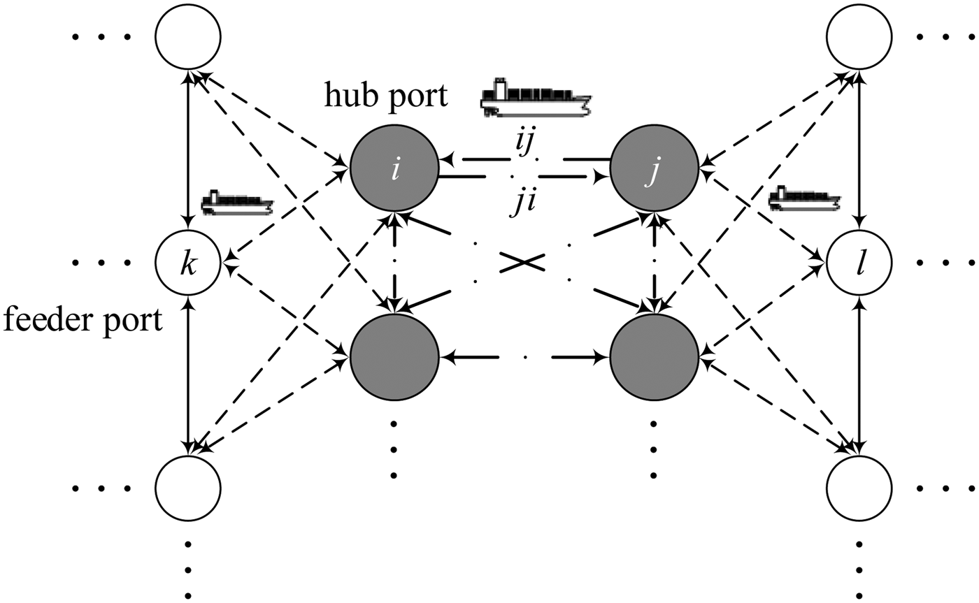
, and it changes with the ship type m deployed on the route which is determined by the traffic flow of OD pairs. Any container in the network can be considered as being carried by ship type m from departure port to destination port through transit ports. For example, as shown in Figure 1, containers are transported from departure port k to destination port l through two transit ports i and j where the container ship changes. Therefore how to choose the transit port and determine the ship type travelling on the shipping routes to minimise the total network cost is the key problem that needs to be solved in this paper. With two types of decision variables mentioned above, the optimisation model is nonlinear, and this problem is characterised as an NP-hard (Non-deterministic Polynomial-time hard) problem which is difficult to solve. The state space of feasible solutions grows exponentially with the increasing number of ports.
A sketch of container routing with transhipment.

Considering an Ns
-node network with no more than two transit ports during the tour, there are
 $\left( {{\rm C}_{N^S - 2}^1 \cdot {\rm C}_{N^S - 3}^1 + {\rm C}_{N^S - 2}^1 + 1} \right)^{N^S (N^S - 1)} $
combinations of solution space for the shipping routes. Taking a ten-node port network as an example, the number of traffic volumes for both flow directions of any two different ports in OD statistics is 90, and its scale of solution space reaches 6590. The scale of solution space is much larger when ship type m is considered. To overcome the large space and time complexity of the above problem, this paper constructs a container shipping network optimisation model and develops an effective solving algorithm combining MMAS solving algorithm with the steering vector search pattern.
2.2. Assumptions
Some assumptions are made regarding the shipping process to simplify the problem:
-
• The container shipping network is relatively stable, and emergency events are not considered in the model. We focus on the total yearly cost of the container shipping network, so it is reasonable to investigate the overall performance of the network over a long-term period without considering emergency events. Suppose that each ship route provides a weekly service frequency and consider a particular ship on each ship route. There are four weeks in a month and twelve months in a year. For stable network, a yearly service frequency equals the product of 48 and the weekly service frequency.
-
• The differences between loaded containers and empty containers are not considered. The design of container liner shipping networks considering empty container repositioning is a very sophisticated problem in the literature. For simplicity, we do not differentiate loaded and empty containers, and all traffic flow of OD pairs are converted into Twenty-foot Equivalent Units (TEUs). The loading capacity and traffic volume of various ship types are measured by TEUs in the modelling process.
-
• The container traffic flow volume of any OD pair can be obtained according to the forecast of the throughput of the port and the economy level of the hinterland. We assume traffic flow of OD pairs are given in the optimisation process.
-
• The container shipping network is composed of a quantity of main and branch lines, and maritime cabotage legislation is not considered. Cabotage legislation applies to ships in most countries that have a coastline so as to protect the domestic shipping industry from foreign competition. With cabotage legislation, the number of national-flagged ships operating in domestic waters will be increased compared to that of foreign ships. Cabotage legislation is not considered in the general shipping network where containers can be transhipped at any port and all ship types have no ownership property in the modelling process.
2.3. Mathematical model
The optimisation model is built with the purpose of minimising the total cost of container routing. Container shipping's comprehensive costs are made up of two components: operation and capital costs. In general, the capital cost refers to the cost of the ship itself in the shipping process that is related to time, while the operation cost refers to the cost generated after the ship's arrival which is related to the ship type and the amount of cargo, including the costs of port entry, loading and unloading and waiting in port (Shintani et al., Reference Shintani, Imai, Nishimura and Papadimitriou2007).
2.3.1. Analysis of a container's shipping costs
A: Ship related costs
The ship related costs of ship type m on the shipping route ij (
 $C_{ij}^{{\rm S},m} $
) can be represented as Equation (1).
 $$C_{ij}^{{\rm S},m} = C_{ij}^{{\rm R},m} + C_{ij}^{{\rm F},m} $$
where
 $C_{ij}^{{\rm R},m} $
and
 $C_{ij}^{{\rm F},m} $
are the charter cost and fuel cost of ship type m on the shipping route ij, respectively. C
ij
R,m
is the compound function of the travelling time and the charter cost of the ship for each day, which can be calculated as Equation (2).
 $$C_{ij}^{{\rm R},m} = C_{ij}^{{\rm r},m} \cdot \left\{ {\displaystyle{{d_{ij}} \over {24v_m}} + \displaystyle{{\left[ {\left( {t_i^{{\rm h},m} + t_j^{{\rm h},m}} \right) \cdot q_{ij}^m + t_i^{{\rm w},m} + t_j^{{\rm w},m}} \right]} \over {24}}} \right\} = \displaystyle{{C_{ij}^{{\rm r},m} \cdot \left[ {\left( {t_i^{{\rm h},m} + t_j^{{\rm h},m}} \right) \cdot q_{ij}^m} \right]} \over {24}} + C_{ij}^{{\rm r},m} \cdot \tau _{ij}^m $$
where
 $C_{ij}^{{\rm r},m} $
is the charter cost of ship type m per day on the shipping route ij, and it can be calculated by referring to the market report of container shipping;
 $t_i^{{\rm h},m} $
is the average handling time for a container at port i;
 $t_i^{{\rm w},m} $
is the average standby time for ship's arrival or departure at port i;
 $\tau _{ij}^m $
is represented as Equation (3).
 $$\tau _{ij}^m = \displaystyle{{\left[ {t_i^{{\rm w},m} + t_j^{{\rm w},m}} \right]} \over {24}} + \displaystyle{{d_{ij}} \over {24v_m}} $$
The fuel cost of ship type m includes the fuel consumption cost and the lubrication oil consumption cost, which is shown as Equation (4).
 $$C_{ij}^{{\rm F},m} = \displaystyle{{\left( {C_{ij}^{{\rm Fuel},m} R_{ij}^{{\rm Fuel},m} + C_{ij}^{{\rm Lub},m} R_{ij}^{{\rm Lub},m}} \right) \cdot HP_m \cdot d_{ij}} \over {v_m}} $$
where C ij Fuel,m and C ij Lub,m are the fuel and lubrication oil consumption cost per unit, respectively; R ij Fuel,m and R ij Lub,m are the fuel and lubrication oil consumption; HP m is the engine power of ship type.
B: Port related costs
The port related costs of ship type m on the shipping route ij (C ij P,m ) can be represented as Equation (5).
 $$C_{ij}^{{\rm P},m} = C_{ij}^{{\rm I},m} + C_{ij}^{{\rm H},m} $$
where
 $C_{ij}^{{\rm I},m} $
is the additional cost of port entry, including the shipping tonnage duty, berthing fee, pilotage fee, and the charge for tug services, etc.;
 $C_{ij}^{{\rm H},m} $
is the handling cost, which is in the linear function of
 $q_{ij}^m $
, that is,
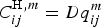 $C_{ij}^{{\rm H},m} = Dq_{ij}^m $
, D is the coefficient.
C: Total cost of the container shipping network
The total cost of a container ship of type m on the shipping route ij in the network
 $C_{ij}^{{\rm T},m} $
is expressed as Equation (6).
 $$C_{ij}^{{\rm T},m} = C_{ij}^{{\rm S},m} + C_{ij}^{{\rm P},m} $$
Therefore, the total yearly cost of the container shipping network is shown in Equation (7).
 $$C^{\rm T} = \sum\limits_{i = 1}^{N^{\rm S}} {\sum\limits_{\,j = 1,\ j \ne i}^{N^{\rm S}} {\sum\limits_{m = 1}^M {48 \cdot \rho _{ij}^m \cdot C_{ij}^{{\rm T},m}}}} $$
where M is the size of ship type set;
 $\rho _{ij}^m $
is the ship service frequency (ships/week), which is related to the container shipment volume and the ship type between two ports.
2.3.2. Model foundation
The objective function of the optimisation model minimises the total yearly cost of the container shipping network, which can be expressed as Equation (8).
 $$\mathop {\min }\limits_{\delta _{kl}^{ij} ,\varphi _{ij}^m } C^{\rm T} = \mathop {\min }\limits_{\delta _{kl}^{ij} ,\varphi _{ij}^m } \sum\limits_{i = 1}^{N^{\rm S}} {\sum\limits_{\,j = 1,\ j \ne i}^{N^{\rm S}} {\sum\limits_{m = 1}^M {48\varphi _{ij}^m \cdot \rho _{ij}^m \left\{ \matrix{\left\{ {\sum\limits_{k = 1}^{N^{\rm S}} {\sum\limits_{l = 1,l \ne k}^{N^{\rm S}} {C_{ij}^{{\rm r},m} \left( {\displaystyle{{t_i^{{\rm h},m} + t_j^{{\rm h},m} } \over {24}}} \right) + D} } } \right\} \cdot q_{kl}^m \cdot \delta _{kl}^{ij} \hfill \cr + C_{ij}^{{\rm F},m} + C_{ij}^{{\rm I},m} + C_{ij}^{{\rm r},m} \cdot \tau _{ij}^m \hfill} \right\}} } } $$
where
 $\varphi _{ij}^m $
is the decision variable which indicates whether ship type m is chosen for the shipping route ij; when m is selected,
 $\varphi _{ij}^m $
is 1; otherwise,
 $\varphi _{ij}^m $
is 0; kl is the shipping route between port k and port l;
 $\delta _{kl}^{ij} (i \ne j \ne k \ne l)$
is the binary decision variable, which indicates whether the traffic volume
 $q_{kl}^m $
is carried on the shipping route ij; when the containers carried from port k to port l are transported on the shipping route ij,
 $\delta _{kl}^{ij} $
is 1, otherwise;
 $\delta _{kl}^{ij} $
is 0.
Each
 $\delta _{kl}^{ij} $
corresponding with
 $q_{kl}^m $
is an Ns
× Ns
sparse matrix. The sum of all elements in the sparse matrix
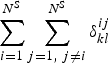 $\sum\limits_{i = 1}^{N^{\rm S}} {\sum\limits_{j = 1,\ j \ne i}^{N^{\rm S}} {\delta _{kl}^{ij}}} $
is the number of transit ports plus 1. In fact, most of the containers can be transferred at most twice in the real world container network. When
 $\delta _{kl}^{kl} = 1$
(i = k, j = l), all containers are transported from port k to port l directly without passing through other ports. How to determine the very few non-zero elements in the matrix efficiently is the key to solving this problem. Besides, some constraints are described as follows.
 $$1 \les \sum\limits_{i = 1}^{N^{\rm S}} {\sum\limits_{\,j = 1,\ j \ne i}^{N^{\rm S}} {\delta _{kl}^{ij}}} \les L + 1$$
 $$\sum\limits_{\,j = 1,\ j \ne i}^{N^{\rm S}} {q_{ij}} \les P_i $$
 $$\sum\limits_{\scriptstyle k = 1 \hfill \atop \scriptstyle k \ne j \hfill} ^{N^s} {\sum\limits_{\scriptstyle l = 1 \hfill \atop \scriptstyle l \ne k,l \ne j \hfill} ^{N^s} {\left( {\sum\limits_{\scriptstyle i = 1 \hfill \atop \scriptstyle i \ne j \hfill} ^{N^s} {q_{kl} \cdot \sigma _{kl}^{ij}} - \sum\limits_{\scriptstyle i = 1 \hfill \atop \scriptstyle i \ne j \hfill} ^{N^S} {q_{kl} \cdot \sigma _{kl}^{\,ji}}} \right)}} = 0$$
 $$i,j,k,l \in N,\;i \ne j,k \ne l$$
Constraint Equation (9) limits all containers to be transferred no more than twice during the tour when the number of transit ports L equals 2. Constraint Equation (10) indicates that the total container volume cannot exceed the throughput of the port. Constraint Equation (11) means that there must be an output for each input transit container.
3. SOLUTION PROCEDURE
3.1. Characteristics of container shipping route
Due to the high daily cost of a large ship, container shipping routes in the real world generally have the following characteristics:
-
• Although transporting containers from feeder port to hub port where a groupage occurs can reduce the transport cost to some extent, the transition of the ships also imposes additional costs, such as port charges. These additional costs will increase with the growth of transit nodes. Therefore the number of transit nodes cannot be large (usually does not exceed two), as shown in Figure 2. This characteristic of container shipping route is reflected in constraint Equation (9) of the optimisation model given in the previous section.
-
• No matter how a container transits, it always flows roughly towards the destination port. In the case of far-distance lines (the distance between transit port and departure port or destination port is long), the angle between transit route and direct route will not exceed 90°. While in the case of short-distance lines (for example, transit port and departure port or destination port are in the same region), it may be larger than 90°, as shown in Figure 2.
-
• Reverse-directional transport is less likely to appear in far-distance container shipping, as shown in Figure 3.
Characteristics of container shipping.

Unreasonable container shipping route.

3.2. Steering vector search pattern
Based on the characteristics of a container shipping route, we propose to utilise the concept of “steering vector search pattern” to improve the search mechanism in the solution algorithm by reducing the search range of the transit nodes. For convenience, a search pattern that does not adopt steering vector is labelled as “random search pattern”.
Suppose there are n port nodes in the network and the nodes closer to each other fall into a set of Y. All of the nodes are divided into a total of i sets, that is, Y i = {X i1, X i2, …, X ij | X ij is the j th node of set i}. For an arbitrary OD whose departure port and destination port are not in the same set, Y is sorted by the direction from departure port to destination port in accordance with the second and third characteristics of the container shipping route, and make up a new set SY = {Y 1, Y 2, …, Y k }, as shown in Figure 4. Set SY is defined as the steering vector set in the search process of the transit nodes. For the OD of reversed route, the elements of SY are arranged in opposite order, i.e., SY = {Y k , Yk −1, …, Y 1}. The algorithm searches the set Y i in turn following the direction pointed by the steering vector, and chooses or abandons transit ports in Y i according to a random search pattern. The problem of orientation will not exist if departure port and destination port are in the same set Y i , and in this case transit port can be chosen or abandoned following the random search pattern.
Steering vector search pattern.

Under a random search pattern, any route has no more than two transit nodes in the results of the optimisation model, so the search range of transit nodes is n-2 nodes. For a steering vector search pattern considering the characteristics of the container shipping route, the search range is reduced to the nodes contained in set SY, and the searching is conducted in the order of {Y 1, Y 2, … , Y k }. For any route, not only the number of nodes will be reduced by varying degrees, but also the searching will be in accordance with the established direction, so the search pattern can be simplified. The essence of the steering vector search pattern is converting the original large-scale random pattern into a combination of some smaller-scale and simpler random models, without changing the internal mechanism of the model. Therefore compared to the same scale random pattern, the introduction of steering vector can reduce the search range of transit nodes.
3.3. An improved MMAS algorithm based on steering vector search pattern
The applications of ant colony algorithms have spread widely, and the algorithm itself has been refined and improved to form a series of ant colony optimisation algorithms. This paper adopts the MMAS algorithm designed by Stützle and Hoos (Reference Stützle and Hoos2000) to limit the range of pheromone, and to avoid premature convergence due to large differences of pheromone during the run of the algorithm.
A bionic network system is advanced in this paper. Each port node is assumed to be “food” with different allure to ants, and shipping routes between ports are treated as the links connecting the food, so all the ports are put into a multi-node and multi-way connection chart. Initially, e ants are placed on randomly chosen nodes of the n ports, and ready to start. The probability of each link selected by the ant is determined by its pheromone intensity τ ij and value of the visibility η ij . ηij is set equal to l ij , where l ij means the density of container flow on link (i, j).
Owing to the steering vector, the ant with a sense of direction can perceive the destination, and does not go backwards or off course. It tends to choose the link with a lower cost which means the ant only selects the next node having a lower OD cost than the current one. An ant k currently located at node i chooses to go to node j with a probability (Dorigo, Reference Dorigo1992):
 $$P_{ij}^k (t) = \left\{ {\matrix{ {\displaystyle{{\tau _{ij}^\alpha (t) \times \eta _{ij}^\beta (t)} \over {\sum\limits_{u \in {\rm allowed}_k} {\tau _{iu}^\alpha (t) \times \eta _{iu}^\beta (t)}}}} & {\,j \in {\rm allowed}_k} \cr 0 & {{\rm otherwise}} \cr}} \right.$$
where α and β are two stimulating factors which determine the relative importance of the orbits and the visibility; allowed k is the set of nodes which can be selected by ant k in the next step.
In order to focus the search on the neighbourhood space of the optimal solution, the ant selects the next node s by introducing a pseudo-random proportional rule (Zhang et al., Reference Zhang, Sun and Tan2002) as below:
 $$s = \left\{ {\matrix{ {{\rm arg}\;\mathop {{\rm max}}\limits_{\,j \in {\rm allowed}_k} (\tau _{ij}^\alpha \times \eta _{ij}^\beta )} & {q \les q_0} \cr S & {{\rm otherwise}} \cr}} \right.$$
where q is a random number uniformly distributed between 0 and 1, q 0 is a given parameter (0 ⩽ q 0 ⩽ 1), and S are random variables selected according to the probability distribution given by Equation (13). When an ant located at the node i chooses the next node j, it selects a random number q. if q ⩽ q 0, the ant will choose the best link according to a priori knowledge, otherwise, select another link according to the probability calculated by Equation (13).
The principle of pheromone update is that only the global optimum ant is allowed to release pheromone to conduct the global update. After all of the ants have completed the tour, the program retrieves the elite ant with the lowest cost, saves its various kinds of information and has a global update to the pheromone density of the route. The pheromone updates (Toksari, Reference Toksari2006) as follows:
 $$\tau _{ij} (t + 1) = (1 - \rho ) \cdot \tau _{ij} (t) + \Delta \tau _{ij}^{{\rm opt}} $$
 $$\Delta \tau _{ij}^{{\rm opt}} = \displaystyle{E \over {\,f_{gb}}} $$
where ρ (with 0 < ρ < 1) is the volatile factor of pheromone, reflecting the strength of individual interactions among ants; E represents the intensity of pheromone which equals the total amount of pheromone after a search; f gb denotes the global optimal function value.
To avoid stagnation, τ ij is limited to an interval [τ min, τ max] in the algorithm. When we update the pheromone, if we have τ ij > τ max, we set τ ij = τ max; analogously, if τ ij < τ min, we set τ ij = τ min.
When the search of all the feasible OD routes is completed, a set including all of the candidate routes can be obtained, from which we can select the scheme with the lowest total network cost and record various information on the ants. Then a global update on the pheromone is conducted according to the elite-ant strategy, and the data of the container flow on the network route can be amended.
At this point, a search of the minimum total cost of the network is finished, and the optimal container shipping network is formed. If the model reaches termination condition, it will output the results, otherwise, replace the OD nodes in sequence, and go back and continue a new round of optimisation until it reaches the pre-set number of cycles.
3.4. Parameter settings of MMAS model algorithm
There is no rigorous theoretical basis for parameter settings of MMAS algorithms as yet (Duan, Reference Duan2005). In this paper, the parameters mainly include the number of ants e, information stimulating factor α, expected stimulating factor β, volatile factor of pheromone ρ and intensity of pheromone E. Based on a large number of numerical simulations and the characteristics of the algorithm itself, an orthogonal array method is applied to set the algorithm parameters.
The basic idea of orthogonal methods is the use of appropriate orthogonal arrays to optimise parameters, where the least-squares principle is usually adopted. That is to seek θ
i
(i = 1, …, r) to make
 $z = \sum\limits_{i = 1}^n {\left[ {y_i - f(x_1, \cdots, x_i, \theta _1, \cdots, \theta _r )} \right]^2} $
the smallest, where θ
1,…, θ
r
are undetermined parameters. (y
i
, x
1, … , x
i
) (i = 1, …, n) is n-group of measurements of the independent variables x
1, … , x
i
and the dependent variable y (Sun et al., Reference Sun, Song, Zhang, Liu and Wang2004).
The orthogonal array is normally credited to L a (cb ) and indicates that it can arrange up to a experiments with b factor and c level factors. The experiment program arranged by the orthogonal array is characteristic of balanced collocation and the factors between each other are orthogonal.
The process of making the initial orthogonal array can be described as follows:
-
• An appropriate orthogonal array is selected according to the number of parameters r.
-
• The middle value within the scope of known parameters is used as the middle bit level.
-
• The initial bit level factors u is set for each parameter.
-
• The middle bit level is denoted by θ i0 in position i 0, and the value of the bit level i is θ i = θ i0 u (i−i0)(i = 1, 2, …, i 0, …, 2i 0 − 1).
Accordingly, the optimum calculation schemes of the initial orthogonal parameters can be determined, and the method is as follows:
-
• Referring to the relevant references, a reasonable and larger range in accordance with the empirical value of the parameters of the similar problem is determined.
-
• With a lower number of cycles, the orthogonal method is adopted to do calculations on the initial collocation of parameters. Analysis on optimal results shows that the number of ants e is not affected by the collocation of parameters, while parameters (α, β, ρ, E) are greatly affected.
-
• The parameters (α, β, ρ, E) are fixed to get a better result, and the optimal value of e is determined by adjustment and trial.
-
• The algorithm obtains the combinations of the parameters (α, β, ρ, E) into the model according to the orthogonal array method and trials and adjusts repeatedly, then determines the optimal values of the collocation of the parameters.
4. NUMERICAL EXPERIMENTS
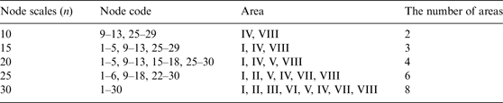
In this paper, a number of ports are selected from each region of the three major international routes (Europe-East Asia-North America) to form the container shipping network consisting of 30 ports, as shown in Figure 5. We need to predict the container throughput of each port in 2015 from a shipping company. However, the studies of prediction method are not the main contents of this paper. In order to simplify the calculation, only linear regression of time series methods is used to predict the OD distribution of containers. The horizontal comparisons among five types of networks, which have different numbers of nodes, is done to investigate the effect of improved model, as illustrated in Table 1.
Diagram of location and area of nodes in the network.

Situations of nodes in the all size networks.

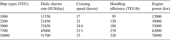
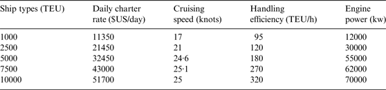
Suppose that there are five types of ships in the network, and the corresponding loading capacity Q are 1000 TEU, 2500 TEU, 5000 TEU, 7500 TEU and 10000 TEU, respectively. According to the Drewry Container Market Quarterly Report of 2007, the parameters of different container ships are selected referring to Table 2. Ship's standby time for departure or arrival at each port (f i , fj ) is supposed to be two hours each. The port related costs such as handling and port entry costs vary from port to port. For simplicity, referring to Shintani et al. (Reference Shintani, Imai, Nishimura and Papadimitriou2007), the handling cost and the cost per entry at each port are 300 $US/TEU and 1·95 × Q + 5200 ($US per entry), respectively. Fuel and lubricant costs (C Fuel, C Lub) are 170 $US/ton and 1000 $US/ton, and fuel and lubricant consumptions (R Fuel, R Lub) are 1·88 × 10−4 ton/kw/h and 5·36 × 10−6 ton/kw/h, respectively.
Parameters of different containerships.
The model parameters are set by L 25(54) orthogonal array. The values of e corresponding to five node sizes are 18, 16, 21, 35 and 36, and the other parameters are set as α ∈ (0·001, 0·2), β ∈ (0·0001, 0·01), ρ ∈ (0·1, 0·9) and E ∈ (0·1, 500). The model is operated in the environment of Intel Core2 Q6600@2.40GHz/3.25GB-DDR2-800/Windows XP SP3, using a steering vector search pattern and random search pattern respectively to calculate the optimal scheme of the networks of five different sizes. Each scale had 100 runs, and the calculation results were collected.
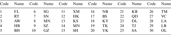
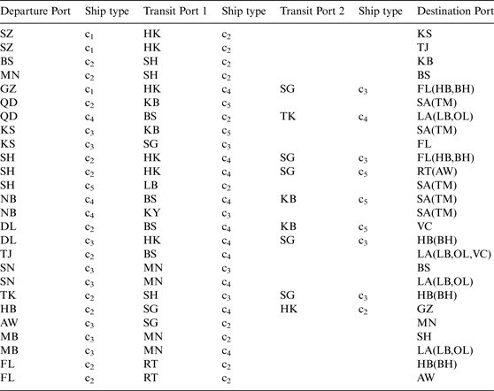
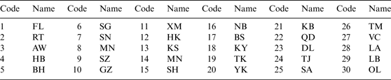
We use the scenario of 30 port nodes under a steering vector search pattern as an example to illustrate the optimisation results. For convenience, port name instead of node code are used, as shown in Table 3. It takes 3·55 hours to obtain the optimisation solution, and the total cost of this scenario is 6362 US$ million. Compared with the total cost of direct shipping (6814·84 US$ million), the gain from the adoption of transhipment is about 6·90%. Table 4 lists the optimisation solution of the container transhipment scheme and direct shipping is adopted for the ODs not listed in the table. It can be seen from Table 4 that ports SG, HK, BS, MN and KB etc. are turned into hub ports, and they collect containers from and distribute containers to other ports in the network. Ship types of 7500 TEU and 10000 TEU are deployed between the hub ports while small ships are deployed for feeder lines for economic benefit.
Port node code and the corresponding name.
Optimisation solution of container transhipment scheme under node scale of 30 ports using steering vector search pattern.

Note: c1-1000 TEU; c2-2500 TEU; c3-5000 TEU; c4-7500 TEU; c5-10000 TEU.
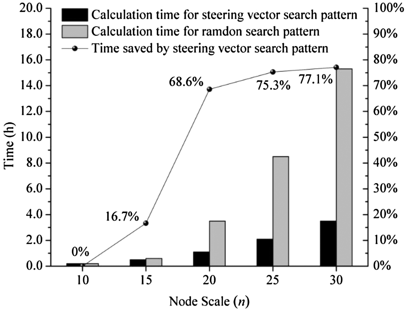
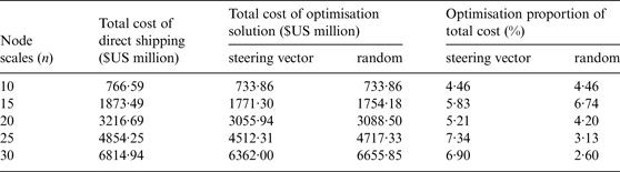
Table 5 and Figure 6 list comparisons of container shipping network optimisation results for steering vector search pattern and random search pattern under five node scales. It can be seen from Table 5 that for the network of large node scales (n = 20, 25 and 30), the steering vector search pattern obtained a better solution than the random search pattern. However, for the network of small node scales, the random search pattern obtained the same solution and achieved an even better solution when n = 10 and n = 15. It is reasonable since the solution obtained in this paper is a convergent solution, not an optimal solution. It can be seen from Figure 6 that for the network of arbitrary node scale, the optimisation algorithm always has a faster convergence with the help of the steering vector. With the increased number of nodes in the random search pattern, the speed of optimisation shows a significant downward trend. It is indicated that for most maritime networks which usually contain a large number of ports, using the steering vector search pattern can effectively improve the efficiency and accuracy of optimisation, and the level of improvement grows significantly with the increase of network scale.
A comparison of searching speed for steering vector and random search pattern.

Comparisons of maritime network optimisation results under five node scales.

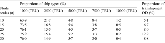
According to the optimisation result of steering vector search pattern, the selection of ship types among the nodes under every type of network size and the proportions of OD choosing transhipment in the network are shown in Table 6.
Comparisons of maritime network optimisation results under five node scales.

Generally, container ships deployed for intercontinental transportation are of large size, while container ships deployed for offshore transportation are of small size. As can be seen from Table 6, most ships used in the network are small size. The possible reason is that most ports are mainly concentrated in several small regions, such as East and Southeast Asia region, West Coast of the US and Mediterranean regions. Due to the short shipment distance, small size ships are preferable for the ports located in the same region. Compared to the large amount of offshore transportation, the rate of intercontinental transportation is relatively small, so most ships in that network are of small size. Generally, to take advantage of the economies of scale for large-scale ships, sufficient cargoes, guarantees of the actual load rate, rationally planned shipping routes, selecting a small group of calling ports, and reducing the port related time are required. Table 6 also shows the vast majority of cargoes adopt direct transport instead of transhipment, because of the high port cost. In the container shipping process, the choice of transit ports should be cautious.
5. DISCUSSIONS AND CONCLUSIONS
To reduce the overall cost of container shipping, rational design of the container shipping network and the deployment of ship types have drawn wide attention from shipping companies. For a large-scale shipping network, traditional algorithms employing random search patterns cannot efficiently solve the optimisation problem of container shipping with transhipments.
Considering the directional property of container shipping routes, this paper improves the traditional ant colony algorithm by introducing the concept of steering vector, and establishes a container shipping network model. The model is solved by the MMAS algorithm based on a steering vector search pattern. Numerical experiments show that steering vector search pattern can reduce search range and calculation time, and increase the number of containable nodes in the model.
The proposed container shipping network optimisation model and the developed solving algorithm will assist liner shipping companies in managing container transportation more economically. Since empty container repositioning is widely-used in real-world container transportation, how to design the container shipping network and deploying container ships by taking into account empty container repositioning is a worthy research topic. Another potential extension is to incorporate stochasticity such as uncertain traffic flow of port pairs to address this problem in a more reliable way.
ACKNOWLEDGEMENTS
This work was supported by the National Natural Science Foundation of China (Grants No. 51279026 & 51309049).