2. Conceptual framework

A considerable body of literature has studied the electoral impact of extreme weather events (Abney and Hill, Reference Abney and Hill1966; Bechtel and Hainmueller, Reference Bechtel and Hainmueller2011; Gasper and Reeves, Reference Gasper and Reeves2011; Reeves, Reference Reeves2011; Chen, Reference Chen2012), the role of political communication in the context of natural disasters (Sood et al., Reference Sood, Stockdale and Rogers1987; Utz et al., Reference Utz, Schultz and Glocka2013), and how public and private actors assess disaster damage when making decisions about their assistance efforts (Waugh and Streib, Reference Waugh and Streib2006; Aldrich, Reference Aldrich2016).Footnote ² So far, however, we do not know which factors drive individual preferences over government responses to natural disasters although they entail the type of divide-the-dollar decisions that figure prominently in formal models of redistribution (Huber and Ting, Reference Huber and Ting2013). However, since disaster relief aims to help individuals who have become victims of a life-threatening, exogenous event, the prominent distinction between luck and effort that the literature on preferences for redistribution tends to emphasize (Durante et al., Reference Durante, Putterman and van der Weele2014; Fisman et al., Reference Fisman, Jakiela, Kariv and Markovits2015; Scheve and Stasavage, Reference Scheve and Stasavage2016) may not offer the most promising theoretical starting point for our conceptual framework. As a consequence, our research question requires us to begin exploring largely unknown territory. However, we can build on existing literature on conceptions of distributive justice (Kendrick, Reference Kendrick1939; Deutsch, Reference Deutsch1975; Lind and Tyler, Reference Lind and Tyler1988), equity and the social contract (Rawls, Reference Rawls2009), and recent theoretical contributions (Valentini, Reference Valentini2013) to develop fairness-based explanations of preferences over the distribution of disaster relief.

When theorizing about how individuals would like to allocate relief aid, an important distributive fairness norm is the ‘polluter-pays’ or ‘affectedness principle'. Whereas the polluter-pays principle applies to situations that require a decision about how to allocate costs, the affectedness principle is relevant when distributing benefits meant to compensate for experienced losses. This fairness norm specifies that the distribution of benefits should be proportional to the experienced losses.Footnote ³ In the context of disaster relief programs, financial benefits are explicitly meant to reflect the level of affectedness by compensating for losses due to a natural disaster. According to the Stafford Act, relief aid is intended “to alleviate the suffering and damage which result from such disasters […] by providing federal assistance programs for both public and private losses sustained in disasters” (Robert T. Stafford Disaster Relief and Emergency Assistance Act, I, Sec. 101, b), (6)). If voters subscribe to affectedness-based fairness we would expect that higher levels of economic damage will increase the amount of relief aid that individuals would like to provide.

Preferences over relief allocations may also be explained by the ability-to-pay principle. This norm, which is most prominent in the context of tax policy questions and “advocated alike by the scholar in taxation and the common man” (Kendrick, Reference Kendrick1939, 92), attempts to determine the amount that constitutes an equal sacrifice when requiring individuals to make a contribution. The ability-to-pay logic can be extended to scenarios that require a distribution of benefits where the allocation would have to account for differences in affluence. When theorizing about how voters judge the provision of disaster relief, this fairness norm suggests that the distribution of relief aid should mirror differences in wealth among disaster victims. Moreover, an important collective goal of relief aid is to help disaster victims recover and this goal may be served best if the allocation of relief aid mirrors the distribution of wealth, as those who are poorer find it more difficult to meet their immediate survival needs and finance economic recovery. Consequently, we expect that individuals prefer to allocate more relief aid to regions that are poorer.

Voters could also view the distribution of policy benefits from a political perspective that highlights the role of electoral reciprocity and partisan solidarity. The electoral reciprocity argument builds on the logic of democratic selection and electoral accountability (Downs, Reference Downs1957). To realize the welfare-enhancing effect of democracy, citizens have to be willing to electorally reward incumbents that have provided them with policy benefits. This incentivizes policymakers to engage in targeted public spending decisions to maximize their re-election chances. While some believe that political leaders tend to pursue universalistic policies, that is, policies that cater to the nation as a whole without favoring particular interests (Cronin and Genovese, Reference Cronin and Genovese2004), others (Kriner and Reeves, Reference Kriner and Reeves2015) have argued that political leaders may engage in partisan particularism by advantaging constituencies that have supported them in the past election.

Clearly, voters could subscribe to the universalistic ideal which requires incumbents to be responsive to all citizens irrespective of whether they have supported the incumbent or not. This argument implies that citizens should not be responsive to electoral considerations when deciding about how to allocate disaster relief. However, individuals could also follow an electoral reciprocity logic. Allocating more relief aid to regions that have voted for the incumbent in previous elections could be seen as an example of political elites giving back to those who have supported them. Even if this concern may be less pronounced than factors such as affectedness or need, voters could place some value on maintaining this reciprocal relationship between affected citizens and the incumbent. If this argument has empirical merit, we would expect that individuals prefer relief allocations that reflect the extent to which an affected county has voted for the incumbent in the previous election.

The partisan solidarity argument highlights that shared partisan orientation could give rise to in-group solidarity. Party identification is not only a stable and powerful predictor of electoral choice and civic engagement (Dalton, Reference Dalton2016), but also offers a shared, loyalty-based identity (Clifford, Reference Clifford2017). This could generate partisan solidarity that gives rise to preferential in-group treatment in which voters who identify with a political party would allocate more relief aid to co-partisans. Our design allows us to test both the electoral reciprocity and the partisan solidarity argument.

3. Data and research design

To empirically evaluate our theoretical predictions, we develop a conjoint experiment (Bechtel and Scheve, Reference Bechtel and Scheve2013; Hainmueller et al., Reference Hainmueller, Hopkins and Yamamoto2014) that asked respondents to make divide-the-dollar decisions (see below). The conjoint experiment was embedded in an online survey fielded to a population-based quota sample of American citizens ($N = 2618$) in December, 2016. The sample was provided by Respondi and based on their online panel. This panel is constructed by drawing a random sample from the population which is then converted into panels and sub-panels on the basis of known population margins (Respondi, Reference Respondi2015). Our survey contains a standard set of sociodemographic questions and several novel question items needed to empirically test the theoretical mechanisms. The full survey instrument is included in the replication archive. The Supplementary Appendix offers detailed information about these questions (Appendix Table A.1) and reports descriptive statistics in Appendix Table A.2. In addition, Appendix Table A.3 shows that the distribution of sociodemographic characteristics in our sample closely matches the population margins. Unless stated otherwise, we report results that employ weights, although the findings remain unchanged when estimated on the unweighted sample.

3.1. Experimental design: relief allocation conjoint and divide-the-dollar decisions

To explore which factors explain individual preferences over the distribution of disaster relief, the conjoint presents respondents with theoretically relevant characteristics of two counties that were affected by a natural disaster. In reality, policymakers (governors and the president) issue county-specific disaster declarations which establish the eligibility of individuals residing in these counties for applying for disaster relief.Footnote ⁴ This turns the distribution of disaster relief into a “divide-the-dollar politics” (Kriner and Reeves, Reference Kriner and Reeves2015) scenario. We mirror this decision by developing a novel outcome measure that asks respondents to split a fixed total amount of relief aid between the affected counties. This modification of the standard conjoint design in combination with county-level scenarios offers two advantages. First, it reflects that budgets are always constrained as this design places a limit on what a respondent can spend in total. Even if disaster relief is often funded by supplemental appropriations, these resources remain ultimately finite. Second, it allows us to perform a more direct comparison between voter preferences and policymakers’ actual relief allocations which are recorded at the county level.

Figure 1 shows the instructions of the conjoint experiment along with the divide-the-dollar outcome question. Our conjoint experiment asks each respondent to distribute a total of $10 million in relief aid between two counties and this task was repeated four times. In total, respondents made 20,944 county-level relief spending decisions. The conjoint contained six dimensions tied to the theoretical expectations: economic damage and the number of fatalities caused by the disaster, average household income, unemployment rate, presidential partisanship, and a county's vote in the 2012 presidential election. For each dimension we used between two and five different values. We detail and justify these dimensions and values below.

Figure 1.

Instructions for the divide-the-dollar conjoint experiment (screenshot). Note: This figure shows the instructions for the conjoint experiment which asked respondents to allocate relief aid between two affected counties. In the conjoint tasks, the values of all attributes were randomized except for presidential partisanship which was randomized across binary comparisons but held constant within each comparison to avoid internally inconsistent hypothetical scenarios. To remove any order effects, the order of the dimensions was randomized across individuals.

3.2. Selection of attribute values in the divide-the-dollar conjoint

Table I presents the attribute values for each dimension. We choose the attribute levels to approximate the historically observed county characteristics as closely as possible. To examine the role of affectedness considerations, we include two attributes that capture the most prominent ways of measuring affectedness: economic damage ($100,000, $1 million, $4 million, $24 million) and the number of fatalities (0, 5). While it is possible for respondents to fully compensate the economic damage whenever disaster losses are $4 million or less, we intentionally include one higher damage level ($24 million) that exceeds the available budget. The purpose of this design is to actually observe individual allocation decisions under a more difficult, but also potentially more realistic scenario in which the available resources are not sufficient to compensate the experienced damage in full. The robustness section reports results suggesting that the structure of mass preferences over disaster relief are quite stable even if the available resources only allow for compensating a fraction of the financial losses.

Table 1.

Distributions of explanatory variables (historical data) and attribute levels for the relief allocation conjoint experiment

Note: This table shows the dimensions and values used in the conjoint experiment. Ranges for economic damage, fatalities, income, and unemployment rate are based on the 25, 50, and 75 percentile of the empirical distributions of these variables in the historical data. All values are randomly assigned except for presidential partisanship which varies randomly between conjoints, but is constant for a given conjoint. $\Delta _v$ denotes the two-party vote share difference in percentage points.

We also include two attributes that measure wealth and need-based characteristics: the average annual household income in a county ($10,000, $40,000, $70,000, $100,000) and the level of joblessness (3, 5, 7, 9 percent). Based on data from 1993 to 2008, 25 percent of all counties experienced unemployment rates between 0 and 4 percent. The corresponding value in the conjoint experiment is the 12.5th percentile, which in this case amounts to 3 percent. Due to inflation and income changes we decided to accept slight deviations from the historically observed values to more closely mirror the more recent distribution of those variables. Finally, to estimate the causal effects of electoral and partisan characteristics, we include presidential partisanship (Democratic, Republican) and five two-party vote share levels that distinguish swing (50 percent/50 percent), core (60 percent/40 percent), core stronghold (70 percent/30 percent), opposition (40 percent/60 percent), and opposition stronghold counties (30 percent/70 percent).

The conjoint fully randomizes all values with the exception of those related to presidential partisanship as it would be illogical if this characteristic differed between counties in a contemporaneous setting. Our design avoids such combinations by keeping presidential partisanship constant within each conjoint comparison while randomizing it across conjoint tasks. This means that whenever a respondent considers two affected counties in a divide-the-dollar conjoint task, presidential partisanship is the same for both of these regions. All other attribute values are fully randomized since none of the remaining potential value combinations result in logically inconsistent scenarios. In addition, we randomize the order of the dimensions between respondents to avoid order effects. However, we keep the order of the dimensions constant within respondents to reduce the complexity of the task (Bechtel and Scheve, Reference Bechtel and Scheve2013).

4. Experimental results

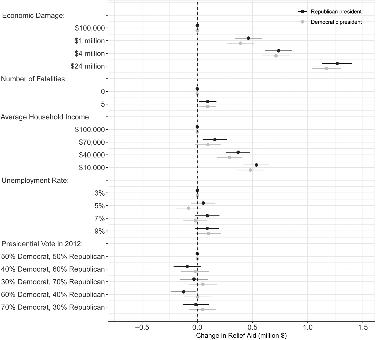
We estimate the causal effects of the conjoint attributes by regressing the amount of relief aid a respondent allocated to a county on treatment variables that indicate the presence or absence of the randomly assigned attribute values for each of the six attributes. Figure 2 reports the causal effects along with 95 percent confidence intervals computed from standard errors clustered by conjoint comparison. Dots without error bars represent the reference categories. Since presidential partisanship was kept constant at the conjoint-task level, we report the results separately by government partisanship. Supplementary Appendix Figure A.1 reports the pooled results using the weighted and unweighted sample. In what follows, we first focus on the causal effects of the conjoint attributes. We then perform various subgroup estimations to evaluate the plausibility of the theoretical mechanisms.

Figure 2.

The causal effects of county characteristics on relief spending preferences by presidential partisanship. This plot shows the causal effects of randomly assigned attribute values on the amount of relief aid allocated to an affected county. Estimates are based on a linear regression of Relief Amount on indicator variables with standard errors clustered by respondent. Horizontal lines indicate 95 percent robust confidence intervals. Points without confidence intervals indicate the reference category for a given attribute. Baseline levels of relief aid: Republican president = $4.1 million, Democratic president = $4.1 million. $N$ (county-level relief spending decisions) = 20,944.

4.2. Theoretical mechanisms

We now explore whether variables related to the underlying theoretical mechanisms systematically moderate the treatment effects in ways consistent with the theory. For example, if affectedness-based norms of distributive justice drive allocation preferences, we would expect the causal effect of economic damage to be stronger among individuals subscribing to an affectedness-based conception of justice. To implement an empirical test of each of the theoretical mechanisms we collect information about whether individuals subscribe to fairness ideas related to affectedness, need, and political ties. We use this data to reestimate the causal effects of county characteristics by theoretically meaningful subgroups. To avoid priming a specific sensitivity among respondents to the attributes included in our relief aid conjoint, these measures of individuals’ fairness norms came after the conjoint experiment. In the robustness section we report additional results that rely on recoded reference categories for these subgroup estimations. Our findings remain unchanged.

4.2.1. Affectedness

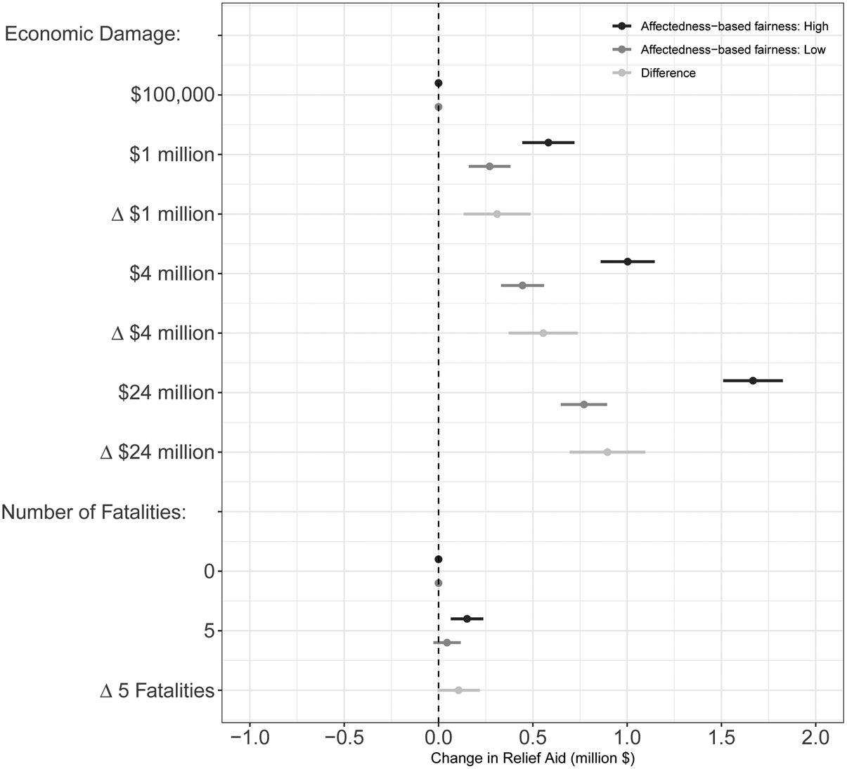
Figure 3 shows the causal effects separately for the group of respondents that are relatively more supportive of affectedness-based fairness and the group of respondents that are less supportive of this conception of justice. This split is based on the question: “People sometimes experience negative events and go through difficult times. To what extent do you agree or disagree (1–10) with the following statement: ‘Those who are more strongly affected should receive more help than those who are less affected’.” This direct question approach seems preferable since—to the best of our knowledge—established and validated indirect measures of the types of fairness norms in which we are interested do not yet exist. Therefore, if we had designed a novel indirect question the results would not have been very informative.Footnote ⁵ We also note that the question wording does not make any reference to the attribute names used in the conjoint (e.g., economic damage, fatalities, etc.). To avoid priming respondents in a specific direction, this question was asked later in the survey. Moreover, the conjoint and the questions regarding support for different types of fairness principles were separated by several question items on other issues. As Supplementary Appendix Table A.2 reports, the median response on this question is 8 which indicates that half of our respondents are quite supportive of an affected-based conception of fairness given that the underlying response scale ranges from 1 (completely disagree) to 10 (completely disagree). We convert respondents’ answers into a binary indicator based on the median that is 1 for those whose level of agreement with the statement was greater than the median, and is zero otherwise. Supplementary Appendix Table A.4 reports the full estimation results for all attributes.

Figure 3.

The causal effects of economic damage and fatalities on relief spending preferences by affectedness-based fairness. This plot shows the causal effects of randomly assigned attribute values on the amount of relief aid allocated to an affected county. Estimates are based on a linear regression of Relief Amount on indicator variables with standard errors clustered by respondent. $\Delta$ reports the difference in the treatment effects between a given attribute level and the reference group. Horizontal lines indicate 95 percent robust confidence intervals. Points without confidence intervals indicate the reference category for a given attribute. Baseline levels of relief aid: Affectedness-based fairness: High = $3.7 million, Affectedness-based fairness: Low = $4.3 million. $N$(county-level relief spending decisions) = 20,944. $N$(respondents) per group = 1,309. The measure of support for affectedness-based fairness is based on the question: “People sometimes experience negative events and go through difficult times. To what extent do you agree or disagree with the following statement: ‘Those who are more strongly affected should receive more support than those who are less affected’.” Respondents’ answers on a 1–10 scale were converted into a binary indicator based on the median. The indicator variable is 1 for those whose level of agreement with the statement was greater than the median and is zero otherwise. Supplementary Appendix Table A.4 reports the full estimation results for all attributes.

The results suggest that respondents who are more supportive of a general affectedness-based fairness norm are much more sensitive to the level of economic losses when allocating relief aid. For example, damage in the order of $4 million increases relief aid by $500,000 among individuals who are relatively less supportive of affectedness-based justice. In contrast, the same amount of economic damage increases relief spending allocated to a county by close to $1 million. Thus, the treatment effect doubles for respondents who are more supportive of affectedness-based justice.

We formally test the hypothesis that the treatment effects for the two groups are statistically different from each other by computing effect differences along with the corresponding 95 percent confidence intervals based on the corresponding variance–covariance matrix. Figure 3 reports these results. We find that respondents who are generally more supportive of affectedness-based fairness provide counties that have experienced $1 million in damage with about $300,000 more relief aid than individuals who are less supportive of this fairness norm. We find similar patterns when examining the effects of higher levels of economic damage. In fact, the difference between the treatment effects becomes larger as disaster damage increases. This heterogeneity in the treatment effects is consistent with the argument that an affectedness-based norm of distributive justice may explain individuals’ strong sensitivity to economic damage when allocating relief aid. Figure 3 also shows that we estimate a significant and positive difference when comparing the causal effect of five fatalities on relief preferences among Affectedness-based fairness: High respondents and Affectedness-based fairness: Low respondents. This suggests that individuals who advocate affectedness-based justice in the abstract tend to provide more relief aid to counties that experienced casualties than respondents who are less supportive of this notion of justice.

4.2.2. Need

Our main results indicate that voter preferences over disaster relief are sensitive to income differences between affected counties. To explore whether this pattern can be explained by a need-based norm of distributive justice, we again use direct question wording that seeks to measure general agreement with this norm while at the same time avoiding any of the terms used in the conjoint attributes: “People sometimes experience negative events and go through difficult times. To what extent do you agree or disagree with the following statement: ‘Those who are richer should receive less support than those who are poorer even if they are equally affected.'” We again split the sample at the median and reestimate the causal effects for both subgroups.Footnote ⁶

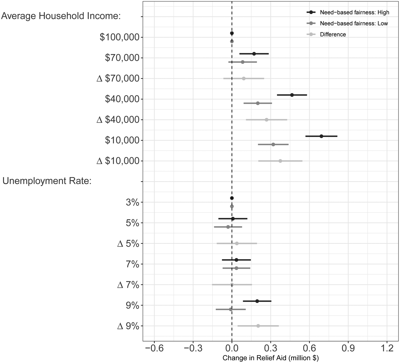
Figure 4 shows the causal effects of need-related factors on the amount of relief aid allocated to a county by our respondents separately for the two groups. We find that the effects of a county's average household income are much stronger among individuals who generally support a need-related notion of distributive justice. For example, individuals subscribing to need-based justice allocate $300,000 more in relief aid to counties with an average household income of $40,000 than individuals who are less supportive of this type of fairness. The heterogeneity in the treatment effects is even larger for very poor counties ($10,000 average household income). Are these effects significantly different from each other when comparing the two groups? Our estimate of the difference in the effects, $\Delta$, which we report with the corresponding 95 percent confidence interval, suggests that this is the case, as the confidence interval excludes zero. These results support the argument that the sensitivity to a county's level of wealth is driven by a need-based notion of distributive justice.

Figure 4.

The causal effects of household income and unemployment on relief spending preferences by need-based fairness. This plot shows the causal effects of randomly assigned attribute values on the amount of relief aid allocated to an affected county. Estimates are based on a linear regression of Relief Amount on indicator variables with standard errors clustered by respondent. $\Delta$ reports the difference in the treatment effects between a given attribute level and the reference group. Horizontal lines indicate 95 percent robust confidence intervals. Points without confidence intervals indicate the reference category for a given attribute. Baseline levels of relief aid: Need-based fairness: High = $4 million, Need-based fairness: Low = $4.2 million. $N$(county-level relief spending decisions) = 20,944. $N$(respondents) per group = 1,309. The measure of support for affectedness-based fairness is based on the question: “People sometimes experience negative events and go through difficult times. To what extent do you agree or disagree with the following statement: ‘Those who are richer should receive less support than those who are poorer even if they are equally affected.’” Respondents’ answers on a 1–10 scale were converted into a binary indicator based on the median. The indicator variable is 1 for those whose level of agreement with the statement was greater than the median and is zero otherwise. Supplementary Appendix Table A.4 reports the full estimation results for all attributes.

When examining the effects of a county's economic standing in terms of joblessness, we find that individuals respond very similarly unless the unemployment rate reaches 9 percent. Given high levels of unemployment, respondents that favor need as a criterion for distributive fairness allocate about $150,000 more in relief payments than individuals less supportive of need-based justice. The difference between those two effects fails to reach significance at the 5 percent level, although it is significant at the 10 percent level.

4.2.3. Political ties: electoral reciprocity and partisan solidarity

A third explanation for voter preferences over relief aid allocations focuses on the role of political ties. If the electoral reciprocity argument is valid, we would expect voters who are more sympathetic toward this fairness norm to allocate more relief aid to counties that have supported the president's party in the previous election. We offer an evaluation of this prediction by first classifying respondents based on their agreement with the statement: “Governments should prioritize the needs of those who voted for them.” The question was asked after the divide-the-dollar conjoint and was separated by a set of items that elicited individuals’ views on other topics. Respondents’ answers on a 1–10 scale were converted into an indicator variable based on the median response.Footnote ⁷ We then further partition our data according to whether the conjoint specified a scenario in which a Democratic or a Republican president was in power. Figures 5A and B report the causal effects along with the differences in the treatment effects ($\Delta$). The estimates reported in Figure 5A indicate that high electoral reciprocators do not systematically allocate more relief aid to Democratic strongholds under a Democratic administration. If anything, such respondents tend to allocate somewhat less relief aid to counties that provided more support for either candidate in the past election, which is inconsistent with the electoral reciprocity argument. We find a similar pattern when exploring respondents’ relief allocations in conjoint scenarios that featured a Republican president.

Figure 5.

The causal effects of previous presidential vote on relief spending choices by electoral reciprocity and government partisanship. (a) Democratic President. (b) Republican President. This plot shows the causal effects of randomly assigned attribute values on the amount of relief aid allocated to an affected county. Estimates are based on a linear regression of Relief Amount on indicator variables with standard errors clustered by respondent. Points without confidence intervals indicate the reference category for a given attribute. $\Delta$ reports the difference in the treatment effects between a given attribute level and the reference group. Horizontal lines indicate 95 percent robust confidence intervals. Baseline levels of relief aid: electoral reciprocity low and Republican president $=$ $3.9 million, electoral reciprocity high and Republican president $=$ $4.3 million, electoral reciprocity low and Democratic president $=$ $3.9 million, electoral reciprocity high and Democratic president $=$ $4.4 million. $N$(county-level relief spending decisions) $=$ 20,944. N(respondents) per group = 1,309.

An alternate version of the political ties argument assumes that respondents’ hold in-group views based on partisanship which could give rise to solidarity among co-partisans. Individuals who identify with a specific party would then allocate more relief aid to regions that are core supporters of their preferred party. To evaluate this argument we break down the results by respondents’ partisan identification and government partisanship. The causal effects of a county's presidential vote reported in Figure 6 indicate that Democratic respondents have a slight preference for favoring Democratic strongholds under a Democratic administration. Republicans do not seem to systematically favor Republican strongholds during times of Republican government partisanship. Overall, the results indicate that even when focusing on political scenarios that should give rise to allocation behavior consistent with partisan solidarity, affectedness and need seem to remain the main concerns.

Figure 6.

The causal effects of county characteristics on relief spending preferences by respondents’ partisan identification and government (presidential) partisanship. This plot shows the causal effects of randomly assigned attribute values on the amount of relief aid allocated to an affected county. Estimates are based on a linear regression of Relief Amount on indicator variables with standard errors clustered by respondent. Horizontal lines indicate 95 percent robust confidence intervals. Points without confidence intervals indicate the reference category for a given attribute. Baseline levels of relief aid: Republican with a Republican president = $4.1 million, Democrat with a Democratic president = $4 million. $N$(county-level relief spending decisions) = 20,944. $N$(respondents) = 2,618.

5. Robustness

We subject our results to a large set of robustness tests which Supplementary Appendix I reports in detail. First, we explore whether the disaster relief preferences of likely voters differ from those of the rest of the adult population. The results in Supplementary Appendix Figure A.2 indicate that this is not the case. Second, we test if voters’ sensitivities depend on whether the available resources are sufficient to fully compensate for experienced disaster losses. We re-estimate the results for the subset of allocation decisions in which the combined damage in both divide-the-dollar conjoint scenarios was equal to or less than $10 million. As the results in Supplementary Appendix Table A.6 show, the structure of mass preferences over disaster relief remains quite comparable to the main results reported above. Preferences may be shaped by personal exposure to extreme weather events. Supplementary Appendix Figure A.3 suggests, however, that the causal effects do not depend on whether a respondent has been personally affected by a natural disaster in the past ten years or not. We find a similar level of homogeneity across levels of attentiveness (Supplementary Appendix Figure A.4) and time spent on the survey (Appendix Figure A.5). We also explore the existence of racial differences in how voters judge the policy responses to natural disasters. The results in Supplementary Appendix Figure A.6 suggest that relief allocations of white and non-white respondents are equally sensitive to economic damage and household income. Moreover, the structure of voter preferences over disaster policy responses are quite stable across different regions (see Supplementary Appendix Figure A.7). We also find that the results are not sensitive to which attribute level is used as the reference category (see Supplementary Appendix Table A.7).

6. Comparing voter preferences over relief spending with observed relief allocations

An important question in research on democratic representation asks whether redistributive spending choices made by public officials correspond to citizens’ preferences. Our data allow us to perform a novel and unusually direct juxtaposition of the structure of voter preferences and policymakers’ actual spending decisions. Clearly, the coefficients from our experimental results and those based on the historical data should not be compared as precisely as two models estimated on the same data. Yet, they offer useful information about whether the empirical patterns are broadly consistent with each other. For this comparison we collect county-level data from the Consolidated Federal Funds Report (CFFR) from 1993 to 2008 and identify those spending items that are related to natural disasters. Supplementary Appendix Tables A.8 and A.9 provide a detailed list of these programs. Our outcome of interest is the amount of relief spending received by a county during a presidential term.Footnote ⁸ This type of temporal aggregation is necessary to evaluate explanations related to government partisanship. We combine these data with information about the occurrence, damage, and associated fatalities of natural disasters from the Spatial Hazard Events and Losses Database for the United States.Footnote ⁹ As others have argued (Kriner and Reeves, Reference Kriner and Reeves2015), there exist many opportunities for elected officials to affect the allocation of relief aid. These include appointing bureaucrats with similar political orientations as well as strategically crafting budget proposals that facilitate electorally profitable spending decisions.

We regress ${{\rm Relief\ Aid}}_{c, t}$ received by county $c$ in term $t$ in logs per capita on covariates that capture need-based, affectedness-based, and electoral considerations.Footnote ¹⁰ Since the outcome variable is log-transformed, the coefficients measure changes in percent (not percentage points). Our predictor variables closely mirror the attributes used in our conjoint experiment. We quantify affectedness in terms of both economic damage and human losses. Damage measures the value of economic damage a county has experienced due to natural disasters in millions of dollars. Fatalities counts the number of individuals who were killed by a disaster. To account for need-based considerations, Household Income measures the average household income in the county and Unemployment Rate is the county-level share of unemployed individuals. To explore the importance of electoral motivations we classify counties into core, core stronghold, swing, opposition, and opposition stronghold counties based on the two-party vote share difference in the previous presidential election.Footnote ¹¹ All regressions include county and period fixed effects, and a set of time-varying sociodemographic and political covariates.

Figure 7 shows the results. We find that disaster damage significantly and positively correlates with the amount of federal relief aid. Compared to the reference group (Economic Damage$\lt$$401,000), counties that experienced losses between $2 and $11 million receive about 25 percent more relief payments. The results also suggest that the allocation of relief aid mirrors the number of casualties. Counties that suffered human losses receive 20 percent more financial support than counties without fatalities. This patterns seem broadly consistent with the structure of voter preferences over the distribution of relief aid.

Figure 7.

Observed and preferred disaster relief allocations. Note: This plot reports linear regression coefficients. Horizontal lines indicate 95 percent robust confidence intervals. For the observed relief allocation results, the dependent variable is the natural logarithm of relief aid received. This model uses county-fixed effects and standard errors clustered at the county level. Controls include preparedness spending as well as socio-economic and political characteristics. Points without confidence intervals indicate the reference categories. The preferred allocation results are based on the main conjoint estimates. $N$ = 12,424.

The estimates reported in Figure 7 also suggest that poorer regions receive more relief aid which is consistent with a need-based fairness norm that also seems to help explain voter preferences over the allocation of disaster assistance. In contrast, we find strongly divergent patterns when examining the correlation between a county's previous voting record and the amount of relief aid it receives. For example, core stronghold counties receive 40 percent more relief payments than observably similar swing states while opposition strongholds on average receive 40 percent less relief aid. The former finding is consistent with the core voter model (Cox, Reference Cox, Shapiro, Stokes, Wood and Kirshner2010) which argues that rewarding loyalists offers additional advantages over an allocation that targets swing voters because of its mobilizing and coordination-enhancing effect. The result is also in line with previous empirical work on the relationship between federal grant aid and a county's historical voting record (Kriner and Reeves, Reference Kriner and Reeves2015).