1 Introduction
Stability is as essential to flight as lift itself. Flyers, living and non-living, are often faced with perturbations in their environment. After a perturbation, a stable flyer returns to its previous orientation passively. An unstable one requires active control (Vogel Reference Vogel2009). The issues of stability and control were indispensable to the development of man-made aircrafts (Wright & Wright Reference Wright and Wright1906) and are pertinent to both the origin of animal flight and the subsequent evolution of flying lineages (Vogel Reference Vogel2009).
The intrinsic stability of flying organisms varies across species. Most birds and insects sacrifice intrinsic stability for gains in manoeuvrability and performance (Vogel Reference Vogel2009; Huang, Nitsche & Kanso Reference Huang, Nitsche and Kanso2015). This trade-off is enabled by sensory feedback and neuromuscular control mechanisms. To identify the sensory circuits and control strategies employed by insects, several approaches have been used. This includes pioneering behavioural experiments as well as anatomical and aerodynamic studies (Fry, Sayaman & Dickinson Reference Fry, Sayaman and Dickinson2003; Taylor & Krapp Reference Taylor and Krapp2007; Ristroph et al. Reference Ristroph, Bergou, Ristroph, Coumes, Berman, Guckenheimer, Wang and Cohen2010; Sun Reference Sun2014).
Insects have also been a source of inspiration for building miniature flying machines; see, for example, Ma et al. (Reference Ma, Chirarattananon, Fuller and Wood2013), Graule et al. (Reference Graule, Chirarattananon, Fuller, Jafferis, Ma, Spenko, Kornbluh and Wood2016), Chen et al. (Reference Chen, Wang, Helbling, Jafferis, Zufferey, Ong, Ma, Gravish, Chirarattananon, Kovac and Wood2017) and references therein. Most designs imitate the flapping motions of insect wings. The aerodynamics of these flapping motions has been clarified by numerous experimental and computational models; see, for example, Ellington et al. (Reference Ellington, van den Berg, Willmott and Thomas1996), Dickinson, Lehmann & Sane (Reference Dickinson, Lehmann and Sane1999), Sane (Reference Sane2003), Wang, Birch & Dickinson (Reference Wang, Birch and Dickinson2004), Wang (Reference Wang2005) and references therein. However, stabilization and control of such biomimetic machines remains a challenge; it requires fast responses to unsteady aerodynamics at small length scales. It is therefore advantageous to invent new engineering designs that are intrinsically stable. To this end, Ristroph & Childress (Reference Ristroph and Childress2014) proposed a jellyfish-inspired machine that required no feedback control to achieve stable hovering and vertical flight. The aerodynamic principles underlying this stable hovering are fundamentally linked to a previous experimental model by the same research team where a pyramid-shaped object pointing upward was shown to hover and maintain balance passively, without internal actuation, in vertically oscillating airflows of zero mean (Childress, Vandenberghe & Zhang Reference Childress, Vandenberghe and Zhang2006; Weathers et al. Reference Weathers, Folie, Liu, Childress and Zhang2010; Liu et al. Reference Liu, Ristroph, Weathers, Childress and Zhang2012). Building on these efforts, Huang et al. (Reference Huang, Nitsche and Kanso2015), Huang, Nitsche & Kanso (Reference Huang, Nitsche and Kanso2016) analysed the aerodynamics and stability of the pyramid-shaped flyer using a two-dimensional computational model based on the inviscid vortex sheet method. Fang et al. (Reference Fang, Ho, Ristroph and Shelley2017) applied a similar approach to examine the stability of the jellyfish-inspired hovering machine. Details of the vortex sheet method can be found in Krasny (Reference Krasny1986), Nitsche & Krasny (Reference Nitsche and Krasny1994), Jones (Reference Jones2003), Jones & Shelley (Reference Jones and Shelley2005), Shukla & Eldredge (Reference Shukla and Eldredge2007), Alben (Reference Alben2009).
Stable hovering in oscillating flows of zero-mean velocity is enabled by the pyramid’s geometric asymmetry and the unsteady vortex structures shed from its outer edges. Liu et al. (Reference Liu, Ristroph, Weathers, Childress and Zhang2012) combined experimental observations with a quasi-steady force theory to estimate the effect of this asymmetry without ever solving for the coupled fluid–flyer interactions. They reported that, contrary to intuition, pyramids with higher centre of mass are more stable. Coupled fluid–flyer interactions were computed by Huang et al. (Reference Huang, Nitsche and Kanso2015, Reference Huang, Nitsche and Kanso2016) in the context of a two-dimensional
 $\wedge$
-shaped flyer free to undergo translational and rotational motions in oscillating flows. These computational studies provided valuable insight into the background flow conditions necessary for hovering and into hovering stability. In particular, a transition from stable to unstable, yet more manoeuvrable, hovering was reported as a function of the flyer’s opening angle and background flow acceleration.
As an extension of the research reported in Huang et al. (Reference Huang, Nitsche and Kanso2015), Huang & Kanso (Reference Huang and Kanso2015), Huang et al. (Reference Huang, Nitsche and Kanso2016), we consider here the rotational stability of a heavy
 $\wedge$
-shaped flyer that is attached at its apex, but free to rotate, in a vertically oscillating background flow. As in a simple pendulum, in the absence of flow oscillations, the
 $\wedge$
-configuration is stable and the
 $\vee$
-configuration is unstable. We first consider rigid flyers and examine the stability of these two configurations in oscillating flows using both a vortex sheet model and a quasi-steady point-force model. We then introduce a rotational spring at the apex of the flyer and allow it to flap passively under background flow oscillations. We examine the difference in stability between the rigid and elastic flyers. We conclude by summarizing the main findings of this study and commenting on its utility for directing future research on flight stability.
2 Problem formulation
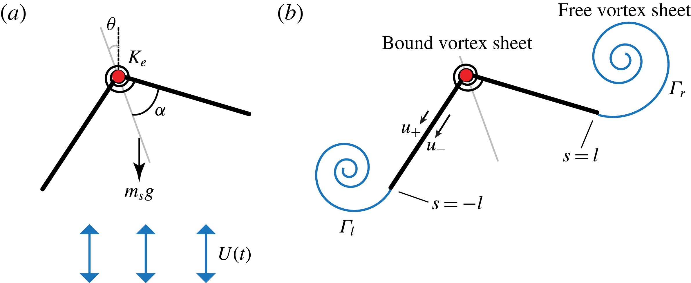
The flyer consists of two flat ‘wings’ connected rigidly at their apex to form a
 $\wedge$
-flyer, as shown in figure 1(a). The opening angle of the flyer is
 $2\unicode[STIX]{x1D6FC}$
. The wings are made of rigid plates of homogeneous density
 $\unicode[STIX]{x1D70C}_{s}$
, length
 $l$
and thickness
 $e$
that is small relative to
 $l$
. The mass per unit depth of each wing is given by
 $m_{s}=\unicode[STIX]{x1D70C}_{s}le$
. The flyer is suspended at its apex
 $O$
but free to rotate about
 $O$
at an angle
 $\unicode[STIX]{x1D703}$
measured counterclockwise from the vertically up direction. The flyer is placed in a background flow of density
 $\unicode[STIX]{x1D70C}_{f}$
oscillating vertically at a velocity
 $U(t)=\unicode[STIX]{x03C0}fA\sin (2\unicode[STIX]{x03C0}ft)$
with zero mean. Here,
 $f$
is the oscillation frequency and
 $A$
is the peak-to-peak amplitude.
(a) Schematic of the two-dimensional
 $\wedge$
-shaped flyer in oscillatory fluid. (b) Depiction of the vortex sheet model used for calculating the aerodynamic forces and torques on the flyer.

The equation governing the rotational motion of the flyer is obtained from the conservation of angular momentum about point
 $O$
of the two-wing system subject to gravitational and aerodynamic effects,
 $$\begin{eqnarray}{\textstyle \frac{2}{3}}m_{s}l^{2}\ddot{\unicode[STIX]{x1D703}}=-(m_{s}-m_{f})gl\cos \unicode[STIX]{x1D6FC}\sin \unicode[STIX]{x1D703}+T_{1}+T_{2}.\end{eqnarray}$$
Here,
 $g$
is the gravitational constant,
 $m_{f}=\unicode[STIX]{x1D70C}_{f}le$
is the mass of displaced fluid and
 $(m_{s}-m_{f})g$
is the net weight of each wing counteracted by the buoyancy effects. The aerodynamic torques on the left and right wings respectively are denoted by
 $T_{1}$
and
 $T_{2}$
, resulting in a total aerodynamic torque
 $T=T_{1}+T_{2}$
about the flyer’s point of suspension
 $O$
. If these torques were zero, (2.1) reduces to the equation
 $\ddot{\unicode[STIX]{x1D703}}=-(g/l_{p})\sin \unicode[STIX]{x1D703}$
governing the rotational motion of a simple pendulum of length
 $l_{p}=(2m_{s}/3(m_{s}-m_{f}))(l/\text{cos}\,\unicode[STIX]{x1D6FC})$
.
For the flexible flyers, we introduce elasticity into the model in the form of a torsional spring of stiffness
 $K_{e}$
placed at the base point connecting the two rigid wings. For this case, in addition to the rotational dynamics in (2.1), the shape of the flyer, represented by the half-opening angle
 $\unicode[STIX]{x1D6FC}$
, changes in time. The equation of motion governing the shape evolution is obtained by balancing the angular momentum for each wing separately and subtracting the resulting two equations. This yields
 $$\begin{eqnarray}{\textstyle \frac{2}{3}}m_{s}l^{2}\ddot{\unicode[STIX]{x1D6FC}}=-(m_{s}-m_{f})gl\sin \unicode[STIX]{x1D6FC}\cos \unicode[STIX]{x1D703}-(T_{1}-T_{2})-4K_{e}(\unicode[STIX]{x1D6FC}-\unicode[STIX]{x1D6FC}_{r}).\end{eqnarray}$$
Here,
 $\unicode[STIX]{x1D6FC}_{r}$
is the rest half-angle of the torsional spring.
Dimensional versus dimensionless quantities. The dimensionless ranges considered here lie within observed values for insects and small birds in dimensional terms. Constant parameters are
 $\unicode[STIX]{x1D70C}_{f}=1.225~\text{kg}~\text{m}^{3}$
,
 $g=9.81~\text{m}~\text{s}^{-1}$
. Wing thickness-to-length ratio is assumed to be
 $e/l=0.01$
.

To make the equations of motion (2.1) and (2.2) dimensionless, we scale length by
 $l$
, time by
 $1/f$
and mass by the wing’s added mass
 $\unicode[STIX]{x1D70C}_{f}l^{2}$
. The number of independent parameters is then reduced to five dimensionless quantities: the amplitude
 $\unicode[STIX]{x1D6FD}$
and acceleration
 $\unicode[STIX]{x1D705}$
of the background flow and the mass
 $m$
, rest angle
 $\unicode[STIX]{x1D6FC}_{r}$
and stiffness
 $k_{e}$
of the flyer,
 $$\begin{eqnarray}\unicode[STIX]{x1D6FD}=\frac{A}{l},\quad \unicode[STIX]{x1D705}=\frac{2m_{s}Af^{2}}{3(m_{s}-m_{f})g},\quad m=\frac{2m_{s}}{3\unicode[STIX]{x1D70C}_{f}l^{2}},\quad \unicode[STIX]{x1D6FC}_{r},\quad k_{e}=\frac{4K_{e}}{\unicode[STIX]{x1D70C}_{f}l^{4}f^{2}}.\end{eqnarray}$$
For the rigid flyer,
 $k_{e}=\infty$
and
 $\unicode[STIX]{x1D6FC}=\unicode[STIX]{x1D6FC}_{r}$
for all time. The range of dimensional and dimensionless parameter values used in this study are listed in table 1 and lie within observed values in insects and small birds (Ellington et al.
Reference Ellington, van den Berg, Willmott and Thomas1996; Dickinson et al.
Reference Dickinson, Lehmann and Sane1999; Spedding, Rosén & Hedenström Reference Spedding, Rosén and Hedenström2003; Thomas et al.
Reference Thomas, Taylor, Srygley, Nudds and Bomphrey2004; Warrick, Tobalske & Powers Reference Warrick, Tobalske and Powers2005). Dimensionless counterparts to (2.1) and (2.2) can be written as
 $$\begin{eqnarray}\left.\begin{array}{@{}c@{}}\displaystyle m\ddot{\unicode[STIX]{x1D703}}=-\frac{m\unicode[STIX]{x1D6FD}}{\unicode[STIX]{x1D705}}\cos \unicode[STIX]{x1D6FC}\sin \unicode[STIX]{x1D703}+(T_{1}+T_{2}),\\ \displaystyle m\ddot{\unicode[STIX]{x1D6FC}}=-\frac{m\unicode[STIX]{x1D6FD}}{\unicode[STIX]{x1D705}}\sin \unicode[STIX]{x1D6FC}\cos \unicode[STIX]{x1D703}-(T_{1}-T_{2})-k_{e}(\unicode[STIX]{x1D6FC}-\unicode[STIX]{x1D6FC}_{r}).\end{array}\right\}\end{eqnarray}$$
Here, the aerodynamic torques
 $T_{1}$
and
 $T_{2}$
are considered to be dimensionless. The dimensionless background flow is given by
 $U(t)=\unicode[STIX]{x03C0}\unicode[STIX]{x1D6FD}\sin (2\unicode[STIX]{x03C0}t)$
.
3 The vortex sheet method
We apply an inviscid vortex sheet model to calculate the aerodynamic forces and torques exerted on the flyer by the surrounding fluid. A detailed description of the vortex sheet method can be found in Huang et al. (Reference Huang, Nitsche and Kanso2016) and references therein. Huang et al. (Reference Huang, Nitsche and Kanso2016) presented a careful comparison between the numerical results obtained using our implementation of the vortex sheet model and the results obtained by Jones (Reference Jones2003) and Jones & Shelley (Reference Jones and Shelley2005) for a flat plate. Here, we provide a brief outline of the method. In this treatment, the wing system is modelled as a bound vortex sheet of zero thickness and the vorticity shed at each edge is represented as a free vortex sheet, as shown in figure 1(b). Vorticity is distributed along the free and bound vortex sheets with sheet strength
 $\unicode[STIX]{x1D6FE}(s,t)$
, as a function of the arc length
 $s$
and time
 $t$
. We define the total circulation of the left and right vortex sheets as
 $\unicode[STIX]{x1D6E4}_{l}=\int _{s_{l}}\unicode[STIX]{x1D6FE}(s,t)\,\text{d}s$
and
 $\unicode[STIX]{x1D6E4}_{r}=\int _{s_{r}}\unicode[STIX]{x1D6FE}(s,t)\,\text{d}s$
respectively. Here,
 $s_{l}$
and
 $s_{r}$
are used to denote the arc lengths along the left and right vortex sheets. The distribution of the bound sheet strength at each time step is solved by satisfying the normal boundary conditions on the wings and Kevin’s circulation theorem. The Kutta condition gives the shedding rates at the two outer edges as
 $$\begin{eqnarray}\left.\frac{\text{d}\unicode[STIX]{x1D6E4}_{l}}{\text{d}t}\right|_{s_{b}=-l}=\left.-\frac{1}{2}(u_{-}^{2}-u_{+}^{2})\right|_{s_{b}=-l},\quad \left.\frac{\text{d}\unicode[STIX]{x1D6E4}_{l}}{\text{d}t}\right|_{s_{b}=l}=\left.\frac{1}{2}(u_{-}^{2}-u_{+}^{2})\right|_{s_{b}=l},\end{eqnarray}$$
where
 $s_{b}$
is the arc length along the bound vortex sheet (
 $s_{b}=-l$
and
 $s_{b}=l$
denote the arc lengths of the left and right edges separately) and
 $u_{\pm }$
are the slip velocities above and below the flat wings, namely the tangential velocity difference between the fluid and the wing. Under unfavourable shedding conditions, such as when the background flow opposes vortex shedding (Jones & Shelley Reference Jones and Shelley2005), we halt the shedding of a new vortex element as done in Alben (Reference Alben2010). It is important to point out that no vorticity is shed from the apex; the model therefore ignores some of the physics when shedding from the apex is expected such as when the wedge is oriented orthogonal to the oncoming flow.
Once the vorticity distribution is computed, the pressure difference across the wings can be obtained from Euler’s equation. To this end, we get
 $$\begin{eqnarray}[p]_{+}^{-}(s_{b},t)=p_{-}(s_{b},t)-p_{+}(s_{b},t)=-\frac{\text{d}\unicode[STIX]{x1D6E4}(s_{b},t)}{\text{d}t}-\frac{1}{2}(u_{-}^{2}-u_{+}^{2}),\end{eqnarray}$$
where
 $\unicode[STIX]{x1D6E4}(s_{b},t)=\unicode[STIX]{x1D6E4}_{l}+\int _{-l}^{s_{b}}\unicode[STIX]{x1D6FE}(s,t)\,\text{d}s$
. The fluid force is due to pressure only; the force and torque acting on each wing with respect to the attachment point
 $O$
are given by
 $$\begin{eqnarray}\displaystyle \left.\begin{array}{@{}c@{}}\displaystyle F_{x}=\int _{-l}^{l}[p]_{+}^{-}n_{x}\,\text{d}s,\quad F_{y}=\int _{-l}^{l}[p]_{+}^{-}n_{y}\,\text{d}s,\\ \displaystyle T=\int _{-l}^{l}[p]_{+}^{-}((x_{b}-x_{o})n_{y}-(y_{b}-y_{o})n_{x})\,\text{d}s.\end{array}\right\} & & \displaystyle\end{eqnarray}$$
Here,
 $n_{x}$
and
 $n_{y}$
are the
 $x$
- and
 $y$
-components of the unit vector normal to the wings,
 $(x_{b},y_{b})$
is the position of the bound vortex sheet along the wings, and
 $(x_{o},y_{o})$
is the fixed position of the attachment point. Both
 $(x_{b},y_{b})$
and
 $(n_{x},n_{y})$
are functions of arc length.
To emulate the effect of fluid viscosity, we follow Huang et al. (Reference Huang, Nitsche and Kanso2015, Reference Huang, Nitsche and Kanso2016) and we introduce a dimensionless time parameter
 $\unicode[STIX]{x1D70F}_{diss}$
, such that the point vortices shed at time
 $t-\unicode[STIX]{x1D70F}_{diss}$
are manually removed from the fluid at time
 $t$
. Here, we set
 $\unicode[STIX]{x1D70F}_{diss}=0.6$
. Note that this approach indirectly introduces dissipation because each vortex removal amounts to adding a small dissipative force to the force balance on the wedge. This dissipative force is small, as long as the value of
 $\unicode[STIX]{x1D70F}_{diss}$
is sufficiently far from the oscillation period of the background flow. The dissipative force introduced by the method is quantified for fixed and pitching plates in background flow in the Appendix. A complete description of the variation in dissipation with
 $\unicode[STIX]{x1D70F}_{diss}$
is outside the scope of the present study. However, we note that the value chosen here,
 $\unicode[STIX]{x1D70F}_{diss}=0.6$
, is far from any potential resonances.
Given that the dissipation time imitates viscosity, we anticipate the dimensional dissipation time
 $\unicode[STIX]{x1D70F}_{diss}^{\ast }$
to scale as
 $\unicode[STIX]{x1D70F}_{diss}^{\ast }\sim \unicode[STIX]{x1D6FF}^{2}/\unicode[STIX]{x1D708}$
, where
 $\unicode[STIX]{x1D6FF}$
is the characteristic thickness of the vortex sheet and
 $\unicode[STIX]{x1D708}$
is kinematic viscosity. This scaling argument can be used to obtain an estimate of the Reynolds number,
 $Re=Afl/\unicode[STIX]{x1D708}=Afl\unicode[STIX]{x1D70F}_{diss}^{\ast }/\unicode[STIX]{x1D6FF}^{2}\approx 0.6Al/\unicode[STIX]{x1D6FF}^{2}$
. In our simulations, the regularized thickness of the vortex sheet
 $\unicode[STIX]{x1D6FF}/l$
is of order
 $10^{-2}$
. Consequently, for the range of parameter values listed in table 1, one gets Reynolds numbers ranging from 600 to 6000.
4 Results: rigid flyers
The concave-down (
 $\wedge$
) and concave-up (
 $\vee$
) configurations of the flyer are equilibrium solutions of (2.4). This result follows directly from symmetry about the vertical direction. In the absence of flow oscillations, as in a simple pendulum, the
 $\wedge$
-configuration is stable and the
 $\vee$
-configuration is unstable. Here, we examine the stability of these two configurations in oscillating flows by solving the nonlinear system of equations for the coupled fluid–flyer model. For concreteness, we consider perturbations of the flyer’s initial orientation
 $\unicode[STIX]{x1D703}(0)$
while keeping
 $\dot{\unicode[STIX]{x1D703}}(0)=0$
. For the elastic flyer discussed in § 5, we additionally set
 $\unicode[STIX]{x1D6FC}(0)-\unicode[STIX]{x1D6FC}_{r}=\dot{\unicode[STIX]{x1D6FC}}(0)=0$
.
4.1 Bistable behaviour
We impose non-zero initial perturbations
 $\unicode[STIX]{x1D703}(0)$
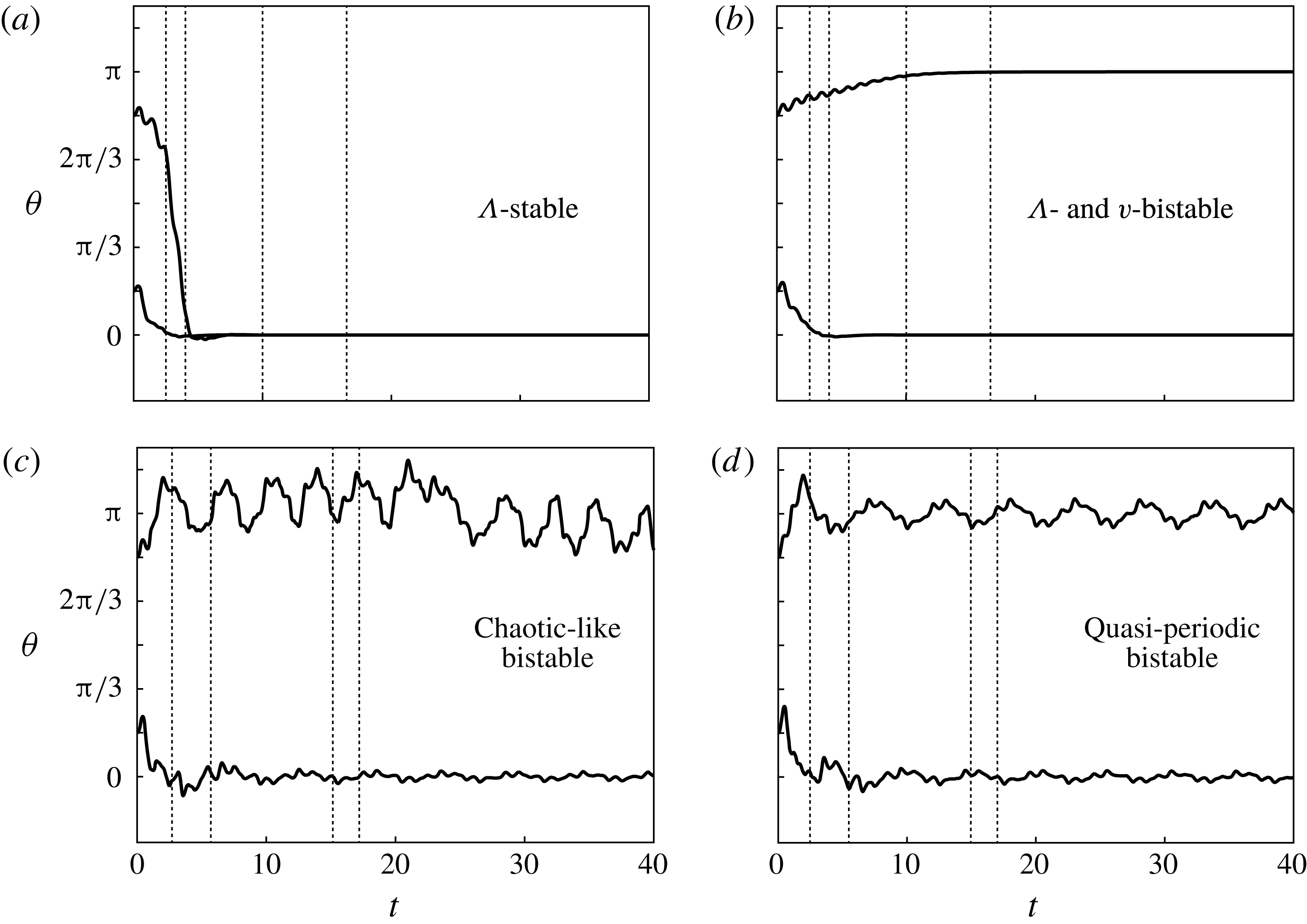
and we solve (2.4), coupled to the vortex sheet model, for each initial perturbation. Figure 2 shows the rotational motion
 $\unicode[STIX]{x1D703}(t)$
of a flyer of mass
 $m=1$
and half-opening angle
 $\unicode[STIX]{x1D6FC}=\unicode[STIX]{x03C0}/6$
for four sets of flow parameters
 $(\unicode[STIX]{x1D6FD},\unicode[STIX]{x1D705})=(0.6,0.15)$
,
 $(0.6,0.3)$
,
 $(1.2,0.15)$
and
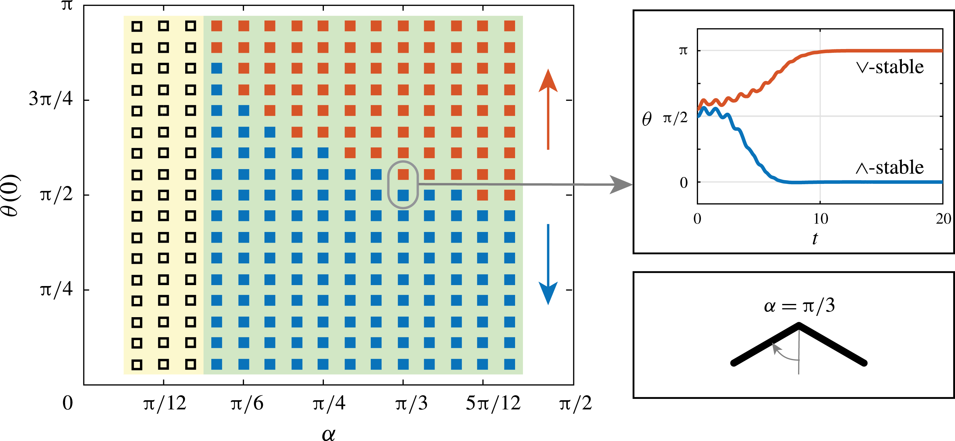
 $(1.2,0.3)$
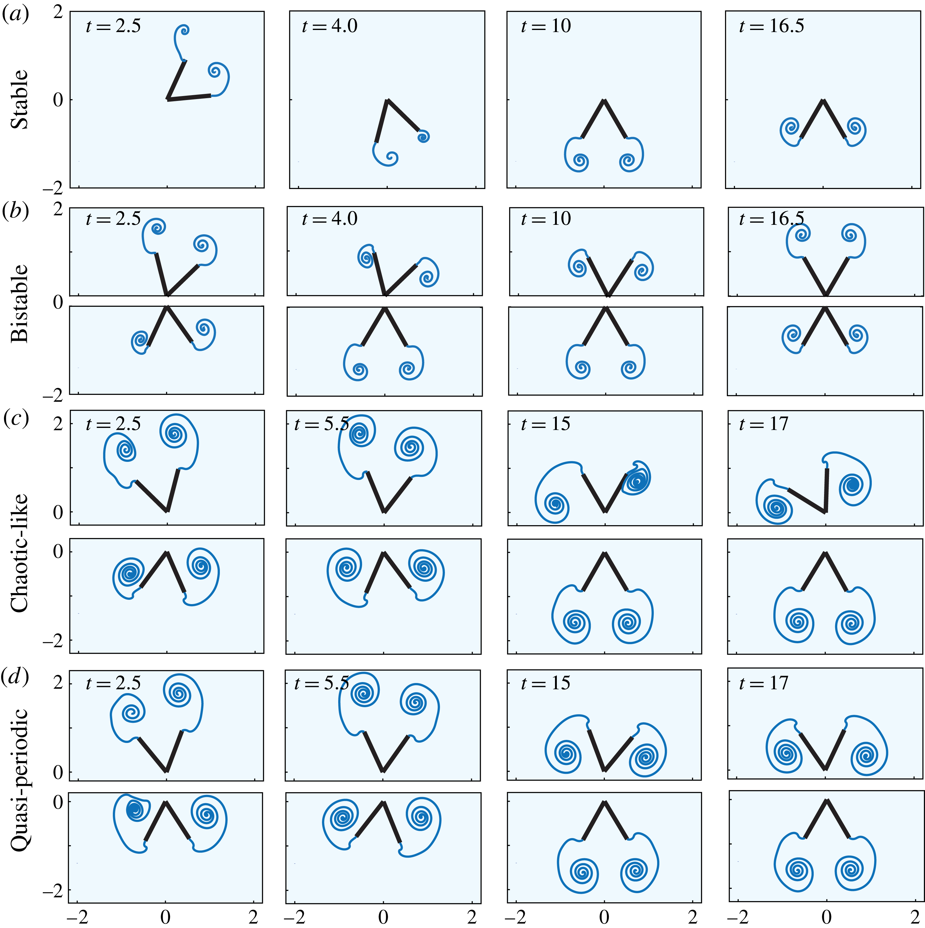
. Figure 3 shows snapshots of the flyer and its unsteady wake for these four cases. Two distinct nonlinear behaviours are observed: stable behaviour where the flyer gravitates to the concave-down
 $\wedge$
-configuration for all initial perturbations (figure 2
a) and bistable behaviour where the flyer tends to either the concave-down
 $\wedge$
- or concave-up
 $\vee$
-configuration depending on the initial perturbation (figure 2
b). We further distinguish three types of bistable behaviour: asymptotically stable behaviour where
 $\unicode[STIX]{x1D703}$
converges to either
 $0$
or
 $\unicode[STIX]{x03C0}$
(figure 2
b), bounded ‘chaotic-like’ oscillations about
 $0$
or
 $\unicode[STIX]{x03C0}$
(figure 2
c) and ‘quasi-periodic’ oscillations about
 $0$
or
 $\unicode[STIX]{x03C0}$
(figure 2
d). Similar bounded oscillations were observed in the stable behaviour about the concave-down
 $\wedge$
-configuration, the time trajectories of which are omitted for brevity.
Rotational behaviour of a rigid flyer (
 $m=1$
,
 $\unicode[STIX]{x1D6FC}=\unicode[STIX]{x03C0}/6$
) in oscillatory flows. Flow parameters are (a)
 $\unicode[STIX]{x1D6FD}=0.6$
,
 $\unicode[STIX]{x1D705}=0.15$
, (b)
 $\unicode[STIX]{x1D6FD}=0.6$
,
 $\unicode[STIX]{x1D705}=0.30$
, (c)
 $\unicode[STIX]{x1D6FD}=1.2$
,
 $\unicode[STIX]{x1D705}=0.15$
and (d)
 $\unicode[STIX]{x1D6FD}=1.2$
,
 $\unicode[STIX]{x1D705}=0.30$
. Initial perturbations are set to
 $\unicode[STIX]{x1D703}(0)=\unicode[STIX]{x03C0}/6$
and
 $\unicode[STIX]{x1D703}(0)=5\unicode[STIX]{x03C0}/6$
. Figure 3 shows snapshots of the flyer’s wake at the time instants highlighted by vertical dashed lines.

Snapshots of the flyers and their wakes at the time instants highlighted by vertical dashed lines in figure 2.

Stabilization of the flyer in the concave-up
 $\vee$
-configuration is fundamentally due to unsteady aerodynamics. Snapshots of the flyers and their unsteady wakes are shown in figure 3. The flyer is subject to gravitational and aerodynamic forces only. The torque
 $-m\unicode[STIX]{x1D6FD}\unicode[STIX]{x1D705}^{-1}\cos \unicode[STIX]{x1D6FC}\sin \unicode[STIX]{x1D703}$
induced by the gravitational force tends to align the flyer with
 $\unicode[STIX]{x1D703}=0$
for all orientations. Thus, it has a destabilizing effect on the concave-up
 $\vee$
-configuration. Later in this paper we analyse the aerodynamic forces
 $F_{x}$
and
 $F_{y}$
and torque
 $T$
acting on the flyer and explain the aerodynamic origin of the bistable behaviour. First, we map the flyer’s stable and bistable behaviour onto the two-dimensional parameter space (
 $\unicode[STIX]{x1D6FD}$
,
 $\unicode[STIX]{x1D705}$
) of flow amplitudes and accelerations.
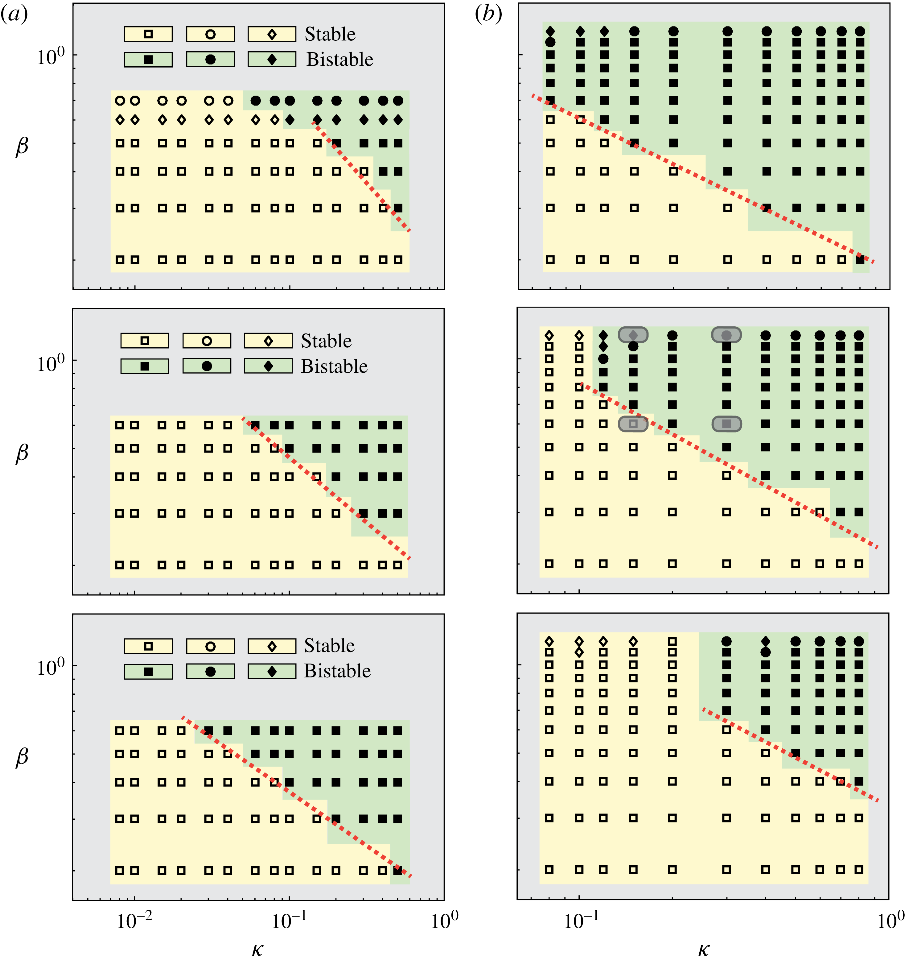
Stable and bistable behaviour of rigid flyers mapped onto the (
 $\unicode[STIX]{x1D705}$
,
 $\unicode[STIX]{x1D6FD}$
) for (a)
 $\unicode[STIX]{x1D6FC}=\unicode[STIX]{x03C0}/12,\unicode[STIX]{x03C0}/6$
and
 $\unicode[STIX]{x03C0}/4$
and
 $m=0.074$
and (b)
 $\unicode[STIX]{x1D6FC}=\unicode[STIX]{x03C0}/6$
and
 $m=0.5,1,2$
. Grey boxes are used to highlight the four sets of parameters used in figure 2. The open symbols ‘▫’ ‘♢’ and ‘○’ correspond to stable concave-down
 $\wedge$
-configuration, with ‘▫’ representing asymptotically stable behaviour (
 $\unicode[STIX]{x1D703}\rightarrow 0$
) and ‘♢’ and ‘○’ representing bounded chaotic-like and periodic oscillations about
 $\unicode[STIX]{x1D703}=0$
, respectively. The filled symbols ‘▪’ ‘♦’ and ‘●’ are used to denote bistable behaviour.

Figure 4 shows the (
 $\unicode[STIX]{x1D6FD},\unicode[STIX]{x1D705}$
)-space in log–log scale for six distinct flyers: three flyers of increasing opening angle
 $\unicode[STIX]{x1D6FC}=\unicode[STIX]{x03C0}/12,\unicode[STIX]{x03C0}/6$
and
 $\unicode[STIX]{x03C0}/4$
and same mass
 $m=0.074$
(figure 4
a), and three flyers of the same angle
 $\unicode[STIX]{x1D6FC}=\unicode[STIX]{x03C0}/6$
and increasing mass
 $m=0.5$
,
 $1$
and
 $2$
(figure 4
b). Specifically, we vary
 $\unicode[STIX]{x1D6FD}$
from
 $0.1$
to
 $1$
and
 $\unicode[STIX]{x1D705}$
from
 $0.01$
to
 $1$
. Stable behaviour about the concave-down
 $\wedge$
-configuration is represented by the open symbols ‘▫’ ‘♢’ and ‘○’, corresponding to asymptotically stable behaviour (
 $\unicode[STIX]{x1D703}\rightarrow 0$
), bounded chaotic-like and periodic oscillations about
 $\unicode[STIX]{x1D703}=0$
, respectively. The filled symbols ‘▪’ ‘♦’ and ‘●’ are used to denote bistable behaviour. The best-fit line for the points at which the transition from asymptotically stable to asymptotically bistable behaviour is first observed is highlighted by a dashed red line, with bistable behaviour observed for values of
 $\unicode[STIX]{x1D6FD}$
and
 $\unicode[STIX]{x1D705}$
values that satisfy
 $$\begin{eqnarray}\unicode[STIX]{x1D6FD}/\unicode[STIX]{x1D705}^{a}>b.\end{eqnarray}$$
The slope
 $a$
of the transition line and threshold value
 $b$
above which the transition occurs depend on the flyer’s shape
 $\unicode[STIX]{x1D6FC}$
and mass
 $m$
, as detailed in table 2. The slope
 $a$
increases as
 $\unicode[STIX]{x1D6FC}$
increases but is relatively insensitive to changes in mass. Meanwhile, the threshold
 $b$
decreases with
 $\unicode[STIX]{x1D6FC}$
but increases with
 $m$
. Taken together, these results indicate that wider flyers, which amplify the aerodynamic torque, tend to transition to bistable behaviour at lower values of flow amplitude
 $\unicode[STIX]{x1D6FD}$
and acceleration
 $\unicode[STIX]{x1D705}$
than narrower flyers. They also indicate that heavier flyers require larger values of
 $\unicode[STIX]{x1D6FD}$
and
 $\unicode[STIX]{x1D705}$
to make this transition.
An estimate of the transition from stable to bistable behaviour can be obtained by noting that upward stability occurs when the aerodynamic torque balances the gravitational torque. Considering a quasi-steady drag formulation, the aerodynamic force in dimensional form is proportional to
 $\unicode[STIX]{x1D70C}_{f}l(Af)^{2}$
and the aerodynamic torque to
 $\unicode[STIX]{x1D70C}_{f}l^{2}(Af)^{2}$
. In dimensionless form, one has
 $T\sim \unicode[STIX]{x1D70C}_{f}l^{2}(Af)^{2}/\unicode[STIX]{x1D70C}_{f}l^{4}f^{2}=\unicode[STIX]{x1D6FD}^{2}$
. From (2.4), the gravitational torque scales as
 $m\unicode[STIX]{x1D6FD}\unicode[STIX]{x1D705}^{-1}\cos \unicode[STIX]{x1D6FC}$
. Thus, the ratio of aerodynamic to gravitational torque is given by
 $\unicode[STIX]{x1D6FD}/\unicode[STIX]{x1D705}^{-1}m\cos \unicode[STIX]{x1D6FC}$
, yielding
 $\unicode[STIX]{x1D6FD}/\unicode[STIX]{x1D705}^{-1}\geqslant m\cos \unicode[STIX]{x1D6FC}$
for upward stability. The threshold to bistability increases with
 $m$
and decreases as
 $\unicode[STIX]{x1D6FC}$
increases from
 $0$
to
 $\unicode[STIX]{x03C0}/2$
, which is consistent with the numerical results in figure 4 and table 1. However, a direct comparison of the condition
 $\unicode[STIX]{x1D6FD}/\unicode[STIX]{x1D705}^{-1}\geqslant m\cos \unicode[STIX]{x1D6FC}$
obtained from such scaling argument with equation (4.1) implies that
 $a=-1$
whereas the values listed in table 1 based on the vortex sheet method lie within
 $-1<a<0$
. This discrepancy indicates that the simple scaling argument based on quasi-steady drag does not quantitatively capture the aerodynamic torques generates by the unsteady flow. This is not too surprising since the quasi-steady scaling arguments presented above essentially assume a constant drag coefficient. In unsteady flows, the effective drag coefficient is known to depend strongly on the ratio
 $\unicode[STIX]{x1D6FD}$
of oscillation amplitude to object size (the so-called Keulegan–Carpenter number proposed in Keulegan & Carpenter (Reference Keulegan and Carpenter1958)). In general, the aerodynamic forces and torques can be decomposed into fast and slow components: the fast component oscillates with the background flow while the slow component is defined as the time average over the fast oscillations. A more complete model for the time-averaged (slow) aerodynamics that describes the origin of the observed bistable behaviour is presented in § 4.6.
Transition from stable to bistable behaviour first occurs at
 $\unicode[STIX]{x1D6FD}/\unicode[STIX]{x1D705}^{a}>b$
where
 $a$
and
 $b$
are obtained from linearly fitting the lower boundary of the bistable (green) region in figure 4.

4.2 Comparison to the inverted pendulum
The bistable behaviour observed here is reminiscent to the behaviour of a classic pendulum undergoing rapid vertical oscillations about its point of suspension, with negligible aerodynamic forces. A classic pendulum of length
 $l_{p}=(2m_{s}/3(m_{s}-m_{f}))(l/\text{cos}\,\unicode[STIX]{x1D6FC})$
equivalent to the submerged flyer can be stabilized about the inverted (vertically up) configuration by an inertia-induced torque provided that the frequency
 $f_{p}$
and amplitude
 $A_{p}$
of the base oscillations satisfy
 $A_{p}^{2}(2\unicode[STIX]{x03C0}f_{p})^{2}>2gl_{p}$
(Butikov (Reference Butikov2001, equation (7))). The inertia-induced torque responsible for this bistability can be best explained in a non-inertial frame of reference that is oscillating with the base point of the pendulum. The acceleration of this frame induces an inertial torque that must be added to the torque of the gravitational force. Such torque is absent in the flyer equations because the flyer’s base point is fixed. To compare the classic pendulum to the flyer, we rewrite the condition
 $A_{p}^{2}(2\unicode[STIX]{x03C0}f_{p})^{2}>2gl_{p}$
for inertia-induced bistability in terms of the dimensionless amplitude
 $\unicode[STIX]{x1D6FD}=A_{p}/l$
and acceleration
 $\unicode[STIX]{x1D705}=(2m_{s}/3(m_{s}-m_{f}))A_{p}f_{p}^{2}/g$
defined according to (2.3); we obtain
 $$\begin{eqnarray}\unicode[STIX]{x1D6FD}/\unicode[STIX]{x1D705}^{-1}>{\displaystyle \frac{1}{2\unicode[STIX]{x03C0}^{2}\cos \unicode[STIX]{x1D6FC}}}\left({\displaystyle \frac{2m_{s}}{3(m_{s}-m_{f})}}\right)^{2}.\end{eqnarray}$$
Comparing (4.1) and (4.2),
 $a$
is always equal to
 $-1$
for the classic pendulum, reinforcing that
 $a$
of the flyer is affected by the flyer’s shape due to aerodynamics. Meanwhile, the threshold
 $b$
for the transition to upward stability depends on both mass and shape, but unlike the trend observed in table 1 for the flyer,
 $b$
for the inverted pendulum increases as
 $\unicode[STIX]{x1D6FC}$
increases from 0 to
 $\unicode[STIX]{x03C0}/2$
.
For a quantitative comparison, consider the flyer with
 $\unicode[STIX]{x1D6FC}=\unicode[STIX]{x03C0}/6$
and
 $m=1$
(middle panel of figure 4
b). The aerodynamic-induced transition occurs for
 $\unicode[STIX]{x1D6FD}/\unicode[STIX]{x1D705}^{-0.57}>0.22$
. If we vary the mass ratio
 $m_{s}/m_{f}$
from 1.2 to 4, the dimensionless quantity
 $(2m_{s}/3(m_{s}-m_{f}))$
decreases from
 $4$
to
 $8/9$
and the threshold value
 $b$
for the inertia-induced transition decreases by an order of magnitude from
 $0.23$
to
 $0.05$
. At
 $m_{s}/m_{f}=1.52$
, the inertia- and aerodynamic-induced transitions have the same value
 $b=0.22$
. In this case, for accelerations
 $0<\unicode[STIX]{x1D705}<1$
, the flyer transitions to upward stability at smaller oscillation amplitude
 $\unicode[STIX]{x1D6FD}$
than the classic pendulum. By the same token, for a given amplitude
 $\unicode[STIX]{x1D6FD}$
, this transition requires smaller
 $\unicode[STIX]{x1D705}$
and consequently smaller oscillation frequency.
Basins of attraction for the (blue) downward
 $\wedge$
- and (red) upward
 $\vee$
-stable configurations for flyers of opening angle
 $\unicode[STIX]{x1D6FC}$
ranging from
 $\unicode[STIX]{x03C0}/18$
to
 $4\unicode[STIX]{x03C0}/9$
by the increment of
 $\unicode[STIX]{x03C0}/36$
. Initial orientation
 $\unicode[STIX]{x1D703}(0)$
increases from
 $\unicode[STIX]{x03C0}/18$
to
 $17\unicode[STIX]{x03C0}/18$
by
 $\unicode[STIX]{x03C0}/18$
while the initial angular velocity is
 $\dot{\unicode[STIX]{x1D703}}(0)=0$
. Parameters are set to
 $m=1$
,
 $\unicode[STIX]{x1D705}=0.5$
, and
 $\unicode[STIX]{x1D6FD}=0.5$
. The open symbols ‘▫’ correspond to stable concave-down
 $\wedge$
-configuration while the filled symbols ‘▪’ denote bistable behaviour.

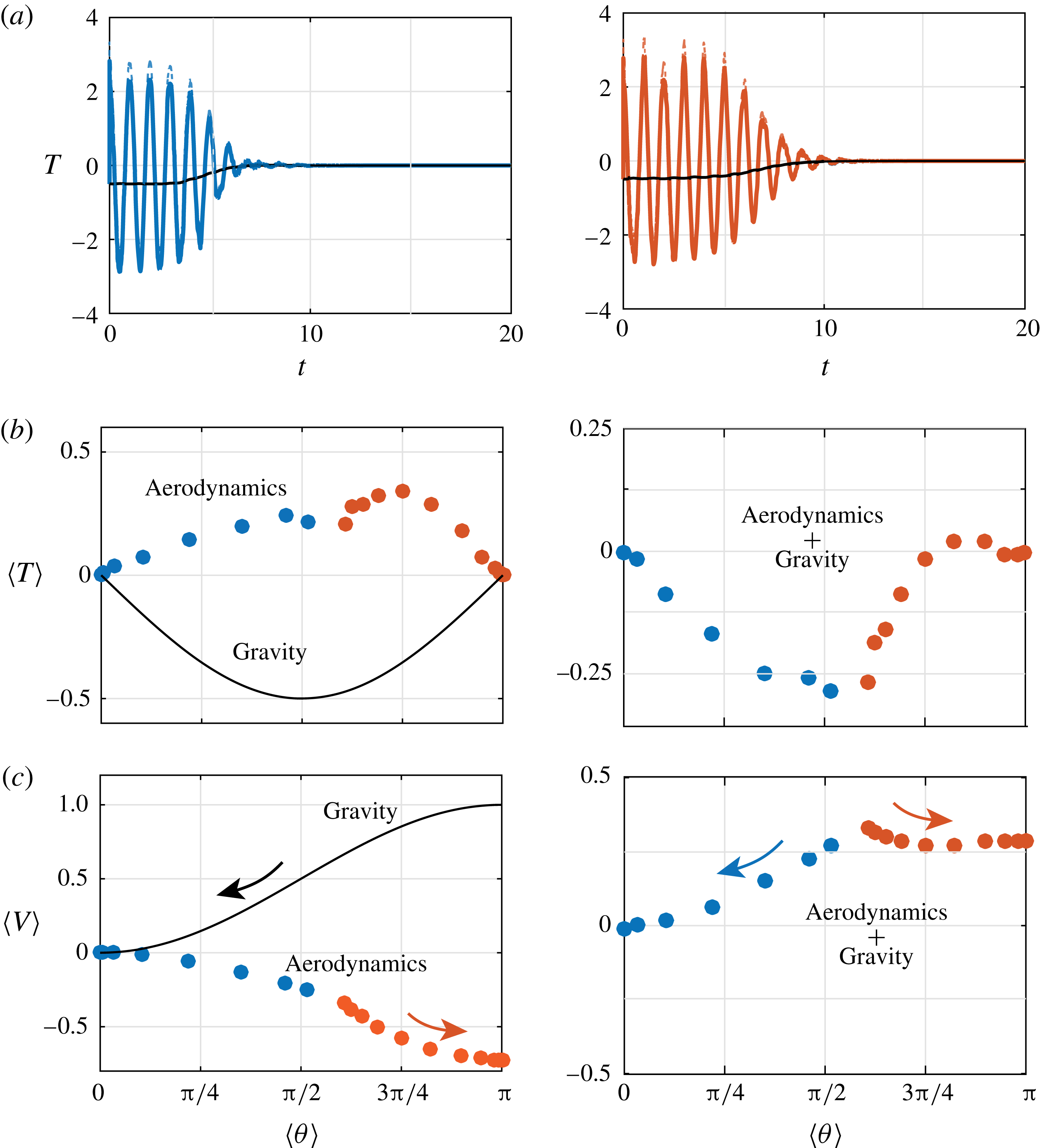
(a) Torque as a function of time for the two trajectories highlighted in figure 5: solid (blue and red) lines denote the total torque which is equal to the aerodynamic torque (dashed lines) and gravitational torque (solid black line). (b,c) Time-averaged torque due to aerodynamics and gravity and corresponding rotational potential
 $V$
as a function of time-averaged orientation.

4.3 Basins of attraction of
 $\wedge$
- and
$\vee$
-configurations


What is the value of the initial perturbation
 $\unicode[STIX]{x1D703}(0)$
beyond which the flyer stabilizes in the concave-up configuration? To answer this question, we vary the initial perturbation
 $\unicode[STIX]{x1D703}(0)$
from
 $0$
to
 $\unicode[STIX]{x03C0}$
by increments
 $\unicode[STIX]{x0394}\unicode[STIX]{x1D703}=\unicode[STIX]{x03C0}/18$
, keeping track of the flyer’s long-term behaviour (concave-down or concave-up). The results are reported in figure 5 for flow parameters
 $\unicode[STIX]{x1D6FD}=0.5$
and
 $\unicode[STIX]{x1D705}=0.5$
and flyers of mass
 $m=1$
and angle
 $\unicode[STIX]{x1D6FC}$
ranging from
 $\unicode[STIX]{x03C0}/18$
to
 $4\unicode[STIX]{x03C0}/9$
. The basin of attraction of the concave-up configuration increases as
 $\unicode[STIX]{x1D6FC}$
increases, allowing for a stable concave-up configuration with perturbations from the upward direction as large as
 $\unicode[STIX]{x03C0}/2$
. Figure 5 also shows the time evolution of
 $\unicode[STIX]{x1D703}(t)$
given two initial conditions
 $\unicode[STIX]{x1D703}(0)=\unicode[STIX]{x03C0}/2$
and
 $\unicode[STIX]{x1D703}(0)=\unicode[STIX]{x03C0}/2+\unicode[STIX]{x03C0}/18$
for a representative example of
 $\unicode[STIX]{x1D6FC}=\unicode[STIX]{x03C0}/3$
. The flyer converges to
 $\unicode[STIX]{x1D703}=0$
in one case and
 $\unicode[STIX]{x1D703}=\unicode[STIX]{x03C0}$
in the other.
For the classic inverted pendulum with
 $\unicode[STIX]{x1D6FD}$
and
 $\unicode[STIX]{x1D705}$
satisfying the condition in (4.2), the limiting value
 $\unicode[STIX]{x1D703}_{o}$
of initial perturbations, averaged over the rapid vertical oscillations, above which the pendulum is stable in the inverted configuration is given by (Butikov Reference Butikov2001, equation (9)),
 $$\begin{eqnarray}\cos (\unicode[STIX]{x1D703}_{o})=-{\displaystyle \frac{1}{2\unicode[STIX]{x03C0}^{2}\unicode[STIX]{x1D6FD}\unicode[STIX]{x1D705}\cos \unicode[STIX]{x1D6FC}}}\left({\displaystyle \frac{2m_{s}}{3(m_{s}-m_{f})}}\right)^{2}.\end{eqnarray}$$
For
 $\unicode[STIX]{x1D705}=\unicode[STIX]{x1D6FD}=0.5$
as in figure 5 and
 $m_{s}/m_{f}=4$
, as
 $\unicode[STIX]{x1D6FC}$
increases from
 $\unicode[STIX]{x03C0}/18$
to
 $4\unicode[STIX]{x03C0}/9$
, the angle
 $\unicode[STIX]{x1D703}_{o}$
marking the boundary of the basin of attraction between the downward stable and upward stable configurations increases from
 $0.55\unicode[STIX]{x03C0}$
to
 $0.87\unicode[STIX]{x03C0}$
. Unlike the flyer, the basin of attraction of the inverted pendulum decreases as
 $\unicode[STIX]{x1D6FC}$
increases.
4.4 Effective rotational potential
To elucidate the fluid mechanical basis of this bistability, we examine the total torques due to both aerodynamics and gravity for the two cases highlighted in figure 5. The torques are shown in figure 6(a) as a function of time. The two subplots are practically indistinguishable because of the fast oscillations in the aerodynamic torque. We therefore average the aerodynamic torque
 $T=T_{1}+T_{2}$
and orientation
 $\unicode[STIX]{x1D703}$
over one period of background flow oscillations to obtain the ‘slow’ quantities,
 $$\begin{eqnarray}\langle T\rangle =\int _{t}^{t+1}T(t^{\prime })\,\text{d}t^{\prime },\quad \langle \unicode[STIX]{x1D703}\rangle =\int _{t}^{t+1}\unicode[STIX]{x1D703}(t^{\prime })\,\text{d}t^{\prime },\end{eqnarray}$$
and we plot
 $\langle T\rangle$
versus
 $\langle \unicode[STIX]{x1D703}\rangle$
in figure 6(b). The slow aerodynamic torque, shown in blue for
 $\unicode[STIX]{x1D703}(0)=\unicode[STIX]{x03C0}/2$
(
 $\wedge$
-stable) and in red for
 $\unicode[STIX]{x1D703}(0)=\unicode[STIX]{x03C0}/2+\unicode[STIX]{x03C0}/18$
(
 $\vee$
-stable), is always positive, indicating that it is acting against gravity in both cases, albeit at slightly higher values in the latter. The torque due to gravity is shown in solid black line and the sum of both torques is shown in the right panel. As
 $\unicode[STIX]{x1D703}\rightarrow \unicode[STIX]{x03C0}$
, the total torque in the
 $\vee$
-stable case becomes positive; the aerodynamic torque overcomes the torque due to gravity.
We define an effective potential function
 $$\begin{eqnarray}V(t)=V(\unicode[STIX]{x1D703}(t))=-\int _{\unicode[STIX]{x1D703}^{\ast }}^{\unicode[STIX]{x1D703}(t)}T(t)\,\text{d}\unicode[STIX]{x1D703}^{\prime }(t),\end{eqnarray}$$
where
 $\unicode[STIX]{x1D703}^{\ast }=0$
for the
 $\wedge$
-stable case and
 $\unicode[STIX]{x1D703}^{\ast }=\unicode[STIX]{x03C0}$
for the
 $\vee$
-stable case. Figure 6(c) shows its slow evolution
 $\langle V\rangle$
, defined according to (4.4), as a function of
 $\langle \unicode[STIX]{x1D703}\rangle$
. The aerodynamic component of this potential counteracts the component due to gravity and dominates as
 $\unicode[STIX]{x1D703}$
approaches
 $\unicode[STIX]{x03C0}$
in the
 $\vee$
-stable case, creating a ‘dip’ in the potential around
 $\unicode[STIX]{x03C0}$
.
It is important to note that the results shown in figure 6(c) do not represent the landscape of the potential function due to aerodynamic and gravitational torques. They rather correspond to a ‘sampling’ of this landscape by two particular trajectories. To construct the aerodynamic potential, we fix the flyer at different angles
 $\unicode[STIX]{x1D703}$
ranging from
 $0$
to
 $\unicode[STIX]{x03C0}$
(no dynamics) and compute the aerodynamic forces and torque at each orientation as detailed in § 4.6. Beforehand, in § 4.5, we provide simple physical arguments to explain the origin and structure of the rotational potential.
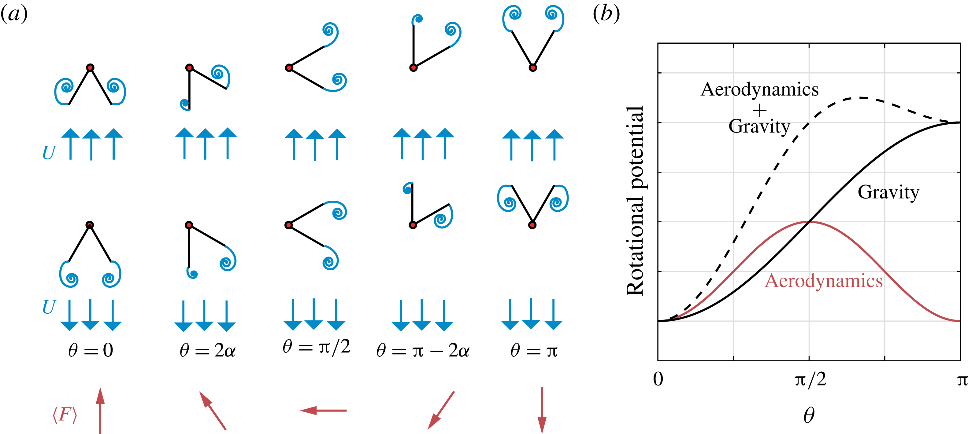
(a) Snapshots of the flyer at various orientations ranging from
 $\unicode[STIX]{x1D703}=0$
to
 $\unicode[STIX]{x1D703}=\unicode[STIX]{x03C0}$
in a uniform flow pointing vertically up (top row) and down (middle row). The direction of the average aerodynamic force over one cycle of flow oscillation is depicted in the bottom row. (b) Schematic of the aerodynamic and gravitational rotational potential.

4.5 Conceptual model
To gain physical insight into the aerodynamic forces acting on the flyer, and the effect of these forces on the aerodynamic torque and rotational potential, we conduct the following thought experiment. The experiment consists of examining a sequence of snapshots of the flyer at various orientations ranging from
 $\unicode[STIX]{x1D703}=0$
to
 $\unicode[STIX]{x1D703}=\unicode[STIX]{x03C0}$
in a uniform flow pointing vertically up or down, as illustrated in figure 7(a). One can immediately make three key observations.
Observation 1: Due to the up–down asymmetry in flyer shape, the wake is not symmetric upon up–down inversion of the uniform flow direction. As a result, the instantaneous aerodynamic force depends on both flyer orientation and flow direction. Consider, for example, the case
 $\unicode[STIX]{x1D703}=0$
(left column of figure 7
a). Since the wake downstream of the flyer is narrower when the flow is pointing down, the resulting aerodynamic drag force is weaker. Under a simplified drag force model, the vertical aerodynamic force
 $F_{y}$
can be expressed in terms of a drag coefficient
 $C_{D}$
that depends on the direction of the uniform flow. Namely, for
 $\unicode[STIX]{x1D703}=0$
, we anticipate
 $F_{y}=C_{D}^{U_{up}}(\unicode[STIX]{x1D70C}_{f}{\mathcal{A}}U^{2}/2)$
when the flow is pointing up and
 $F_{y}=-C_{D}^{U_{down}}(\unicode[STIX]{x1D70C}_{f}{\mathcal{A}}U^{2}/2)$
when the flow is pointing down, with
 $C_{D}^{U_{up}}>C_{D}^{U_{down}}$
. Here,
 ${\mathcal{A}}=2l\cos \unicode[STIX]{x1D6FC}$
is the horizontal projection of the wedge. When averaged over one cycle of flow oscillation, one obtains a net upward force that scales as
 $\langle F_{y}\rangle \sim \unicode[STIX]{x0394}C_{D}(\unicode[STIX]{x1D70C}_{f}{\mathcal{A}}U^{2}/2)$
. Here,
 $\unicode[STIX]{x0394}C_{D}=C_{D}^{Uup}-C_{D}^{Udown}$
reflects the drag asymmetry at
 $\unicode[STIX]{x1D703}=0$
, which depends on the flyer opening angle,
 $\unicode[STIX]{x1D6FC}$
. Note that the scaling presented above is consistent with the quasi-steady drag model proposed in Weathers et al. (Reference Weathers, Folie, Liu, Childress and Zhang2010).
Observation 2: By comparing the first and last column in figure 7(a), it is evident that up–down inversion of the wedge does not change the magnitude of the net vertical force
 $\langle F_{y}\rangle$
, only its direction. In other words,
 $\langle F_{y}\rangle |_{\unicode[STIX]{x1D703}=\unicode[STIX]{x03C0}}=-\langle F_{y}\rangle |_{\unicode[STIX]{x1D703}=0}$
. Further, at
 $\unicode[STIX]{x1D703}=\unicode[STIX]{x03C0}/2$
, we anticipate no net vertical force,
 $\langle F_{y}\rangle =0$
, due to the up–down symmetry in flyer shape at this orientation (see middle column in figure 7
a). Based on the flow- and orientation dependence described in observations 1 and 2, we anticipate that
 $\langle F_{y}\rangle \sim \unicode[STIX]{x0394}C_{D}\cos \unicode[STIX]{x1D703}$
.
Observation 3: The horizontal component of the force ought to be zero at
 $\unicode[STIX]{x1D703}=0$
and
 $\unicode[STIX]{x1D703}=\unicode[STIX]{x03C0}$
due to the left–right symmetry of the flyer and negative at
 $\unicode[STIX]{x1D703}=\unicode[STIX]{x03C0}/2$
due to the net circulation in the wake. This observation suggests
 $\langle F_{x}\rangle \sim -C_{L}\sin (\unicode[STIX]{x1D703})$
, where
 $C_{L}$
is the lift coefficient at
 $\unicode[STIX]{x1D703}=\unicode[STIX]{x03C0}/2$
, which depends on
 $\unicode[STIX]{x1D6FC}$
.
Put together, these three observations imply that, over one cycle of flow oscillation, the net horizontal force is symmetric and the vertical force is anti-symmetric about
 $\unicode[STIX]{x1D703}=\unicode[STIX]{x03C0}/2$
, i.e. for an up–down reflection of the wedge. These symmetries exist for all angles
 $\unicode[STIX]{x1D6FC}$
and can be easily traced back to the left–right symmetry of the flyer and up–down symmetry of the oscillating background flow. In addition, given these scaling laws for
 $\langle F_{y}\rangle$
and
 $\langle F_{x}\rangle$
, one can posit that the net rotational torque acting on the wedge varies with
 $\unicode[STIX]{x1D6FC}$
and
 $\unicode[STIX]{x1D703}$
as
 $$\begin{eqnarray}\langle T\rangle \sim \langle F_{y}\rangle \sin \unicode[STIX]{x1D703}+\langle F_{x}\rangle \cos \unicode[STIX]{x1D703}\sim (\unicode[STIX]{x0394}C_{D}-C_{L})\sin (2\unicode[STIX]{x1D703}).\end{eqnarray}$$
Hence, the rotational potential associated with the aerodynamic torque scales as
 $$\begin{eqnarray}\langle V\rangle =-\int _{0}^{\unicode[STIX]{x1D703}}\langle T\rangle \,\text{d}\unicode[STIX]{x1D703}^{\prime }\sim {\displaystyle \frac{1}{2}}(\unicode[STIX]{x0394}C_{D}-C_{L})[\cos (2\unicode[STIX]{x1D703})-1].\end{eqnarray}$$
An important consequence of this analysis is that the rotational potential due to aerodynamics is symmetric about
 $\unicode[STIX]{x1D703}=\unicode[STIX]{x03C0}/2$
. The up–down asymmetry in flyer shape, and therefore, vertical force, does not translate into an asymmetry in the rotational torque in favour of one configuration (concave-up
 $\vee$
) versus another (concave-down
 $\wedge$
). From an aerodynamic perspective, both configurations are rotationally equivalent in an oscillating flow, as illustrated by the aerodynamic potential in figure 7(b). This new insight completes the picture presented in figure 1(c) of Liu et al. (Reference Liu, Ristroph, Weathers, Childress and Zhang2012), which focused solely on the local stability of the hovering pyramid around
 $\unicode[STIX]{x1D703}=0$
.
Importantly, the asymmetry in the gravitational potential breaks the symmetry in the aerodynamic potential (see figure 7
b). If the aerodynamic potential well at
 $\unicode[STIX]{x1D703}=\unicode[STIX]{x03C0}$
is deep enough, the resulting total potential can have a dip at
 $\unicode[STIX]{x1D703}=\unicode[STIX]{x03C0}$
that stabilizes the concave-up
 $\vee$
configuration. In the next section, we verify these conceptual predictions using the vortex sheet model. We also derive quantitative expressions for the aerodynamic forces, torque and rotational potential averaged over one period of fast oscillations. Keep in mind that the discussion above, and the presence of a well in the aerodynamic potential at
 $\unicode[STIX]{x1D703}=0$
and
 $\unicode[STIX]{x1D703}=\unicode[STIX]{x03C0}$
, requires that
 $C_{L}>\unicode[STIX]{x0394}C_{D}$
. If the drag asymmetry is dominant,
 $\unicode[STIX]{x0394}C_{D}>C_{L}$
, the aerodynamic potential would have a well at
 $\unicode[STIX]{x1D703}=\unicode[STIX]{x03C0}/2$
, i.e. aerodynamic forces would serve to stabilize the flyer in the up–down symmetric orientation corresponding to
 $\unicode[STIX]{x1D703}=\unicode[STIX]{x03C0}/2$
.
4.6 Aerodynamic forces and torques and slow rotational potential
In this section, we construct the landscape of the rotational potential by averaging the unsteady aerodynamics over fast oscillations of the background flow. We begin by fixing the flyer at different angles
 $\unicode[STIX]{x1D703}$
ranging from
 $0$
to
 $\unicode[STIX]{x03C0}$
in a fluid oscillating with amplitude
 $\unicode[STIX]{x1D6FD}=0.5$
and acceleration
 $\unicode[STIX]{x1D705}=0.5$
. At each orientation
 $\unicode[STIX]{x1D703}$
, we compute the aerodynamic forces
 $\langle F_{x}\rangle$
and
 $\langle F_{y}\rangle$
based on the vortex sheet model (see (3.3)) and averaged over fast flow oscillations. Results are shown in figure 8(a,b) for three flyers of half-opening angle
 $\unicode[STIX]{x1D6FC}=\unicode[STIX]{x03C0}/6,\unicode[STIX]{x03C0}/4$
and
 $\unicode[STIX]{x03C0}/3$
. Given the left–right symmetry of the flyer and the up–down symmetry of flow oscillations,
 $\langle F_{x}\rangle$
is symmetric about the horizontal axis
 $\unicode[STIX]{x1D703}=\unicode[STIX]{x03C0}/2$
while
 $\langle F_{y}\rangle$
is anti-symmetric. Importantly, for
 $\unicode[STIX]{x1D703}<\unicode[STIX]{x03C0}/2$
,
 $\langle F_{y}\rangle$
points in the opposite direction to gravity whereas for
 $\unicode[STIX]{x1D703}>\unicode[STIX]{x03C0}/2$
,
 $\langle F_{y}\rangle$
reinforces gravity. We emphasize that we do not impose these symmetries a priori; they arise naturally in the vortex sheet simulations. These symmetries are also consistent with physical intuition, as discussed in § 4.5.
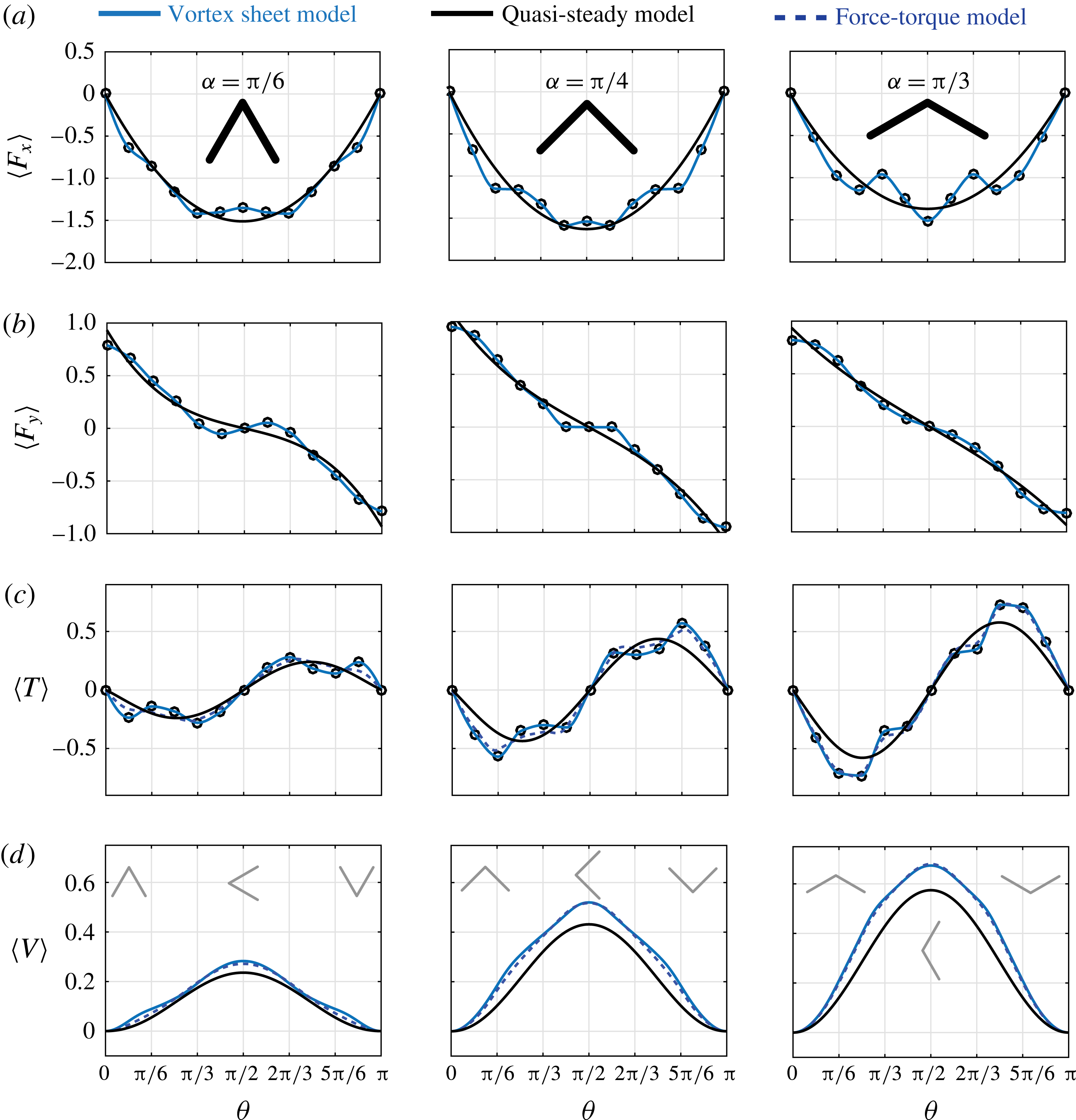
(a–c) Aerodynamic forces
 $\langle F_{x}\rangle$
,
 $\langle F_{y}\rangle$
, torque
 $\langle T\rangle$
averaged over one oscillation period as a function of
 $\unicode[STIX]{x1D703}$
based on the vortex sheet model (solid blue line) and the quasi-steady point-force model (solid black line). (d) Effective rotational potential
 $V$
as a function of
 $\unicode[STIX]{x1D703}$
. Nominal parameter values are set to
 $m=1$
and
 $\unicode[STIX]{x1D705}=\unicode[STIX]{x1D6FD}=0.5$
.

We postulate a slow point-force model that takes into account these symmetries as follows
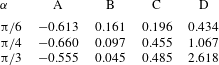
 $$\begin{eqnarray}\langle F_{x}\rangle =A\unicode[STIX]{x1D703}(\unicode[STIX]{x03C0}-\unicode[STIX]{x1D703}),\quad \langle F_{y}\rangle =B\left({\displaystyle \frac{\unicode[STIX]{x03C0}}{2}}-\unicode[STIX]{x1D703}\right)^{3}+C\left({\displaystyle \frac{\unicode[STIX]{x03C0}}{2}}-\unicode[STIX]{x1D703}\right).\end{eqnarray}$$
Here, the constant parameters
 $A$
,
 $B$
and
 $C$
depend on the flyer’s angle
 $\unicode[STIX]{x1D6FC}$
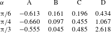
. The values obtained from a least-square fit between the point-force model and the forces computed based on the vortex sheet model are listed in table 3. The expressions in (4.8) can be viewed as Taylor series expansions about
 $\unicode[STIX]{x1D703}=\unicode[STIX]{x03C0}/2$
of the sine and cosine functions proposed in § 4.5, noting that
 $\sin (\unicode[STIX]{x03C0}/2-\unicode[STIX]{x1D703})=\cos \unicode[STIX]{x1D703}$
and
 $\cos (\unicode[STIX]{x03C0}/2-\unicode[STIX]{x1D703})=\sin \unicode[STIX]{x1D703}$
. The ‘quasi-steady’ point-force model is superimposed on figure 8(a,b), showing good agreement with the vortex sheet model for all flyers.
We compute the aerodynamic torque about the flyer’s point of attachment using (3.3) and take its time average
 $\langle T\rangle$
over the fast flow oscillations as in (4.4); see figure 8(c). The torque is anti-symmetric about the horizontal axis
 $\unicode[STIX]{x1D703}=\unicode[STIX]{x03C0}/2$
: it is negative for
 $\unicode[STIX]{x1D703}<\unicode[STIX]{x03C0}/2$
(reinforcing gravity) and positive for
 $\unicode[STIX]{x03C0}/2<\unicode[STIX]{x1D703}<\unicode[STIX]{x03C0}$
. At first glance, this seems inconsistent with figure 6(c) where the aerodynamic torques act against gravity for all
 $\langle \unicode[STIX]{x1D703}\rangle$
averaged over fast flow oscillations. However, this discrepancy arises because the plots in figure 6(c) correspond to time-averaged values obtained from dynamic trajectories where the rotational momentum varies in time. In figure 8, the flyer is held fixed in order to extract the inherent symmetries in the aerodynamic forces and torque induced by the oscillatory flow itself. Further, note that this analysis is consistent with the point-force model presented in Liu et al. (Reference Liu, Ristroph, Weathers, Childress and Zhang2012, figure 3) for the particular case
 $\unicode[STIX]{x1D6FC}=\unicode[STIX]{x03C0}/6$
. In Liu et al. (Reference Liu, Ristroph, Weathers, Childress and Zhang2012), the aerodynamic forces were postulated to act at the outer two edges of the flyer (at the sites of vortex emission) and their directions and magnitudes were assumed to follow ad hoc rules motivated by symmetry arguments. Based on these rules, the aerodynamic torque was computed about the flyer’s centre of mass. Here, the aerodynamic forces and torque are computed exactly based on the vortex sheet model and the point-force model is built accordingly with no further assumptions. As such, our force model incorporates the unsteady aerodynamics and is applicable to flyers of any shape
 $\unicode[STIX]{x1D6FC}$
.
Equations (3.3) do not reflect the location of the aerodynamic centre where the aerodynamic forces should be applied in order to produce an equivalent aerodynamic torque. To this end, we postulate that the force should act along the axis of symmetry of the flyer for all
 $\unicode[STIX]{x1D703}$
and we write
 $$\begin{eqnarray}\langle T\rangle =Dl\cos \unicode[STIX]{x1D6FC}(\langle F_{x}\rangle \cos \unicode[STIX]{x1D703}+\langle F_{y}\rangle \sin \unicode[STIX]{x1D703}),\end{eqnarray}$$
where
 $D$
is an unknown parameter that reflects the distance from the flyer’s apex to the aerodynamic centre. The values of
 $D$
listed in the last column of table 3 are obtained from a least-square fit between the values of
 $\langle T\rangle$
computed directly from (3.3) and those calculated from (4.9) with forces computed from (3.3). For
 $\unicode[STIX]{x1D6FC}=\unicode[STIX]{x03C0}/6$
, the aerodynamic centre is close to the centre of mass of the flyer (
 $D\approx 0.5$
) as postulated in Liu et al. (Reference Liu, Ristroph, Weathers, Childress and Zhang2012). However, as
 $\unicode[STIX]{x1D6FC}$
increases,
 $D$
also increases. For
 $\unicode[STIX]{x1D6FC}=\unicode[STIX]{x03C0}/3$
,
 $D$
is larger than five times the distance between the apex and the centre of mass.
Lastly, we compute the rotational potential
 $\langle V\rangle$
due to aerodynamics such that
 $\langle T\rangle =-\unicode[STIX]{x2202}\langle V\rangle /\unicode[STIX]{x2202}\unicode[STIX]{x1D703}$
. Figure 8(d) shows three lines: the solid blue line is based on the vortex sheet model; the dashed blue line is based on the force-torque model in (4.9) with forces obtained from the vortex sheet model; the solid black line is based on (4.9) and the quasi-steady model in (4.8). The difference between the quasi-steady and vortex sheet models increases as the angle
 $\unicode[STIX]{x1D6FC}$
of the flyer increases. For all
 $\unicode[STIX]{x1D6FC}$
, the aerodynamic potential is symmetric about
 $\unicode[STIX]{x03C0}/2$
and is characterized by two minima at
 $\unicode[STIX]{x1D703}=0$
and
 $\unicode[STIX]{x1D703}=\unicode[STIX]{x03C0}$
. The potential wells around these minima are indistinguishable. This symmetry is broken in the presence of gravity. When the rotational potential
 $(m\unicode[STIX]{x1D6FD}/\unicode[STIX]{x1D705})\cos \unicode[STIX]{x1D6FC}\cos \unicode[STIX]{x1D703}$
due to gravity is added, the well around
 $\unicode[STIX]{x1D703}=\unicode[STIX]{x03C0}$
becomes more shallow and disappears altogether when gravity is dominant.
In summary, for
 $\unicode[STIX]{x1D703}<\unicode[STIX]{x03C0}/2$
, as
 $\unicode[STIX]{x1D6FC}$
increases from
 $\unicode[STIX]{x1D6FC}=\unicode[STIX]{x03C0}/6$
to
 $\unicode[STIX]{x03C0}/3$
, the
 $\wedge$
-configuration gets more stable. At the same time, the aerodynamic centre gets pushed below the centre of mass. Taken together, these two observations are consistent with the experimental findings in Liu et al. (Reference Liu, Ristroph, Weathers, Childress and Zhang2012) that top-heavy flyers are more stable. Meanwhile, For
 $\unicode[STIX]{x1D703}>\unicode[STIX]{x03C0}/2$
, the same is true about the
 $\vee$
-configuration. However, force calculations show that only the
 $\wedge$
-configuration and perturbations smaller than
 $\unicode[STIX]{x03C0}/2$
produce aerodynamic forces that can potentially sustain the flyer’s mass when released from the attachment point, as in Weathers et al. (Reference Weathers, Folie, Liu, Childress and Zhang2010), Liu et al. (Reference Liu, Ristroph, Weathers, Childress and Zhang2012), Huang et al. (Reference Huang, Nitsche and Kanso2015, Reference Huang, Nitsche and Kanso2016).
The quasi-steady model presented here can be used as a predictive tool in problems involving
 $\wedge$
-shaped bodies in oscillatory flows. To this end, one would have to start from the equations of motion, such as those in (2.4), and rewrite all variables in terms of ‘fast’ and ‘slow’ components to arrive at two sets of equations describing the fast and slow dynamics of the system. The slow component of the aerodynamic torque can be read directly from figure 8 or from (4.8), (4.9) and table 3. This undertaking is beyond the scope of the present paper and will be addressed in a future study.
5 Results: elastic flyers
To examine the effect of flexibility on the flyer’s response, we introduce a rotational spring at the apex between the two wings for a flyer of mass
 $m=1$
. We fix the rest angle of the spring at
 $\unicode[STIX]{x1D6FC}_{r}=\unicode[STIX]{x03C0}/6$
and consider four values of the stiffness coefficient:
 $k_{e}=1000,100,50$
and
 $10$
. Smaller stiffness implies more compliant flyer. For infinitely large
 $k_{e}$
, we recover the rigid flyer whose parameter space
 $(\unicode[STIX]{x1D6FD},\unicode[STIX]{x1D705})$
is depicted in the middle panel of figure 4(b). Here, we map the behaviour of the elastic flyer onto the same parameter space
 $(\unicode[STIX]{x1D6FD},\unicode[STIX]{x1D705})$
for each value of
 $k_{e}$
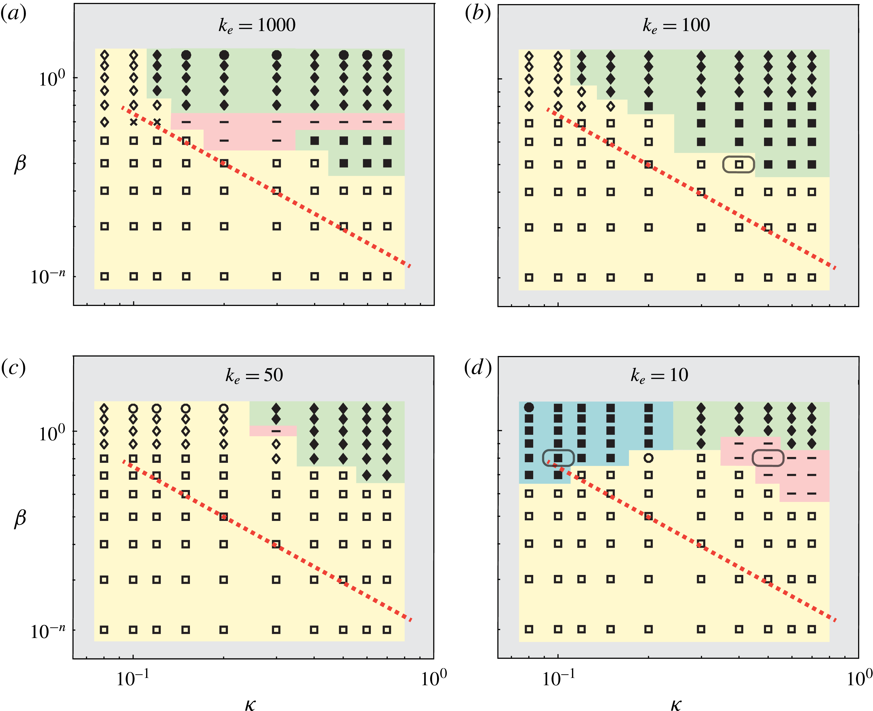
; see figure 9. Similar to its rigid analogue, the elastic flyer exhibits stable and bistable behaviour but the transition to bistable behaviour is pushed up and to the right in the
 $(\unicode[STIX]{x1D705},\unicode[STIX]{x1D6FD})$
plane. In other words, the bistable region is smaller for
 $k_{e}=1000$
. The red line in figure 4(b) (middle panel) marking the transition of the rigid flyer to bistability is overlaid onto the parameter space of the elastic flyer for ease of comparison.
Stable and bistable behaviour of an elastic flyer mapped onto the (
 $\unicode[STIX]{x1D705}$
,
 $\unicode[STIX]{x1D6FD}$
) space for decreasing spring stiffness
 $k_{e}=1000,100,50,10$
. The mass and rest angle are set to
 $m=1$
and
 $\unicode[STIX]{x1D6FC}_{r}=\unicode[STIX]{x03C0}/6$
as in the middle panel of figure 4(b). The open symbols ‘▫’ ‘♢’ and ‘○’ correspond to stable concave-down
 $\wedge$
-configuration, with ‘▫’ representing asymptotically stable behaviour (
 $\unicode[STIX]{x1D703}\rightarrow 0$
) and ‘♢’ and ‘○’ representing bounded chaotic-like and periodic oscillations about
 $\unicode[STIX]{x1D703}=0$
, respectively. The filled symbols ‘▪’ ‘♦’ and ‘●’ are used to denote bistable behaviour. The symbol ‘–’ represents a new behaviour where the elastic flyer is stable about an inclined orientation not equal to
 $\unicode[STIX]{x03C0}$
. For comparison, the dashed lines from figure 4 marking the transition to bistable behaviour of the rigid flyer are overlaid.

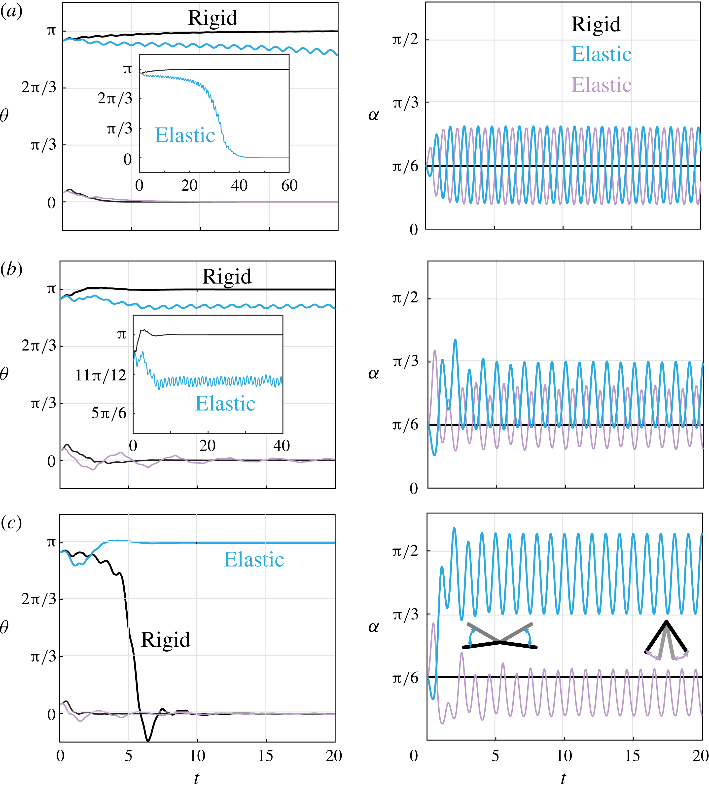
Elastic versus rigid flyers of mass
 $m=1$
and (rest) angle
 $\unicode[STIX]{x1D6FC}_{r}=\unicode[STIX]{x03C0}/6$
for three sets of parameters highlighted in grey boxes in figure 9. (a)
 $\unicode[STIX]{x1D705}=0.4$
,
 $\unicode[STIX]{x1D6FD}=0.5$
,
 $k_{e}=100$
, (b)
 $\unicode[STIX]{x1D705}=0.5$
,
 $\unicode[STIX]{x1D6FD}=0.8$
,
 $k_{e}=10$
and (c)
 $\unicode[STIX]{x1D705}=0.1$
,
 $\unicode[STIX]{x1D6FD}=0.8$
,
 $k_{e}=10$
. Initial conditions are
 $\unicode[STIX]{x1D703}(0)=\unicode[STIX]{x03C0}/18$
and
 $17\unicode[STIX]{x03C0}/18$
,
 $\dot{\unicode[STIX]{x1D703}}(0)=0$
and
 $\unicode[STIX]{x1D6FC}(0)-\unicode[STIX]{x1D6FC}_{r}=\dot{\unicode[STIX]{x1D6FC}}(0)=0$
.

A new behaviour is observed in flexible flyers at
 $k_{e}=1000$
. The new behaviour is marked by ‘
 $-$
’ and highlighted in pink. It is characterized by the flyer being stable about an inclined orientation not equal to
 $\unicode[STIX]{x03C0}$
. For
 $k_{e}=100$
, the new behaviour disappears and the bistable region increases slightly relative to that at
 $k_{e}=1000$
but remains smaller than that of the rigid flyer. As
 $k_{e}$
decreases to
 $50$
, the new behaviour reappears and the bistable region shrinks again, indicating that the size of the bistable region varies non-monotonically with
 $k_{e}$
. In fact, it seems that
 $k_{e}=100$
is optimal for maximizing the bistable region above the red line. Finally, for
 $k_{e}=10$
, the bistable behaviour about inclined orientations reappears in the upper right region of
 $(\unicode[STIX]{x1D6FD},\unicode[STIX]{x1D705})$
space. Importantly, bistable behaviour appears in the upper left corner at high values of
 $\unicode[STIX]{x1D6FD}$
and low values of
 $\unicode[STIX]{x1D705}$
(region highlighted in blue). This new transition to bistability seems unique to highly flexible flyers, and may be associated with the limit where gravitational and elastic forces are comparable, that is to say,
 $O(m\unicode[STIX]{x1D6FD}/\unicode[STIX]{x1D705})\sim O(k_{e})$
in (2.4).
To shed more light on the difference in behaviour between the flexible flyer and its rigid analogue, we show in figure 10 the time evolution of
 $\unicode[STIX]{x1D703}$
and
 $\unicode[STIX]{x1D6FC}$
for three representative cases highlighted in grey boxes in figure 9(b,d). Figure 10(a) shows the flyer’s orientation
 $\unicode[STIX]{x1D703}$
and flapping angle
 $\unicode[STIX]{x1D6FC}$
about the rest angle
 $\unicode[STIX]{x1D6FC}_{r}=\unicode[STIX]{x03C0}/6$
of the spring as functions of time for
 $\unicode[STIX]{x1D705}=0.4$
,
 $\unicode[STIX]{x1D6FD}=0.5$
and
 $k_{e}=100$
. Here, elasticity destabilizes the upward configuration.
Figure 10(b) shows the new behaviour highlighted in pink in figure 9. The parameter values are set to
 $\unicode[STIX]{x1D705}=0.5$
,
 $\unicode[STIX]{x1D6FD}=0.8$
and
 $k_{e}=10$
. The flyer stabilizes about an upward configuration around
 $\unicode[STIX]{x1D703}=11\unicode[STIX]{x03C0}/12$
rather than
 $\unicode[STIX]{x03C0}$
. The associated shape oscillations occur about a larger opening angle than the spring’s rest angle.
Finally, figure 10(c) shows the new transition to bistable behaviour at
 $\unicode[STIX]{x1D705}=0.1$
,
 $\unicode[STIX]{x1D6FD}=0.8$
and
 $k_{e}=10$
. The right panel of figure 10(c) shows the flyer’s flapping behaviour. The inset schematics depict the range of flapping angles for the upward and downward stable trajectories. Because the flyer is compliant, it flaps about a much larger angle than the spring rest angle, thus increasing the effective opening angle of the flyer and the resulting aerodynamic torque. The flyer can therefore stabilize upward at much lower values of flow acceleration. However, in this flexible limit, the distinction between concave-up and concave-down is not very clear because the flyer exhibits both types of concavity over one oscillation cycle.
In all three examples, the frequency of the flapping motion is equal to the frequency of the background flow, irrespective of initial conditions and parameter values. That is to say, the frequency of flapping
 $\unicode[STIX]{x1D6FC}$
is slaved to aerodynamics rather than to the intrinsic natural frequency associated with the flyer’s elasticity. We calculate the intrinsic natural frequency of the flyer as follows. We linearize (2.4), with aerodynamic torques set to zero, about the equilibrium configuration
 $(0,\unicode[STIX]{x1D6FC}^{\ast })$
of the ‘dry’ system. To this end,
 $\unicode[STIX]{x1D6FC}^{\ast }$
is given by
 $$\begin{eqnarray}\sin \unicode[STIX]{x1D6FC}^{\ast }=\frac{k_{e}\unicode[STIX]{x1D705}}{m\unicode[STIX]{x1D6FD}}(\unicode[STIX]{x1D6FC}_{r}-\unicode[STIX]{x1D6FC}^{\ast }),\end{eqnarray}$$
and
 $\unicode[STIX]{x1D6FC}_{r}-m\unicode[STIX]{x1D6FD}/k_{e}\unicode[STIX]{x1D705}\leqslant \unicode[STIX]{x1D6FC}^{\ast }\leqslant \unicode[STIX]{x1D6FC}_{r}$
. The linear equations are
 $$\begin{eqnarray}\unicode[STIX]{x1D6FF}\ddot{\unicode[STIX]{x1D703}}+\left(\frac{\unicode[STIX]{x1D6FD}}{\unicode[STIX]{x1D705}}\cos \unicode[STIX]{x1D6FC}^{\ast }\right)\unicode[STIX]{x1D6FF}\unicode[STIX]{x1D703}=0,\quad \unicode[STIX]{x1D6FF}\ddot{\unicode[STIX]{x1D6FC}}+\left(\frac{k_{e}}{m}+\frac{\unicode[STIX]{x1D6FD}}{\unicode[STIX]{x1D705}}\cos \unicode[STIX]{x1D6FC}^{\ast }\right)\unicode[STIX]{x1D6FF}\unicode[STIX]{x1D6FC}=0.\end{eqnarray}$$
The first equation leads to the rotational natural frequency of the classic pendulum. The natural frequency
 $f_{n}^{\unicode[STIX]{x1D6FC}}$
of shape oscillations follows from the second equation,
 $$\begin{eqnarray}f_{n}^{\unicode[STIX]{x1D6FC}}=\frac{1}{2\unicode[STIX]{x03C0}}\sqrt{\frac{k_{e}}{m}+\frac{\unicode[STIX]{x1D6FD}}{\unicode[STIX]{x1D705}}\cos \unicode[STIX]{x1D6FC}^{\ast }}.\end{eqnarray}$$
For
 $k_{e}=10$
, the natural frequency
 $f_{n}^{\unicode[STIX]{x1D6FC}}$
is about
 $1/2$
.
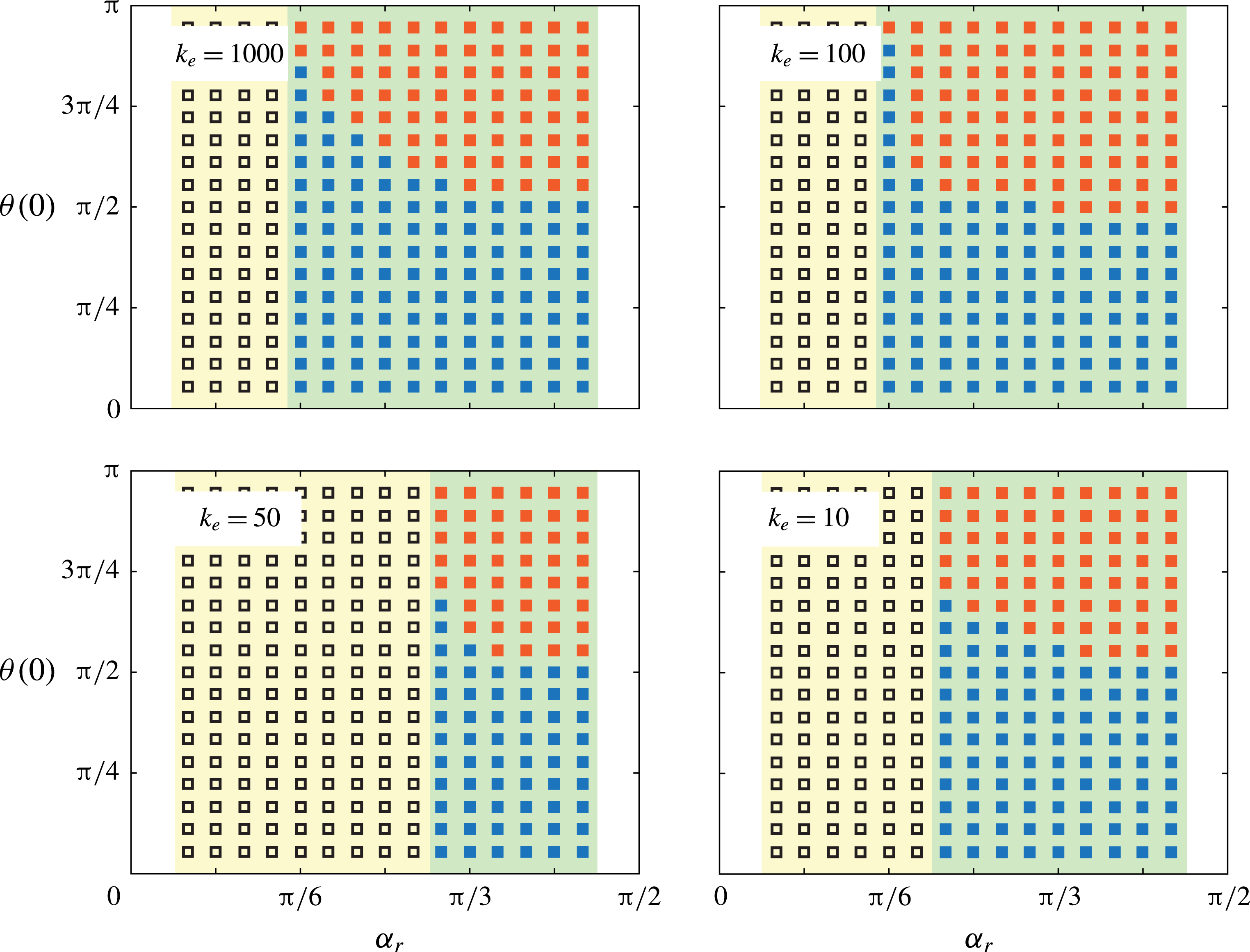
Basins of attraction for the (blue) downward
 $\wedge$
- and (red) upward
 $\vee$
-stable configurations vary with the spring stiffness
 $k_{e}=1000,100,50,10$
and the spring’s rest angle
 $\unicode[STIX]{x1D6FC}_{r}$
. Parameters are set to
 $\unicode[STIX]{x1D6FD}=0.5$
and
 $\unicode[STIX]{x1D705}=0.5$
and
 $m=1$
. The open symbols ‘▫’ correspond to stable concave-down
 $\wedge$
-configuration while the filled symbols ‘▪’ denote bistable behaviour.

Lastly, we examine the effect of elasticity on the ‘basin of attraction’ of the vertically upward configuration. Figure 11 shows that, in comparison with the rigid flyer in figure 5, the introduction of a stiff spring
 $k_{e}=1000$
has a small effect on the basin of attraction of
 $\unicode[STIX]{x1D703}=\unicode[STIX]{x03C0}$
. As
 $k_{e}$
decreases, this basin seems to increase and it is maximum at
 $k_{e}=100$
. As
 $k_{e}$
decreases further (
 $k_{e}=50$
), the region of bistable behaviour decreases but not the basin of attraction. Finally, for
 $k_{e}=10$
, both the region of bistable behaviour and the basin of attraction of
 $\unicode[STIX]{x1D703}=\unicode[STIX]{x03C0}$
increase, certainly due to an increase in the effective opening angle of the compliant flyer.
6 Conclusions
The main contributions of this work can be summarized as follows. We considered the rotational stability of a
 $\wedge$
-flyer of half-opening angle
 $\unicode[STIX]{x1D6FC}$
attached at its apex and free to rotate in a vertically oscillating flow. We found that aerodynamic effects stabilize the upward
 $\vee$
-configuration for a range of background flow parameters, namely, amplitude and frequency of oscillations. We compared these parameters to those required to stabilize a ‘dry’ pendulum in the upward configuration via fast vertical oscillations of its base, i.e. the classical inverted pendulum. We found that aerodynamics can induce upward stability at lower oscillation frequency and amplitude. Importantly, the upward configuration can be stable even under perturbations as large as
 $\unicode[STIX]{x03C0}/2$
. We explained the aerodynamic origin of this bistability about the downward and upward configurations by analysing in detail the aerodynamic forces and torques acting on the flyer. To this end, we employed the vortex sheet model and we averaged over the fast oscillations of the background flow in order to develop a slow rotational potential that takes into account the geometry of the flyer as well as the unsteady aerodynamics. Lastly, we introduced an elastic spring at the apex of the flyer and allowed it to flap passively under background flow oscillations. We found that the flapping frequency always corresponds to the frequency of the background flow. For the parameter ranges considered here, the intrinsic frequency of the flyer does not play a role. Elasticity diminishes upward stability in stiff flyers. However, with further decrease in stiffness, we observed a new transition to upward stability. This transition is induced by large-amplitude flapping motion of the flyer.
Our force calculations show that due to up–down asymmetry,
 $\wedge$
-flyers can use aerodynamic forces to support their weight only when the perturbation from the concave-down
 $\wedge$
-configuration is less than
 $\unicode[STIX]{x03C0}/2$
, in agreement with Weathers et al. (Reference Weathers, Folie, Liu, Childress and Zhang2010), Liu et al. (Reference Liu, Ristroph, Weathers, Childress and Zhang2012), Huang et al. (Reference Huang, Nitsche and Kanso2015, Reference Huang, Nitsche and Kanso2016). Further, our results suggest that stable
 $\wedge$
-configurations can be maintained by manipulating either the opening angle or stiffness of the flyer. These findings will guide the development of future research aimed at understanding the rotational stability of biological and bio-inspired flyers. Insects use flight muscles attached at the base of the wings to flap (Pringle Reference Pringle2003). Insect wings and flight muscles are thought to be stiff (Ellington Reference Ellington1985) but organisms can modulate their muscle stiffness (Feldman & Levin Reference Feldman and Levin2009). It is therefore plausible that, by manipulating the stiffness of their flight muscle, insects can maintain stability in the face of environmental disturbances. The idealized model presented in this paper overly simplifies the wing–muscle system in insects, which includes both active and passive components. However, the model and results presented here can be used as a first step towards developing a more accurate wing–muscle model and to incorporate feedback control, allowing the muscle stiffness to adaptively change in response to flow perturbations. Another future direction will be to examine the effects of the opening angle on the stability of both gliding and flapping flight. In the latter, we allow the flyer to oscillate in an otherwise quiescent fluid. Our preliminary results suggest that for a flapping flyer, inertial effects akin to those present in the inverted pendulum play a role in stabilizing the flyer. These findings will be reported in future work.
Acknowledgements
The work of Y.H. and E.K. is supported by the National Science Foundation (NSF) through the grants NSF CMMI 13-63404 and NSF CBET 15-12192 and by the Army Research Office (ARO) through the grant W911NF-16-1-0074. E.K. would like to thank Mr S. Heydari for assistance in analysing the effect of dissipation time on the aerodynamic force.
Appendix. Aerodynamic force as a function of dissipation time
In order to assess the effect of the dissipation time
 $\unicode[STIX]{x1D70F}_{diss}$
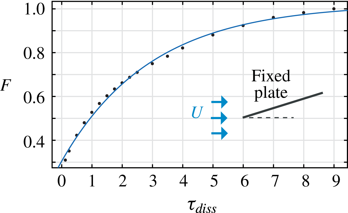
on the aerodynamic forces acting on the flyer, we consider a slightly simpler problem of a flat plate fixed at one end in an oncoming uniform flow. Figure 12 shows the magnitude
 $F$
of the total aerodynamic force as a function of
 $\unicode[STIX]{x1D70F}_{diss}$
for a plate held at a fixed angle of attack
 $\unicode[STIX]{x03C0}/12$
. For a given value of
 $\unicode[STIX]{x1D70F}_{diss}$
, there is an effective ‘dissipation’ force that is equal to the difference between the value of
 $F$
as
 $\unicode[STIX]{x1D70F}_{diss}\rightarrow \infty$
and the value of
 $F$
at
 $\unicode[STIX]{x1D70F}_{diss}$
. While
 $F$
increases as
 $\unicode[STIX]{x1D70F}_{diss}$
increases, the dissipation force decreases, in agreement with physical intuition.
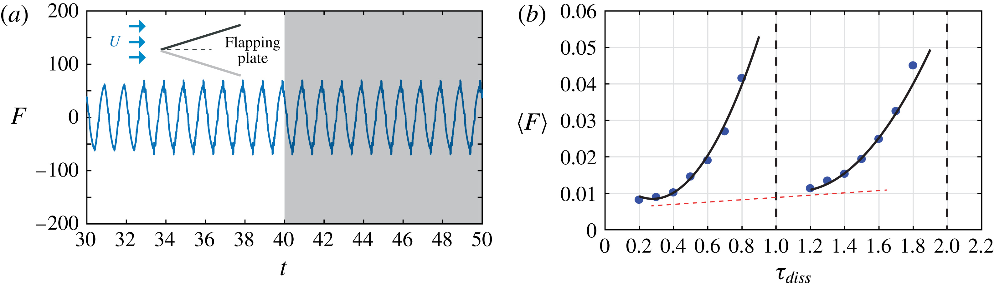
In figure 13, we consider the aerodynamic force acting on a plate undergoing pitching oscillations in uniform flow. The wake structure and force acting on a pitching plate were computed in Sheng et al. (Reference Sheng, Ysasi, Kolomenskiy, Kanso, Nitsche, Schneider, Childress, Hosoi, Schultz and Wang2012) using three different models: a high-fidelity Navier–Stokes simulation, a vortex sheet model, and an unsteady point vortex model. The three models showed good agreement in the wake structure but some deviation in the force value. Here, we restrict ourselves to the vortex sheet model. Figure 13(a) shows the force magnitude versus time for oscillation amplitude
 $\unicode[STIX]{x03C0}/12$
, frequency
 $1$
and
 $\unicode[STIX]{x1D70F}_{diss}=1.5$
. The total integration time is equivalent to fifty cycles of oscillations. Figure 13(b) shows the force magnitude averaged over the last ten oscillation cycles versus
 $\unicode[STIX]{x1D70F}_{diss}$
. The force behaviour is more complicated than that of the fixed plate: the force increases as
 $\unicode[STIX]{x1D70F}_{diss}\rightarrow nT$
, where
 $T=1$
is the period of oscillation of the plate and
 $n$
is an integer. The reason is that at
 $\unicode[STIX]{x1D70F}_{diss}=nT$
, the force induced by
 $\unicode[STIX]{x1D70F}_{diss}$
is in resonance with the frequency of oscillation of the plate. Therefore,
 $\unicode[STIX]{x1D70F}_{diss}/T$
should not be an integer value. It is important to note that for
 $\unicode[STIX]{x1D70F}_{diss}$
away from the resonant conditions, the total force follows a similar trend to that observed in figure 13(a) in that the force increases as the dissipation time increases, as highlighted by the red dashed line.
Force magnitude versus dissipation time
 $\unicode[STIX]{x1D70F}_{diss}$
for (a) fixed plate at angle
 $\unicode[STIX]{x03C0}/12$
in an oncoming uniform flow
 $U=-1$
.

A pitching plate in an oncoming uniform flow
 $U=-1$
. (a) Force magnitude versus time for
 $\unicode[STIX]{x1D70F}_{diss}=1.5$
and (b) average force versus dissipation time
 $\unicode[STIX]{x1D70F}_{diss}$
. The force is averaged over the last ten cycles of oscillation, highlighted in grey in (a). The plate’s oscillation amplitude is equal to
 $\unicode[STIX]{x03C0}/12$
and frequency is equal to
 $1$
.