1 Introduction
The interaction of a shock wave with either a droplet or bubble experiences a strong compressible two-phase flow accompanied by a complex physical and chemical process, which can be found in liquid jet atomization in a scramjet (Kush & Schetz Reference Kush and Schetz1973), supernova explosion (Abgrall & Karni Reference Abgrall and Karni2001), shock wave lithotripsy (Johnsen & Colonius Reference Johnsen and Colonius2009) and cavitation (Brennen Reference Brennen2013). It is difficult to provide comprehensive insight into the temporal and spatial evolution of the phase interface either in experiments or numerical simulations because of the extreme short time scale and high flow compressibility effects.
As for the interaction of the shock wave with a droplet, the droplet deformation or breakup mechanism as well as shockwave interference have been investigated for decades. The classical theory describing droplet breakup was developed by Hanson, Domich & Adams (Reference Hanson, Domich and Adams1963), Pilch & Erdman (Reference Pilch and Erdman1987), Joseph, Belanger & Beavers (Reference Joseph, Belanger and Beavers1999), Hsiang & Faeth (Reference Hsiang and Faeth1992, Reference Hsiang and Faeth1993, Reference Hsiang and Faeth1995a
,Reference Hsiang and Faeth
b
). Under the condition of low-speed (subsonic) flows, the breakup mechanism can be classically summarized in five regimes based on the Weber number
 $\mathit{We}$
, and the regimes are vibrational breakup, bag breakup, bag-and-stamen breakup, sheet stripping and wave crest stripping, followed by catastrophic breakup. However, the interpretation of droplet deforming and breaking up at a high strength shock wave has been hotly debated by different researchers. Although the droplet was observed to be broken up into a large amount of micro-droplets or micro-mist in the experiments. Joseph et al. (Reference Joseph, Belanger and Beavers1999) suggested that the Rayleigh–Taylor instability occurring on the droplet surface plays an important role in droplet breakup. However, Theofanous, Li & Dinh (Reference Theofanous, Li and Dinh2004) and Theofanous & Li (Reference Theofanous and Li2008) concluded that droplet breakup impacted by a strong shock wave is shear-induced entrainment based on a large number of experiments, and they found that catastrophic breakup does not exist independently. Wierzba & Takayama (Reference Wierzba and Takayama1988) showed that an unsteady vortex due to boundary layer separation will lead to a horn shape of the droplet rear surface. Nagy et al. (Reference Nagy, Horvath, Jordan and Harasek2012) then stated that the turbulent effects exceeded the laminar shear stress and dominated the characteristic wavy shape of the droplet surface if the droplet We number was larger than 1000. In another point of view, people thought that a strong incident shock wave would dramatically increase the pressure and temperature near the droplet upstream surface. Thus, such a thermodynamic effect must be accounted for in the fragmentation of the droplet in addition to the predominant hydrodynamical effect (Klein et al.
Reference Klein, Bouwhuis, Visser, Lhuissier, Sun, Snoeijer, Villermaux, Lohse and Gelderblom2015). However, few experiments can validate the above argument because it is difficult to measure the transient temperature and heat transfer in the interaction process.
Recently, cavitation has been observed when a droplet interacts with a planar shock wave. As illustrated by Obreschkow et al. (Reference Obreschkow, Kobel, Dorsaz, De Bosset, Nicollier and Farhat2006, Reference Obreschkow, Dorsaz, Kobel, de Bosset, Tinguely, Field and Farhat2011), evidence of cavitation, which is induced by confined shocks, was found in experiments. Sembian et al. (Reference Sembian, Liverts, Tillmark and Apazidis2016) observed the cavitation region when a large diameter water column was impinged by a high intensity planar shock wave. Shpak et al. (Reference Shpak, Verweij, Vos, de Jong, Lohse and Versluis2014) used high intensity ultrasound to initiate nucleation and found that a vapour bubble subsequently grew in their experiments. Field, Dear & Ogren (Reference Field, Dear and Ogren1989), Field et al. (Reference Field, Camus, Tinguely, Obreschkow and Farhat2012) observed cavitation regions in their experiments when a droplet moving at high velocity impacts on a rigid wall. Following the work of Field et al. (Reference Field, Dear and Ogren1989, Reference Field, Camus, Tinguely, Obreschkow and Farhat2012), Kondo & Ando (Reference Kondo and Ando2016) used the numerical method to verify the possibility of cavitation when a droplet impacts a deformable wall at high speed. The wave structures at the early stages of the shock interaction with a cylindrical water column of different incident shock wave intensities and cylinder diameters have been investigated in detail by Sembian et al. (Reference Sembian, Liverts, Tillmark and Apazidis2016) and Meng & Colonius (Reference Meng and Colonius2015).
Typically, the cavitation in droplets is studied for microbubbles that exist within the liquid phase. However, a large bubble also exists when the fluid inside the droplet is a low-boiling-point material. A typical physical scenario is the medicine used in ultrasound therapy (Shpak et al.
Reference Shpak, Verweij, de Jong and Versluis2016). The droplet contains a volatile perfluoropentane (
 $29\,^{\circ }\text{C}$
, the boiling point) and once the phase change is triggered, a larger cavity will form inside the droplet.
In addition to the droplet breakup, the bubble collapse is another drastic two-phase flow which is always accompanied by complex wave structures and interface evolutions. The interaction of a shock wave with gas bubbles is a hot-spot problem in fields such as sonoluminescence (Barber et al. Reference Barber, Hiller, Löfstedt, Putterman and Weninger1997; Bourne & Field Reference Bourne and Field1999; Brenner, Hilgenfeldt & Lohse Reference Brenner, Hilgenfeldt and Lohse2002) and cavitation erosion (Brujan et al. Reference Brujan, Keen, Vogel and Blake2002; Li Reference Li2015; Wang, Zhang & Sui Reference Wang, Liu, Zhang and Sui2015). The gas–liquid interface at bubble growth or collapse can evolve symmetrically and non-symmetrically (Ohl & Ikink Reference Ohl and Ikink2003; Shaw & Spelt Reference Shaw and Spelt2010). Aside from bubble rebounding and the shock waves emitted, the typical flow phenomenon of the interacted gas bubble is subjected to liquid jet formation. Ball et al. (Reference Ball, Howell, Leighton and Schofield2000) and Johnsen & Colonius (Reference Johnsen and Colonius2009) presented quantitative parameters in terms of bubble collapse. Ohl & Ikink (Reference Ohl and Ikink2003) found that the jet tip length and averaged jet velocity increase linearly as the bubble radius increases. The collapse of a laser-induced bubble subjected to gravity was presented by Koukouvinis et al. (Reference Koukouvinis, Gavaises, Supponen and Farhat2016), and the formation mechanism of the jet was then analysed in detail. Because of the very complicated interaction of waves, the thermodynamical state inside the bubble during bubble collapse significantly varied spatially. Sankin et al. (Reference Sankin, Simmons, Zhu and Zhong2005) experimentally measured the maximum pressure amplification of the interaction of a lithotripter shock wave with a single vapour bubble. Supponen et al. (Reference Supponen, Kobel, Obreschkow and Farhat2015) presented a sequence of high resolution photographs when a gas bubble collapses due to impact by an incident planar shock wave and resolved the water hammer shock observed in their experiments. Furthermore, Supponen et al. (Reference Supponen, Obreschkow, Tinguely, Kobel, Dorsaz and Farhat2016) summarized the scaling laws for jets of single cavitation bubbles collapsing near a rigid surface, near a free surface or in variable gravity, and classified the jets into three distinct regimes: weak, intermediate and strong. Ranjan, Oakley & Bonazza (Reference Ranjan, Oakley and Bonazza2011) presented a comprehensive review of the shock bubble interaction. Hawker & Ventikos (Reference Hawker and Ventikos2012) performed a simulation of higher shock intensities and classified the shock interaction with a bubble in liquid medium into three stages in their paper. The interaction of the shock wave with multi-bubbles was also investigated by Betney et al. (Reference Betney, Tully, Hawker and Ventikos2015) and Apazidis (Reference Apazidis2016). Recently, the plasma equation of state has been considered in modelling of asymmetric bubble collapse under high incident shock intensities (Tully, Hawker & Ventikos Reference Tully, Hawker and Ventikos2016). Additionally, it has been noted out that the high pressure and temperature generated by the shock/bubble interaction can function as a new approach to a self-ignition mechanism for liquid fuels, as referred to in Bhattacharya (Reference Bhattacharya2016).
Even though many findings of shock wave interactions with a droplet or bubble are supported by experiments, the cavity collapse of a bubble embedded inside a droplet has not been well investigated in physics (Bhattacharya Reference Bhattacharya2016). The hydrodynamics and thermodynamics of the shock wave interaction with a droplet embedded with a bubble have not yet been investigated. In experiments, it is difficult to achieve an ideal spherical droplet or gas bubble (cylindrical column in two dimensions). However, with the aid of numerical simulation techniques, the non-symmetrical geometrical factors can be eliminated. Thus, the complex flow structures in the interaction of the shock wave with a spherical droplet or cylindrical water column can be obtained, which is of great importance for establishing a theoretical model. In this paper, the water column and the cavity with the ideal geometric shape will be considered. The gas phase respects the ideal gas state equation.
This paper is organized as follows. In § 2, the numerical set-up is described. In § 3, the dynamics and morphological evolution of the shock interaction with a single cylindrical water column are presented. In § 4, the evolution of the interaction of a planar shock wave with a droplet embedded with a cavity is discussed. In § 5, the conclusions are drawn for the present study.
2 Problem description and numerical method
2.1 Problem description
If a planar shock interacts with a droplet, the hydrodynamics usually involves the inertial forces, viscous forces and surface tension. The flow Reynolds number and Weber number are defined using the parameters described below, which characterize the relative importance of the different forces,
 $$\begin{eqnarray}Re=\frac{\unicode[STIX]{x1D70C}_{g}u_{g}d_{0}}{\unicode[STIX]{x1D707}_{g}},\end{eqnarray}$$
 $$\begin{eqnarray}We=\frac{\unicode[STIX]{x1D70C}_{g}u_{g}^{2}d_{0}}{\unicode[STIX]{x1D70E}},\end{eqnarray}$$
where
 $\unicode[STIX]{x1D70C}_{g}$
and
 $u_{g}$
are the density and velocity of the shocked gas.
 $\unicode[STIX]{x1D707}_{g}$
is the dynamic viscosity of the gas,
 $\unicode[STIX]{x1D70E}$
is the surface tension coefficient of the liquid and
 $d_{0}$
is the initial diameter of the droplet.
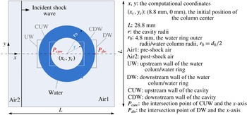
A schematic diagram of the shock wave interaction with a cylindrical water column embedded with a cavity is shown in figure 1, referring to the experiment and numerical simulations of Igra & Takayama (Reference Igra and Takayama2001a
,Reference Igra and Takayama
b
), Meng & Colonius (Reference Meng and Colonius2015).
 $r/r_{0}$
is the radius ratio between the coaxial water column and embedded cavity. If
 $r/r_{0}=0$
, the problem degenerates to the interaction of a planar shock with a cylinder water column. We use UW, DW, CUW and CDW to represent the nomenclature of water column/ring upstream wall, water column/ring downstream wall, downstream cavity wall and upstream cavity wall respectively. The schematic positions of UW, DW, CUW and CDW are also shown in figure 1.
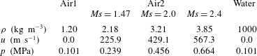
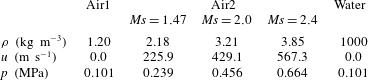
The parameters in the present simulations are shown in table 1.
 $\mathit{Ms}$
is the Mach number of the incident shock wave and
 $p$
is the pressure behind the incident shock wave. The Weber numbers in the present numerical simulations are taken as higher than 1000 and the corresponding Reynolds numbers are over 40 000. Therefore, the viscous effect and surface tension can be neglected in the numerical simulations (Meng & Colonius Reference Meng and Colonius2015).
2.2 Quasi-conservative interface model
In this paper, the fluids are assumed to be compressible without considering the flow viscosity and surface tension, and thus the two-phase flow is described by the conservative Euler equations, reading as,
 $$\begin{eqnarray}\frac{\unicode[STIX]{x2202}U}{\unicode[STIX]{x2202}t}+\frac{\unicode[STIX]{x2202}F(U)}{\unicode[STIX]{x2202}x_{j}}=0,\end{eqnarray}$$
where,
 $U=(\unicode[STIX]{x1D70C},\unicode[STIX]{x1D70C}u_{i},E)$
are the conservative variables including the mass density
 $\unicode[STIX]{x1D70C}$
, momentum
 $\unicode[STIX]{x1D70C}u_{i}$
(in the
 $i$
th direction) and the total energy
 $E=\unicode[STIX]{x1D70C}e+\unicode[STIX]{x1D70C}u_{i}u_{i}/2$
. Here,
 $e$
is the specific internal energy.
 $F(U)=[\unicode[STIX]{x1D70C}u_{j},\unicode[STIX]{x1D70C}u_{i}u_{j}+p\unicode[STIX]{x1D6FF}_{ij},(E+p)u_{j}]$
are the convective fluxes. The two-phase fluid respects the same stiffened gas equation of state (EOS) as
 $$\begin{eqnarray}\unicode[STIX]{x1D70C}e=\frac{p+\unicode[STIX]{x1D6FE}P_{\infty }}{\unicode[STIX]{x1D6FE}-1},\end{eqnarray}$$
Schematic diagram of the physical model and computational domain.

Set-up parameters for the numerical simulation cases.
where
 $\unicode[STIX]{x1D6FE}$
is the specific heat ratio and
 $P_{\infty }$
is the reference parameter with the dimension of pressure. Following the work of Allaire, Clerc & Kokh (Reference Allaire, Clerc and Kokh2002) and Johnsen & Colonius (Reference Johnsen and Colonius2006), because the material properties
 $\unicode[STIX]{x1D6FE}$
and
 $P_{\infty }$
are characterized in each phase, the diffusive interface can be resolved by the transport of such physical variables (Johnsen & Colonius Reference Johnsen and Colonius2006; Coralic & Colonius Reference Coralic and Colonius2014). The material properties follow the non-conservative equations
 $$\begin{eqnarray}\frac{\unicode[STIX]{x2202}\unicode[STIX]{x1D719}}{\unicode[STIX]{x2202}t}+\frac{\unicode[STIX]{x2202}(\unicode[STIX]{x1D719}u_{j})}{\unicode[STIX]{x2202}x_{j}}=\unicode[STIX]{x1D719}\frac{\unicode[STIX]{x2202}u_{j}}{\unicode[STIX]{x2202}x_{j}},\end{eqnarray}$$
where
 $\unicode[STIX]{x1D719}$
is given by
 $\unicode[STIX]{x1D719}=(\unicode[STIX]{x1D719}_{1},\unicode[STIX]{x1D719}_{2})^{\text{T}}=(1/(\unicode[STIX]{x1D6FE}-1),\unicode[STIX]{x1D6FE}P_{\infty }/(\unicode[STIX]{x1D6FE}-1))^{\text{T}}$
, with superscript T denoting the transpose.
The value of
 $\unicode[STIX]{x1D6FE}$
is 1.4 for air and 6.12 for water.
 $P_{\infty }$
is 0 for air and 0.343 GPa for water in the numerical simulation. With the Eulerian conservative law and the non-conservative transport equations of material properties, a quasi-conservative interface model is formed for the further numerical discretizations.
2.3 Numerical method and verification
A finite-volume method is applied to discretize the above governing equations in an uniform Cartesian grid system. Referring to the work by Johnsen & Colonius (Reference Johnsen and Colonius2006) and Coralic & Colonius (Reference Coralic and Colonius2014), the spatial discretization is based on Godunov-type methods. The Harten–Lax–van Leer Contact (HLLC) approximate Riemann solver is applied to solve the numerical fluxes and velocities required by (2.5) at the cell faces. A fifth-order incremental weighted essentially non-oscillatory (WENO) reconstruction combined with multidimensional optimal order detection (MOOD)-type positivity preservation, as previously proposed by the present authors (Wang et al. Reference Wang, Xiang, Zhang and Hu2016), are used to reconstruct the initial conditions for the Riemann problem at the cell face by characteristic primitive variables. The third-order total variation diminishing (TVD) Runge–Kutta method is employed to advance the solutions over time. The parallelization of the present simulation code based on the message-passing interface (MPI) enables the computation of the large-scale domain and long duration problems. The procedure to set up the initial shock wave conditions follows the below steps. Firstly, a simple Riemann problem of the gas is solved, in which the shock condition is the same as the selected cases in our numerical study. After some time, the shock wave will develop and diffuse across a few cells. Then, the data which diffuse across a few cells will be extracted to set up the initial shock wave conditions.
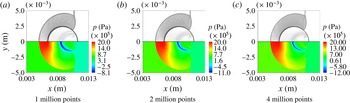
The schlieren (top) and pressure (bottom) contours of the three different mesh levels at
 $t^{\ast }=0.80$
,
 $Ms=2.4$
.

In the following, the non-dimensional time is used for further analysis, which is given by
 $$\begin{eqnarray}t^{\ast }=\frac{tu_{2}^{\prime }}{d_{0}},\end{eqnarray}$$
where
 $t$
is the physical time and
 $u_{2}^{\prime }$
is the initial velocity behind the incident shock.
 $d_{0}$
represents the initial diameter of the water column or the outer diameter when a cavity is embedded inside.
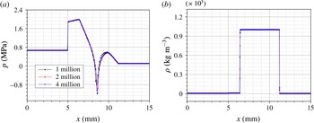
Three cases of different grid resolution varying from 1 to 4 million grid points are employed to validate the grid sensitivity computation. Figure 2 shows the schlieren (top) and pressure (bottom) contours at the fixed non-dimensional time
 $t^{\ast }=0.80$
. The shock wave structures and two-phase interfaces become sharper when the grid resolution is enhanced. At the same time instant, the pressure and density along the axial line are shown in figure 3(a,b). The density profiles along the axial line show no evident differences between the three chosen grid resolutions. It is observed from figure 3(a) that the pressure has negative values in the region of the expansion wave, which are allowed in numerics since the stiffened gas EOS is used and the phase transition is not considered (Sembian et al.
Reference Sembian, Liverts, Tillmark and Apazidis2016). The pressure profiles along the axial line overlap well for higher grid resolutions, except for a slight variation of the negative peak pressure, which will not affect the following analysis for the current investigation. Thus, in the present subsequent analysis, the refined 4 million grid level is chosen to accomplish the simulations. The grid resolution remains unchanged for all the simulation cases in the paper and the details can refer to the simulations cases in §§ 3 and 4.
The pressure (a) and density (b) along the axial line of the three different mesh levels at
 $t^{\ast }=0.80$
,
 $Ms=2.4$
.

3 Water column without an interior cavity
The interaction of a planar shock wave with a single cylindrical water column has been investigated by researchers through experiments and numerical simulations. Comparing the present simulation results with those obtained in Sembian et al. (Reference Sembian, Liverts, Tillmark and Apazidis2016), Meng & Colonius (Reference Meng and Colonius2015), the reliability of the present simulation code is shown. In this section, half of the domain is computed. For the lower wall, the symmetric boundary condition is employed, while the other walls use the non-reflection characteristic boundary condition. For the water column, the cell number across the column diameter is 333, which is sufficient to provide detailed flow structures.
Numerical schlieren contours (top) and pressure contours (bottom) at different time intervals for
 $Ms=2.4$
. Also shown on the right-hand side of (a–f) are the results from Sembian et al. (Reference Sembian, Liverts, Tillmark and Apazidis2016).

3.1 Qualitative analysis
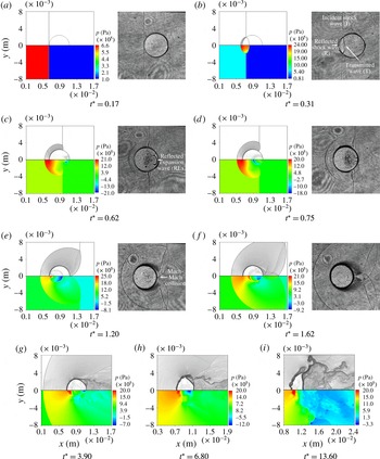
The numerical schlieren and pressure contours are shown in figure 4 for the case of
 $Ms=2.4$
, where the plugged grey schlieren contours (the right-hand side of figure 4
a–f) are the flow visualizations from the experiment of Sembian et al. (Reference Sembian, Liverts, Tillmark and Apazidis2016). When the incident shock wave impinges on the water column, it is reflected off the UW of the water column and transmitted into the liquid. Then, the reflected shock wave interacts with the incident shock wave. A slip line occurs subsequently, and there is a triple point. As the speed of sound in water is much higher than that in the air, the transmitted wave quickly reaches the DW of the water column. When the transmitted wave arrives at the furthest point of the DW of the water column, the expansion wave will focus near this point inside the water column. Then, the expansion wave will propagate towards the UW of the water column and will be reflected inside the water column repeatedly. In the meanwhile, the transmitted wave is re-transmitted into the air and forms the re-transmitted wave. This re-transmitted wave is a kind of weak compression wave because the transmitted wave inside the water column is damped when it is transmitted into the air passing through the curved surface of the water column. The increased pressure ratio of this wave is approximately 1.0067 and the increased density ratio is approximately 1.0048 when the incident shock Mach number is 2.4.
Since the water column is not a streamlined geometry, the induced flow around the water column cannot recover its static pressure behind the water column when it is impinged by a planar shock wave. Then, the flow will separate, and the separated vortex will entrain the surrounding air. Thus, the recirculation region is formed, which will prevent the DW of the water column from moving toward the right side. This ‘blocking effect’ will be much stronger near the rear stagnation point, where the surrounding flow pulls away the air from the equator. Meanwhile, the centre of mass of the water column moves towards the right due to the impaction of the incident shock wave. Thus, the water column seems to be squeezing continuously and the DW of the water column becomes flattened, as shown in figure 4(g–i). In the work of Meng & Colonius (Reference Meng and Colonius2015) a similar phenomenon is observed.
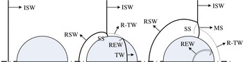
The wave structures at the early stages of the shock/droplet interaction are typically used to validate the numerical schemes as in Ball et al. (Reference Ball, Howell, Leighton and Schofield2000), Sembian et al. (Reference Sembian, Liverts, Tillmark and Apazidis2016). Fundamentally, typical waves are extracted in the present study and shown in figure 5. Only the early stages of the evolution of the interaction of a planar shock wave with a cylindrical water column are presented here.
When an incident shock wave moves across a water column from the left to the right side, the transmitted wave and reflected shock wave occur simultaneously, and subsequently, the reflected shock wave propagates upstream into the surrounding air and the transmitted wave propagates downstream inside the water column. The transmitted wave will be re-transmitted into the downstream air when it reaches the DW of the water column. The expansion waves will be reflected inside the water column again and again. Above the lateral pole of the water column, the incident shock wave, the Mach stem and the slip line form the triple point. These wave structures, as well as the two-phase interface, are the typical flow characters in the early stages of the shock/droplet interaction and emerge as discontinuities with different intensities, which pose challenges to numerical schemes.
Schematic diagram of the wave structures of a planar shock wave interacting with a water column (ISW: the incident shock wave; RSW: the reflected shock wave; TW: the transmitted wave; REW: the reflected expansion wave; R-TW: the re-transmitted wave; SS: the slip surface; MS: the Mach stem).

Micro-mist is observed in the experiments of Wierzba & Takayama (Reference Wierzba and Takayama1988), Sembian et al. (Reference Sembian, Liverts, Tillmark and Apazidis2016). This may be caused by liquid atomization and evaporation in later stages. In the numerical simulations, the heat conduction and viscous effects were not considered, as is the case for most numerical simulations in the literature. Currently, the simulation results are viable to evaluate the possibility of the atomization and evaporation of the liquid droplet. Through the post-processing, the temperature can be obtained. In our numerical model, the stiffened equation of state is used and it does not give the explicit expression of the temperature. Thus, the temperature is computed in the following way. The specific heat ratio
 $\unicode[STIX]{x1D6FE}$
is identified to distinguish the air and the water. For the air, it is treated as a calorically ideal gas and the temperature is computed via the thermal equation of state, which has the simple expression
 $$\begin{eqnarray}T_{g}=\frac{pv}{R},\end{eqnarray}$$
where
 $T_{g}$
is the gas temperature and
 $R$
is the gas constant, which is
 $287.05~\text{J}~\text{kg}^{-1}~\text{K}^{-1}$
for air.
 $p$
is the pressure at a cell and
 $v$
is the specific volume, which is equivalent to
 $1/\unicode[STIX]{x1D70C}$
. For the water, the magnitude of the pressure variation is far less than the liquid parameter
 $P_{\infty }$
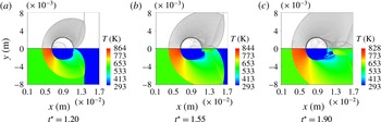
. Thus, the temperature variation of the water induced by the pressure and density variation can be neglected. Then, the water temperature is assumed as the unchanged initial temperature, 293 K. Figure 6 shows the temperature and schlieren contours at three time instants when
 $Ms=2.4$
. The temperature of the upstream air is approximately 870 K near the upward stagnant point according to the numerical results.
In order to evaluate the effect of evaporation, an energy balance idea is introduced similar to the treatment of Klein et al. (Reference Klein, Bouwhuis, Visser, Lhuissier, Sun, Snoeijer, Villermaux, Lohse and Gelderblom2015). To vaporize a certain fraction of a droplet, the energy transferred from the air should balance the internal energy increase and the latent heat of the vaporization of the liquid as below
 $$\begin{eqnarray}\unicode[STIX]{x1D70C}_{l}[r_{0}^{2}-(r_{0}-\unicode[STIX]{x1D6FF}_{l})^{2}][c_{v}^{l}(T_{b}-T_{0})+\unicode[STIX]{x0394}H]=\unicode[STIX]{x1D70C}_{g}[(r_{0}+\unicode[STIX]{x1D6FF}_{g})^{2}-r_{0}^{2}]c_{v}^{g}(T_{g}-T_{b}),\end{eqnarray}$$
where
 $\unicode[STIX]{x1D70C}_{l}$
and
 $\unicode[STIX]{x1D70C}_{g}$
are the water and air densities;
 $\unicode[STIX]{x1D70C}_{l}$
is chosen to be
 $1000~\text{kg}~\text{m}^{-3}$
;
 $\unicode[STIX]{x1D70C}_{g}$
is set as the post-shock density with
 $Ms=2.4$
, namely
 $\unicode[STIX]{x1D70C}_{g}=3.85~\text{kg}~\text{m}^{-3}$
.
 $r_{0}$
is the column initial radius.
 $c_{v}^{l}$
and
 $c_{v}^{g}$
are the specific heat capacities of the water and the air and the values are
 $4.2~\text{kJ}~\text{kg}^{-1}~\text{K}^{-1}$
and
 $0.717~\text{kJ}~\text{kg}^{-1}~\text{K}^{-1}$
, respectively. The right-hand side of (3.2) represents the maximum energy which is transferred from the surrounding air layer (here denoted as
 $\unicode[STIX]{x1D6FF}_{g}$
) to the water column. The energy can be calculated assuming the fast equilibrium process of the vaporization. The left side of (3.2) represents the energy to heat of the liquid phase from the ambient temperature
 $T_{0}=293~\text{K}$
to the boiling temperature
 $T_{b}=393~\text{K}$
as well as the latent heat the vaporization of the water
 $\unicode[STIX]{x0394}H=2.25~\text{MJ}~\text{kg}^{-1}$
(Klein et al.
Reference Klein, Bouwhuis, Visser, Lhuissier, Sun, Snoeijer, Villermaux, Lohse and Gelderblom2015). In (3.2),
 $T_{g}$
is chosen as the highest temperature of the air, which is 870 K near the upward stagnant point;
 $\unicode[STIX]{x1D6FF}_{g}$
is chosen as
 $0.25r_{0}$
,
 $0.5r_{0}$
,
 $1.0r_{0}$
,
 $1.5r_{0}$
and
 $2.0r_{0}$
to check the effects of the thickness of the aerothermal layer on the possible evaporation of the water column (the thickness of the evaporated liquid layer is denoted as
 $\unicode[STIX]{x1D6FF}_{l}$
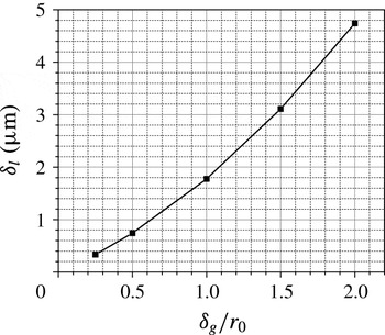
). The results are shown in figure 7. The evaporated liquid layer is too thin. As shown in figure 7,
 $\unicode[STIX]{x1D6FF}_{l}$
is
 $4.739~\unicode[STIX]{x03BC}\text{m}$
for
 $\unicode[STIX]{x1D6FF}_{g}=2r_{0}$
. Thus, the column breakup cannot be concluded by the possible evaporation due to aerothermal heating.
Numerical schlieren contours (top) and temperature contours (bottom) at different time intervals,
 $Ms=2.4$
.

Effects of different thickness of the aerothermal layer on possible evaporated liquid layer (
 $\unicode[STIX]{x1D6FF}_{l}$
) of the water column.

3.2 Parameter study
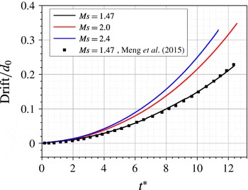
Firstly, the acceleration process of the water column under different incident shock intensities is analysed. Therefore, the drift of the water column is needed. In this paper, the drift is obtained by finding the location of the mass centre according to Meng & Colonius (Reference Meng and Colonius2015), as shown below:
 $$\begin{eqnarray}\bar{\boldsymbol{x}}=\frac{\displaystyle \int _{S}\unicode[STIX]{x1D70C}_{l}\boldsymbol{x}\,\text{d}x\,\text{d}y}{\displaystyle \int _{S}\unicode[STIX]{x1D70C}_{l}\,\text{d}x\,\text{d}y},\end{eqnarray}$$
where
 $\unicode[STIX]{x1D70C}_{l}$
is the liquid density and the integral volume is the whole two-dimensional computational domain. The drift of the water column is normalized by the initial column diameter,
 $d_{0}$
. The post-process results are shown in figure 8. The stronger the incident shock wave, the faster the column moves. The total drift of the present three computational case is within 0.4 column diameters. As time advances, the drift of the mass centre accumulates nonlinearly. The drift of the centre of mass from the paper of Meng & Colonius (Reference Meng and Colonius2015) is also shown in figure 8 in the case of
 $Ms=1.47$
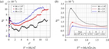
. It is observed that the curve almost overlaps with the result of Meng & Colonius (Reference Meng and Colonius2015). The acceleration history of the centre of mass is evaluated based on the drift, as shown in figure 9. In figure 9(a), the acceleration is normalized by the initial diameter of the water column and the velocity of the post-shock air. A peak acceleration occurs shortly after the incident shock wave impacts on the water column. In the case of
 $Ms=1.47$
, the acceleration will oscillate at later times, while for the higher incident Mach numbers this is not obvious. The shedding vortex behind the water column can explain this, and for lower incident Mach numbers, the effect of the shedding vortex is more prominent. In figure 9(b), the acceleration in figure 9(a) is rescaled by the pressure ratio across the incident shock wave. It is obvious from figure 9(b) that the rescaled acceleration is larger for lower incident Mach numbers. The peak acceleration shortly after the incident shock impacts on the water column is given in figure 9(b) and it is of the order of
 $10^{5}~\text{m}~\text{s}^{-2}$
. This value increases when the incident Mach number increases.
The drift of the mass centre.

The acceleration process of the centre of mass.

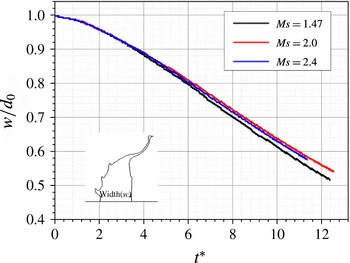
The deformation parameters of the water column are characterized by the width in the central line and the spanwise height. Figure 10 shows the column centreline width normalized by the initial column diameter. The water column centreline width will decrease with increasing time for each Mach number. The higher intensity shock will lead to a faster decrease in speed.
The centreline width of the water column.

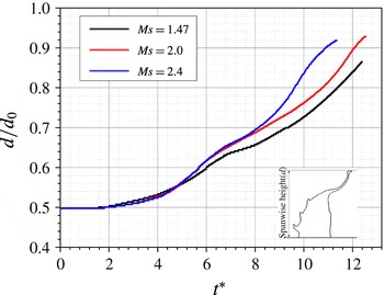
Figure 11 shows the spanwise height of the water column, which is normalized by the initial column diameter. It can be seen that the spanwise height can increase by 0.93 times the initial column diameter. The speed first increases and then decreases. Finally, the spanwise height will reach its peak value as the liquid strips off the liquid column from our previous analysis. The spanwise height of the water column remains unchanged irrespective of the incident shock intensity during the initial stages, which indicates a weak deformation of the water column. Then it will increase quickly followed by a plateau over a very short period of time, i.e. a very slow increase of height. Afterward, the column height continues to increase.
The spanwise height of the water column.

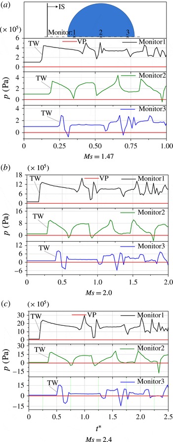
In the present numerical simulations, three typical monitor points that were spatially mounted to detect the pressure are shown in figure 12(a). The pressures at these points are illustrated in figure 12(a–c). Because the locations of the monitor points are fixed in space, only the early stages of the evolution are valid for detecting the pressure in the water column.
The pressure variation at each monitor point has a similar trend for the three incident shock intensities. The pressures initially increase sharply as the transmitted wave passes these monitor points in sequence. Then, the expansion wave will propagate towards the UW of the water column. The pressure at monitor point 3 will firstly experience a valley value because of the expansion wave. It is also found in figure 12 that the first valley pressure gets lower for the monitor points 2 and 3 when the incident shock intensity increases from
 $Ms=1.47$
to
 $Ms=2.4$
. The reason is that the expansion wave will get stronger as the focusing effect is stronger for larger incident Mach number near the DW of the water column. The intensity of the expansion wave will become weaker as it propagates from the right to the left. Thus, the first valley pressure decreases from the monitor point 3 to the monitor point 1. At later times, the pressure at the three monitor points will experience several peaks and valleys as the expansion wave reflects inside the water column again and again. Compared with the saturation vaporization pressure (VP), which is 2339 Pa for the liquid water at the temperature 293 K, it is observed from figure 12 that the valley pressures are above the value of VP at monitor 1 for the three incident shock intensities in the numerical simulations. For the low incident Mach number, i.e.
 $Ms=1.47$
, the pressure at monitor points 2 and 3 will suddenly drop below the vaporization pressure several times. However, these valley pressures are not low enough and they only occur during an extremely short time, which indicates that the possibility of cavitation is low for this case. For lager incident Mach numbers, i.e.
 $Ms=2.0$
and
 $Ms=2.4$
, the valley pressure at monitor 3 has the value that below VP more frequently. For the case of
 $Ms=2.4$
, the low pressure below the VP lasts for a longer period of time. This result indicates that there is a higher possibility for cavitation of the fluid near the DW of the water column. The present numerical results are consistent with the experimental observations in Sembian et al. (Reference Sembian, Liverts, Tillmark and Apazidis2016).
The pressure variations at three different locations (IS: the incident shock wave; TW: the transmitted wave; VP: the saturation vaporization pressure).

4 Water column embedded with a cavity
The possibility of cavitation is found when the water column is impinged by a high intensity shock wave, as shown above. In this section, the interaction of a planar shock wave with a water column embedded with a cavity is studied. Three cases are simulated with different cavity sizes of the air phase, as characterized by the radius ratio
 $r/r_{0}$
from 0.25, 0.5 to 0.75. The cell number across the liquid of the water ring is 83, 166 and 250, corresponding to
 $r/r_{0}=0.75,0.5$
and
 $0.25$
, respectively.
4.1 Qualitative analysis
When a planar shock wave interacts with a water ring, the wave structures is complicated and the water ring has a large deformation. As similarly done by Hawker & Ventikos (Reference Hawker and Ventikos2012), the entire process of a planar shock wave interacting with a water ring is also defined as three stages based on the dominant factors , i.e. significantly different flow characteristics observed in each stage. The main difference for the different Mach numbers is that the duration of the three stages is different. Thus, only the case of
 $Ms=2.4$
and
 $r/r_{0}=0.75$
is chosen to illustrate the instantaneous evolution.
4.1.1 First stage evolution
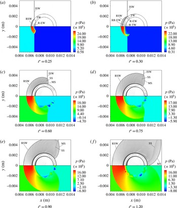
The first stage begins as the incident planar shock wave comes into contact with the UW of the water ring, as shown in figure 13. During the first stage, the geometrical configuration of the water column remains unchanged and the wave structure is clear. When a planar shock wave from the air impinges on a water ring, it will be reflected at the UW and transmitted into the water ring. This forms the first transmitted wave. Later on, the first transmitted wave will be transmitted and reflected again when it contacts with the CUW. Then, the transmitted wave is captured once more inside the cavity. As the reflection and transmission repeat again and again inside the liquid of the water ring, multiple transmitted waves occur in the cavity, as shown in figure 11(b–f). Due to the curvature effect of the cavity, the transmitted waves are observed as round-shape waves. When the Mach number of the incident shock wave is 2.4 and
 $r/r_{0}$
is 0.75, it is calculated that the transmitted wave inside the liquid can be reflected 4 times at the CUW from
 $t^{\ast }=0.25$
to
 $t^{\ast }=0.60$
. In figure 11(c), 4 round-shape compression waves are identically observed inside the cavity correspondingly. As the incident shock wave propagates downstream, the Mach stem and the slip line are found in figure 13(c–f).
The first stage of the evolution of the planar shock wave interacting with a water ring,
 $Ms=2.4$
. Numerical schlieren contours (top); pressure contours (bottom) (ISW: the incident shock wave; RSW: the reflected shock wave; TW: the transmitted wave; R-EW: the reflected expansion wave; R-TW: the re-transmitted wave; RR-EW: the re-reflected expansion wave; SS: the slip line; MS: the Mach stem).

4.1.2 Second stage
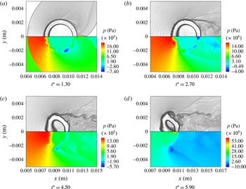
The second stage begins as the water column deforms significantly and ends as the liquid jet impacts on the CDW, as shown in figure 14. The upstream air pressure is further increased because of the reflected shock wave. There is a low pressure region behind the DW of the water ring because of the flow recirculation. The DW of the water ring is flattened for the same reason as the planar shock interacting with a water column (see § 3.1). The most significant flow phenomenon observed in the second stage is the transverse jet. The formation mechanism is explained as below. Firstly, the Richtmyer–Meshkov instability will occur when the round liquid/air interface is impinged by a planar shock wave. As the Richtmyer–Meshkov instability develops, the heavy liquid will be driven into the light fluid. Secondly, when the incident shock wave impinges on the water ring, the pressure of the left side ring will increase. Then, due to the pressure gradient, the liquid of the left side water ring will also be driven into the cavity. In addition, due to the curvature effect, the liquid that is closer to the centreline will go faster than the liquid far from the centreline. Based on the above reason, the liquid of the left side water ring is forced to move toward the right side and involutes to form the transverse jet. Finally, the jet impacts on the CDW. The air inside the cavity is highly compressed and the peak pressure occurs at the tip region of the transverse jet.
The second stage of the evolution of the planar shock wave interacting with a water ring,
 $Ms=2.4$
. Numerical schlieren contours (top); pressure contours (bottom).

4.1.3 Third stage
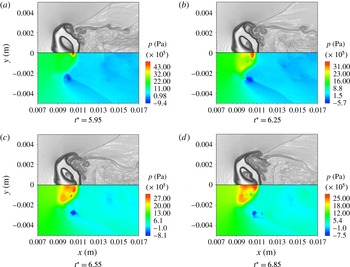
The third stage begins as the transverse jet impacts on the CDW, as shown in figure 15. The peak pressure decreases with time, but the pressure of the liquid jet increases. Unlike the collapse of an air bubble in the ambient liquid medium referred to in Hawker & Ventikos (Reference Hawker and Ventikos2012), water hammer shock is not found when the transverse jet impacts on the CDW, even if the incident Mach number is increased to 2.4 in the present study because of the momentum exchange between the transverse jet and downstream water ring. In this stage, the dominant factor is the interaction of the transverse jet with the CDW. The DW of the water ring begins to move towards the right side because of the high momentum transverse jet, and this relaxes the high pressure caused by the impaction of the transverse jet on the CDW.
The third stage of the evolution of the planar shock wave interacting with a the water ring,
 $Ms=2.4$
. Numerical schlieren contours (top); pressure contours (bottom).

4.2 Morphology
The morphology is analysed in the deforming process of the cylindrical water column embedded with a cavity impinged by a planar shock wave. Figure 16 shows the isolines of the specific heat ratio
 $\unicode[STIX]{x1D6FE}$
, which is used to show the interface spatio-temporal evolution for the case of
 $Ms=2.4$
,
 $r/r_{0}=0.75$
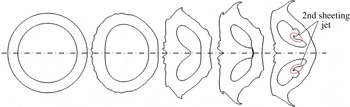
. Initially, the shape of the cylindrical water column with a cavity embedded looks like a water ring. Later on, the left side of the water ring deforms and the cavity inside is slightly compressed. Interface instability occurs at the UW of the water ring. Then, the transverse jet gradually forms and the liquid of the spanwise pole strips off the water ring. Meanwhile, the DW of the water ring is forced to move towards the cavity side. Next, the transverse jet hits on the CDW and the DW of the water ring is forced to moves toward the right side because of the momentum exchange with the transverse jet. The volume of the cavity decreases, also shown in figure 16, because the air is significantly compressed. For larger incident shock intensity, when the transverse jet impacts on the CDW, an extremely high pressure region will be formed near the impaction point. Due to the high pressure gradient, the fluid is driven into the cavity, forming a sheeting jet, which can be called as the second sheeting jet following the description in Hawker & Ventikos (Reference Hawker and Ventikos2012). This sheeting jet is demonstrated in figure 16. But for the lower Mach number, the sheeting jet is not found, which is not shown in the present analysis. The reason is that the intensity of the transverse jet is weak for the low
 $Ms$
case. The pressure around the impaction point cannot be elevated very high. For instance, for the case of
 $Ms=1.47$
, the pressure is about 0.4 MPa in the region where the transverse jet impacts on the CDW. The pressure is not high enough to drive the fluid into the cavity.
The interface shape evolution of the planar shock wave interacting with the water ring,
 $Ms=2.4$
.

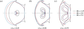
The shapes of the deforming water column are plotted in figure 17 when the transverse jet impacts on the CDW for different incident shock intensities and radius ratios. In case of
 $Ms=1.47$
, the transverse jet is weak. Thus the cavity is less compressed and the cavity volume slightly changes. As the shock intensity increases, the cavity deforms significantly when the transverse jet impacts on the CDW. The shape of the deformed cavity is somehow like a pair of symmetric kidney. For the case of
 $r/r_{0}=0.25$
, at the time when the transverse jet hits the CDW, the centreline width of the water ring is smaller for a weaker incident shock wave. When
 $r/r_{0}$
is 0.5, the outer wall shape of the water ring is similar and the transverse jet width is larger with a stronger incident shock wave. When
 $r/r_{0}$
is 0.75, the transverse jet width is approached for
 $Ms=2.0$
and
 $2.4$
, but longer than that of
 $Ms=1.47$
.
In the work of Koukouvinis et al. (Reference Koukouvinis, Gavaises, Supponen and Farhat2016), both the experimental and numerical results show that the jet becomes like a needle when it pierces the bubble for the problem of bubble collapse under gravity. In our numerical study, when a cavity-embedded water column is impacted by an incident shock wave, it is found that the transverse jet resembles a ‘spike’ as the cavity collapse. The width of the jet tip is larger for higher incident shock intensities when the transverse jet impacts on the CDW. However, for lower incident shock intensities and smaller cavity sizes, i.e.
 $Ms=1.47$
and
 $r/r_{0}=0.25$
, the jet is thinner and becomes like a needle.
The interface shape at the time when the transverse jet impacting on the CDW for different Mach numbers and radius ratios.

4.3 Parameter study
As observed in the qualitative analysis above, the collapse of the cavity inside the water column by an incident shock wave will lead to a strong compression of the air inside. Taking the case of
 $Ms=2.4$
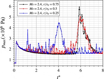
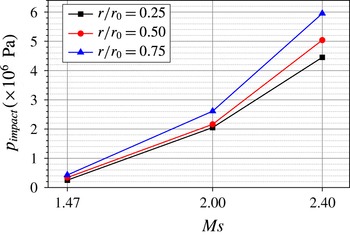
as an example, figure 18 shows the maximum pressure of the whole computational domain. From the maximum pressure curves over time, the maximum peak pressure is obtained for each radius ratio. Corresponding to the qualitative observation, the maximum peak pressure occur as the first transverse jet (also called the main transverse jet) just impacts on the CDW. However, this observation is only validated for larger incident shock intensities. Though the numerical simulation results are not presented here for lower incident shock intensities, it is addressed that the transverse jet is weaker. When the transverse jet just impacts on the CDW, the pressure near the impaction point will not be elevated high enough. The peak pressure (
 $p_{impact}$
) near the impaction point when the transverse jet just impacts on the CDW under different
 $Ms$
and
 $r/r_{0}$
is shown in figure 19. For the case of
 $Ms=1.47$
, the transverse jet is weak. The peak pressure near the impaction point is approximately 2.5 to 4.3 times that of the initial cavity pressure. For the case of
 $Ms=2.0$
, the peak pressure is approximately ranged from 2.0 to 3.6 MPa, which is about 20 to 26 times the initial pressure inside the cavity. When the shock wave intensity increases, the peak pressure increases. The peak pressure also increases as the cavity size becomes larger. The highest peak pressure can reach approximately 5.95 MPa in case of
 $Ms=2.4$
and
 $r/r_{0}=0.75$
, which is 59 times the initial pressure inside the cavity.
The maximum pressure of the whole computational domain over time of different radius ratios,
 $Ms=2.4$
.

The peak pressure near the impaction point of different Mach numbers and radius ratios.

The centreline pressure and density profiles at the time when the transverse jet impacts on the CDW.

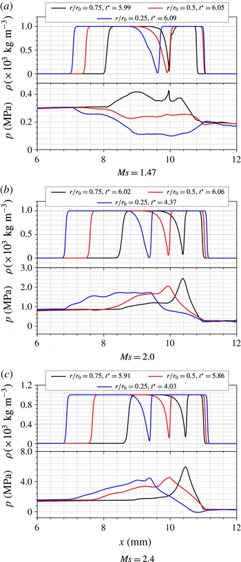
Figure 20 shows the centreline pressure and density profiles for different incident shock intensities and cavity radii. The cuspidal shape of the density means that the transverse jet just impacts on the CDW. It is observed from figure 20(b,c) that the pressure profiles along the centreline are similar and a peak pressure occurs at the impaction point for larger incident shock intensities. That means the air between the tip of the transverse jet and the CDW is highly compressed for larger cavity radius ratios when the incident shock wave intensity is high. However, in figure 20(a), it is found that the overall behaviour of the pressure curves of the cases
 $r/r_{0}=0.25$
and
 $0.5$
is significantly different from that of
 $r/r_{0}=0.75$
. The pressure inside the water ring is lower than that in the upstream air along the centreline. Whereas, in case of
 $r/r_{0}=0.75$
, the pressure inside the water ring is larger than that in the upstream air along the centreline. This can be explained as below. The transverse jet is weaker for smaller radius ratios, and the pressure has no augmentation in the region between the UW of the water ring and the CDW but is relaxed before the jet impacts on the CDW. In the case of
 $r/r_{0}=0.75$
, the transverse jet is stronger than those of
 $r/r_{0}=0.25$
and
 $0.5$
, and the pressure is augmented because of faster compression imposed by the jet. Therefore, the pressure increases along the centreline in the water ring. Moreover, just because the air is fast compressed when the jet tip is closer to the CDW, there exists a local pressure peak near the impaction point (around
 $x=10.0~\text{mm}$
) in the flow field of the case
 $r/r_{0}=0.75$
.
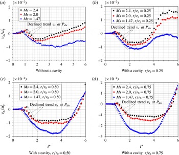
The normalized
 $x$
-velocity component at the tracking point
 $P_{dw}$
for different Mach numbers and radius ratios.

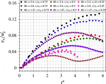
The normalized
 $x$
-velocity component at the tracking point
 $P_{cuw}$
for different Mach numbers and radius ratios.

When a planar shock wave interacts with a water column, the impaction of the incident shock will accelerate the water column to move toward the right side. Meanwhile, the trailing shedding vortex will prevent the water column from moving toward the right side. Both the acceleration effect and blocking effect will influence the motion of the DW of the water column. Figure 21(a) shows the temporal variation of the
 $x$
-velocity component (
 $v_{x}$
) at
 $P_{dw}$
. It is observed from this figure that
 $v_{x}$
at
 $P_{dw}$
first increases to the peak value. The higher the incident shock intensity is, the larger the peak value of
 $v_{x}$
is. The reason is that the acceleration effect dominates the motion of the water column in the early stages as the trailing shedding vortex has not been formed in this period. The later declined trend again indicates that the DW of the water column is forced to move towards the left by the trailing shedding vortex. It is the blocking effect overwhelms the acceleration effect that counts for this. Later on,
 $v_{x}$
seems to have a stable value in a very short duration, which means that the blocking effect is in balance with the acceleration effect. Finally, the acceleration effect will exceed the blocking effect and
 $v_{x}$
goes up. For all the cases of the water ring, the similar declined trends are observed for different incident shock wave intensities, as shown in figure 21(b–d). This can be explained similarly with the dynamical process of the shocked water column. However, the durations of the stable value of
 $v_{x}$
are much longer than that of the water column for each incident shock wave intensity. This can be resulted from the prolonged balance effect because of the existence of the embedded cavity inside the water column. It is known that the transverse jet can accelerate the downstream liquid when it interacts with the CDW. As the radius of the cavity increases, the transverse jet is strong enough even for lower incident shock intensity and the DW of the water ring will accelerate quickly after the impact of the transverse jet. Therefore, after the period of the stable value,
 $v_{x}$
will accumulate quickly especially for larger radius ratios.
The temporal variation of the
 $x$
-velocity component at the tracking point
 $P_{cuw}$
is identified and shown in figure 22, the initial position of which is shown figure 1. The velocities are recorded until the transverse jet impacts on the CDW. That means the recording time covers the first and the second stage as proposed in § 4.1. Both the overall movement of the water ring and the formation of the transverse jet can be also analysed based on the
 $x$
-velocity component at
 $P_{dw}$
(shown in figure 21) and
 $P_{cuw}$
(shown in figure 22). It is observed that
 $v_{x}$
at
 $P_{dw}$
is much smaller than that at
 $P_{cuw}$
. This means that the upstream fluid moves faster towards the DW of the water ring and also means that the transverse jet will form gradually. Once the jet is formed,
 $v_{x}$
at
 $P_{cuw}$
represents the jet tip velocity. It is noticed that there is a declined trend for
 $v_{x}$
at
 $P_{cuw}$
just before the jet tip comes into contact with the CDW for larger cavity radius. It means that the transverse jet gets weaker before it impacts on the CDW due to the reaction from the local highly compressed air. However, for the case of
 $Ms=1.47$
and
 $r/r_{0}=0.25$
,
 $v_{x}$
has a slowly ascending trend after the accelerating and decelerating periods before the jet impacts on the CDW. This is because of pressure relaxation of the transverse jet, which has been already discussed as aforementioned. The final point of each curve represents the jet tip velocity when the transverse jet just reaches the CDW. We call this velocity here as the jet impaction velocity. For the same initial incident shock intensity, the jet impaction velocity is higher as the cavity radius increases. The impaction of the transverse jet on the CDW is dramatic for higher incident shock intensities and larger cavity radius. For the case of
 $Ms=2.4$
and
 $r/r_{0}=0.75$
, the computed impaction velocity can reach up to
 $65~\text{m}~\text{s}^{-1}$
.
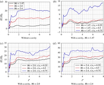
In similar to the work of Niederhaus et al. (Reference Niederhaus, Greenough, Oakley, Ranjan, Anderson and Bonazza2008), the enstrophy is evaluated for the interaction of the planar shock wave with the water column. The enstrophy is rewritten in a mass-averaged form, considering the flow compressibility of the highly compressible two-phase flow in our numerical study. The expression of
 $\unicode[STIX]{x1D6FA}$
is given as below,
 $$\begin{eqnarray}\unicode[STIX]{x1D6FA}=\frac{\displaystyle \int _{S}\unicode[STIX]{x1D70C}\unicode[STIX]{x1D714}^{2}\,\text{d}x\,\text{d}y}{\displaystyle \int _{S}\unicode[STIX]{x1D70C}\,\text{d}x\,\text{d}y},\end{eqnarray}$$
where
 $\unicode[STIX]{x1D70C}$
and
 $\unicode[STIX]{x1D714}$
are the density and vorticity at each cell, respectively. The values are integrated over the whole computational domain and normalized by a fixed value
 $\unicode[STIX]{x1D6FA}_{0}=10^{9}~\text{s}^{-1}$
. For the stronger incident shock intensity, the normalized enstrophy value is larger, on average. In case of
 $r/r_{0}=0.25$
and
 $r/r_{0}=0.5$
, compared to the variation of the enstrophy for the interaction of a planar shock wave with a water column, it is not significantly changed even if the cavity is embedded in the water column, as shown in figure 23(b–d).
The enstrophy evolution under different incident shock intensities and radius ratios.

It is observed from figure 23 that the trends of enstrophy are similar with each other for different incident shock intensities when
 $t^{\ast }$
is less than 1.8. They initially increase sharply, but then generally show an ascending trend with one peak value. During this period, the water column or the water ring does not deform significantly. It is the interaction between the complicated wave structures and the two-phase interface that generates the obvious baroclinic torque. This baroclinic mechanism contributes to the generation and drastic change of the enstrophy. When
 $t^{\ast }$
is larger than 1.8, the value of enstrophy tends to be stable in the case of
 $r/r_{0}=0.25$
and
 $0.5$
. However, for the case of
 $r/r_{0}=0.75$
of the water ring, the enstrophy still has large fluctuations for the low incident Mach number, since the water ring deforms significantly for larger radius ratio.
5 Summary
In this paper, the interactions of a planar shock wave with a cylindrical water column embedded with/without a cavity are numerically investigated. The conservative Eulerian and material properties transport equations consist of the diffusion interface capture model. The HLLC Riemann solver coupled with an incremental stencil WENO scheme is used to solve the numerical fluxes of the governing Euler equations. A third-order TVD Runge–Kutta scheme is used to advance the solution in time. The results show that the evolution of the wave structures and the morphology of the two-phase interface are consistent with the case of the shock interaction with single water column from the experiment in Sembian et al. (Reference Sembian, Liverts, Tillmark and Apazidis2016).
When the water column is shocked by a high intensity shock wave, the focusing of the expansion wave results in a sustained local low pressure near the rear water column wall, which indicates potential cavitation there. Theoretical analysis of the aerodynamic heating process surrounding the droplet shows that liquid aerodynamic atomization is the main reason for the formation of the micro-mist at later stages of the water column breakup. The deformation process of the two-phase interface of the water column at early stages is characterized by its streamwise and spanwise length scale, which demonstrates that the water column is elongated in the spanwise direction and flattened in the streamwise direction with time advancing, and the deformation rate of the water column varies nonlinearly with different incident Mach numbers.
The interaction of a planar shock with a water column embedded with a cavity then shows detailed evolutions of the wave structures and gas phase interface morphologies. Simulations are also conducted for different incident shock wave intensities and different sizes of the embedded cavity. The transverse jet is formed because of the interface instability of the CUW and the pressure gradient of the left side water ring, which are caused by the impaction of the incident shock. The
 $x$
-component velocities at the tracking points
 $P_{dw}$
and
 $P_{cuw}$
are extracted to analyse the interface evolution. The case of
 $Ms=2.4$
and
 $r/r_{0}=0.75$
has the largest relative impaction velocity when the transverse jet just impacts on the CDW. Under the same shock intensity, the momentum of the transverse jet increases when increasing the embedded-cavity radius in the water column.
Different from bubble collapse in water as in Hawker & Ventikos (Reference Hawker and Ventikos2012), the water hammer shock is not found when a cavity collapses inside a water column. Numerical analysis shows that it is the relaxing process of the accelerated right side liquid of the water ring that accounts for this phenomenon. The whole field enstrophy is compared to show that the increasing trend is characterized by the contributed generation of a vortex due to the baroclinic effects of the shock wave interacting on the two-phase interfaces.
In this study, the bubble is embedded in the central location of the water column. In future work, the dynamics of the eccentric located cavity will be studied to show bubble collapse. For an in-depth study, a realistic equation of state will also be considered in the numerical simulation.
Acknowledgements
The authors would like to thank the partial finical support from the Natural Science Foundation of China under the grant no. 51676111&11628206 and the Tsinghua University Initiative Scientific Research Program.