

Introduction
Affective polarization is the soup du jour in contemporary discussions of American politics. Scholars define affective polarization as animosity between partisans wherein “Democrats and Republicans both say that the other party’s members are hypocritical, selfish, and closed-minded, and they are unwilling to socialize across party lines, or even to partner with opponents in a variety of … activities” (Iyengar and Krupenkin Reference Iyengar, Konitzer and Tedin2018). Researchers, journalists, and pundits alike are increasingly concerned about rising levels of partisan animus (e.g. Iyengar et al. Reference Iyengar, Lelkes, Levendusky, Malhotra and Westwood.2019; Mason Reference Mason2018; Iyengar and Krupenkin Reference Iyengar and Krupenkin2018), lamenting that “Democrats and Republicans alike are far more likely today than they were only a few decades ago to say their rivals are not just wrong but stupid, selfish, and close-minded" Footnote 1 and that “politics seems more nasty, divided and polarized than ever.” Footnote 2 According to some, politics now influences everything from (perhaps) where we live (though see Brown and Enos Reference Brown and Enos2018; Gimpel and Hui Reference Gimpel and Hui.2015; Mummolo and Nall Reference Mummolo and Nall2017), to how we conduct economic transactions (Engelhardt and Utych Reference Engelhardt and Utych.2018), to even who cleans our teeth (Ladd Reference Ladd2018). But, just how much of a role does politics play in the relationships we choose to (not) build with others?
To answer this question, we place our focus on estimating the causal effect of political identities (i.e. partisanship, ideology, and candidate support) on the formation of romantic relationships. This venue allows us to see whether political attachments bleed into one of the foundational human behaviors (relationship building) that is seemingly apolitical. Work on the effect of partisan animus on relationship building is still in its nascent stages and leaves important questions unanswered. For instance, from previous work it remains unclear 1.) just how much politics shapes the crucial early stages of relationship building and 2.) whether any biases against political out-groups are really simply dislike of politics in general (as some have argued recently; e.g. Klar and Krupnikov Reference Klar and Krupnikov.2016, C.4; Klar, Krupnikov, and Ryan Reference Klar, Krupnikov and Ryan.2018; Klofstad, McDermott, Hatemi Reference Klofstad, McDermott and Hatemi.2012; Klofstad, McDermott, and Hatemi Reference Klofstad, McDermott and Hatemi2013). While a few previous studies have used romantic relationships to study the role of partisan affect, the experimental literature on this topic has produced vastly different results that range from small and not significant to large – observing effects as large as a full standard deviation change in outcome measures – and statistically significant. In short, this literature is definitively not settled. That previous experiments have yielded effects as disparate as they have necessitates further exploration. Before we can begin to understand why political biases exist and/or how to address these biases (if at all), we have to come to a clearer understanding of the extent and nature of these biases.
Our objective is to further explore these divergent findings by, first, attempting to replicate previous results in the current political climate and, second, by attempting to explain the differences in results obtained by previous work. To preview our findings from the five survey experiments we run, we find clear evidence that political bias in dating is almost exactly in between previous work – substantially larger than what Huber and Malhotra (Reference Huber and Malhotra.2017) show in their 2012 study but simultaneously substantially smaller than what Nicholson et al. (Reference Nicholson, Coe, Emory and Song2016) found in their own 2012 study. Our effect estimates (from our studies pooled together) are much larger than the effects identified by Huber and Malhotra (Reference Huber and Malhotra.2017), and even when we make the treatments as parallel as possible – by also manipulating the ideology of the prospective partner – our effects are still much larger. Footnote 3 At the same time, Nicholson et al. (Reference Nicholson, Coe, Emory and Song2016)’s effect is much larger than the partisan effect we estimate and the most similar treatment we estimate – that of sharing one’s preferred candidate with a potential partner.
Going one step further, we are able to precisely rule out six different likely explanations for the difference in previous findings, including the timing of the study, the outcome measures used, the sampling framework employed, demand effects, how the treatment is signaled, and the nuances of the treatment signal itself (be it a party, ideology, or candidate support signal). Ruling out these explanations is vitally important. Though we do not land on one definitive reason for the differences in previous studies, we can say confidently that our results are remarkably consistent across various design decisions – always being in between Huber and Malhotra (Reference Huber and Malhotra.2017) and Nicholson et al. (Reference Nicholson, Coe, Emory and Song2016) – suggesting a modest, rather than null or transformative, effect of politics on relationship building. Regardless of the exact reasons driving the differences in previous research, our results suggest that while political biases in relationship building are real (and are much larger today than when Huber and Malhotra conducted their original study), politics plays a much smaller role than Nicholson et al. (Reference Nicholson, Coe, Emory and Song2016) have argued. This is true despite the fact that direct survey-based measures of affective polarization have indicated an increase in partisan animus in recent years. At best we can tell that it appears that partisan bias has grown substantially since Huber and Malhotra did their original study but that Nicholson et al. overestimated levels of political bias in relationship formation.
Our results make several important conceptual and methodological contributions to the experimental study of political animus in contemporary democracies. Our work shows that while studies of political bias in nonpolitical domains are robust to quite reasonable methodological changes in experimental design, this literature is still susceptible to (1) the inherent problems associated with an over-reliance on individual studies to come to definitive conclusions about a general phenomena and (2) the difficulties attached with studying an area that appears to be (based on direct survey measures) rapidly changing over time.
Background and Conceptual Framework
Political animosity has increasingly taken center-stage in US politics (Mason Reference Mason2018). In recent years, media reports have shown people on both sides of the political divide screaming at one another during protests, rallies, and on online platforms. Indeed, recent research has shown that partisans often blatantly dehumanize members of the opposing party (Cassese Reference Cassese2019). This gulf is especially pernicious as it occurs even when Democrats and Republicans agree on policy (Mason Reference Mason2018). This heated political rhetoric has real-life implications for everyday Americans. Scholars and pundits argue that levels of affective polarization are only going to grow and continue to shape the behavior of elected officials (Diermeier and Li Reference Diermeier and Li2019). Footnote 4
Scholars have often used direct survey measures to measure political animus and have argued that political hatred is growing and is at an all-time high (Iyengar et al. Reference Iyengar, Lelkes, Levendusky, Malhotra and Westwood.2019; Mason Reference Mason2018; Iyengar and Krupenkin Reference Iyengar and Krupenkin2018; Iyengar, Sood, and Lelkes Reference Iyengar, Sood and Lelkes2012). Footnote 5 While directly asking people how much they dislike the out-party is one approach to measuring partisan animus, it is certainly not the only – nor the best – way to do so. Indeed, social desirability may mask individuals’ willingness to report their true feelings toward the out-party (Iyengar and Westwood Reference Iyengar and Westwood2015; Iyengar et al. Reference Iyengar, Konitzer and Tedin2018). In short, there are reasons to move beyond direct questioning to randomized control trials. Footnote 6
Experimental Work on Political Animus in Relationship Building
Two studies have experimentally tested how politics shapes relationship formation – Huber and Malhotra (Reference Huber and Malhotra.2017) and Nicholson et al. (Reference Nicholson, Coe, Emory and Song2016). While important in their own way, these two studies come to strikingly different conclusions about how much politics influences relationship building.
Huber and Malhotra (Reference Huber and Malhotra.2017) use a (2012) sample of individuals from Survey Sampling International (SSI) and test whether randomly assigned ideological positions influence respondents’ subjective evaluations of prospective candidate profiles. They find that respondents evaluate potential dating partners more favorably and are more likely to reach out to them when they (randomly) have similar political characteristics. However, these effects are fairly small to modest substantively – ranging from 0.9% to 9.4% of a standard deviation depending on the outcome explored.
A similar experiment conducted by Nicholson et al. (Reference Nicholson, Coe, Emory and Song2016) uses a sample from a module of the 2012 Cooperative Congressional Election Study (CCES). They randomly assign respondents to view a profile of an Obama supporter, a Romney supporter, or one that had no stated candidate preference. In contrast to Huber and Malhotra (Reference Huber and Malhotra.2017), Nicholson et al. (Reference Nicholson, Coe, Emory and Song2016) find large differences in how individuals evaluate the attractiveness of prospective dating partners. Individuals randomly assigned to view a dating profile from a supporter of the out-party’s candidate for president assess that person as being a full 1.05 standard deviation (p < 0.001) less attractive than individuals who support the in-party candidate. (Attractiveness is the only outcome they examine.)
Perhaps it goes without saying, but when a literature that seeks to answer a question comes to vastly different conclusions running another study is very valuable. Seeing these two divergent results prevents us from coming to clear conclusions of just how much politics shapes relationship building. This literature is decidedly not settled.
Beyond simply replicating these studies, however, an important task is to try to explain why the original two studies came to different conclusions. Doing so helps push the literature forward. However, knowing exactly why these similar designs yielded such vastly different results is tricky given that some results from individual studies are just outliers, through no fault of the authors (hence the need for replication). Though there are almost an infinite number of design choices that could have produced differences in estimated effects, we argue that some of the most likely are (1) the timing of the study (given the ever-changing self-reported levels of partisan animus), (2) the outcome measures used, (3) the sampling framework employed, (4) demand effects, (5) how the treatment is signaled, and (6) the nuances of the treatment signal itself (be it a party, ideology, or candidate signal). We explore all of these possibilities in this paper.
Data and Methods
To help increase our understanding of just how big of a role politics plays in relationship formation, we ran five survey experiments. The first experiment (fielded on MTurk) was meant to act as a baseline for our other results. Footnote 7 Experiments 2–5 changed various aspects of the experimental design to further unpack the effects (Easton and Holbein Reference Easton and Holbein2020). Footnote 8
In the first experiment, we asked MTurk workers to view a hypothetical dating profile in which we randomized (blocking by the respondent’s own political party and gender preferences in dating) the party of the person in the profile (the profiles are provided in the Online Appendix). The profiles were designed based on an extensive review of current dating sites and were meant to mimic online dating profiles in their design, amount of information provided, and type of information provided. The experiment intentionally held constant various characteristics that individuals might conflate with party (race, facial features, age, etc.). We then asked survey-takers questions about the person in the profile’s attractiveness and the likelihood they would respond to a message from, go on a date with, see themselves in a relationship with, and set up that person listed in the profile. (Though the survey block led with an encouragement for people to imagine that they were single and looking for someone to date, this last outcome was included for individuals in steady relationships that had a difficult time doing so. As it turns out, our results don’t vary by relationship status of the individual taking the survey.) For the full block of survey ordering and questions, see the Online Appendix.
Our second experiment exactly replicated the design from the first experiment on the CCES. This allowed us to see whether the sample used drives any differences in observed effects. It allowed us to improve on the external validity dimension and also provided us with the exact same sampling framework as Nicholson et al. (Reference Nicholson, Coe, Emory and Song2016).
Our third experiment had the exact same design as Experiments 1 and 2 with one additional wrinkle that allowed us to test for demand effects, using the exact same format as Mummolo and Peterson (Reference Mummolo and Peterson2019; see the Online Appendix for the wording we used).
In our fourth experiment, we manipulated how the treatment was delivered. Instead of having the (fictional) people in the dating profiles self-signal their politics, we had the surveyors (us) deliver the signal on an earlier screen. This variation in treatment serves more than just an attempt to see if results are robust to treatment delivery modes. It also helps address a potential concern in the study of political animus that the signaling party simultaneously signals other things about the person providing the signal. Some may worry that self-signaling politics conflates two treatment effects into one – the first being the effect of political affiliation (what we are after) and the second being an additional penalty that might be given to individuals who are especially vocal/opinionated about their political preferences (e.g. Klar and Krupnikov Reference Klar and Krupnikov.2016; Klar et al. Reference Klar, Krupnikov and Ryan.2018). To mute this potential concern, experiment four’s design was meant to mimic (as best as possible) an environment where a person finds out information about a potential partner through indirect means. While this approach doesn’t completely eliminate the possibility that the person in the dating profile is over-zealous of their political values, it does tone down this potential mechanism.
In our fifth experiment, we explored two similar reasons that the effects might vary – timing and type of treatment being administered – be it a signal about one’s ideology, candidate support, or partisanship. Previous work – including the two experimental studies we are building upon – often bounces around between these types of treatments. But they need not have the same effect, especially given that people may hold different attachments to their belief systems, political groups, and/or candidates they choose to support. So, we tested all three manipulations at the same time.
Before turning to our results, we pause here to (briefly) note that one of the inherent and unavoidable challenges of replications/extensions is that the sample and design being used can never be exactly the same as previous studies. For example, in manipulating candidate support it does not make sense to use the same candidates that Nicholson et al. (Reference Nicholson, Coe, Emory and Song2016) used – i.e. Romney and Obama – given that these two are no longer candidates for higher office. That being said, below we do our best to make our samples and designs parallel with the most-related studies to ours (Huber and Malhotra Reference Huber and Malhotra.2017 and Nicholson et al. Reference Nicholson, Coe, Emory and Song2016). Like all replications, ours is a conceptual, not an exact, replication – though our replications are very close to the original studies. Moreover, it’s important to note that if the effects previously observed are so sensitive to design choices, the effect being estimated may not be as robust or generalizable as previously thought.
Results
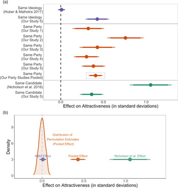
Figure 1 provides an overview of our results. (It focuses on the attractiveness outcome – the only one contained in all three studies.) As was mentioned earlier, Figure 1 shows the massive gap between the findings from Huber and Malhotra (Reference Huber and Malhotra.2017) and Nicholson et al. (Reference Nicholson, Coe, Emory and Song2016). The difference between the two is a staggering whole standard deviation.
The Effect Political Similarity on Evaluations of Attractiveness. [A] Comparison Across Studies. [B] Study Effects Relative to Permutation Estimates. Note: the effect of being in a similar group to the dating profile on perceived levels of attractiveness. Effects are plotted as points, with corresponding 90% (narrow line) and 95% (wider line) confidence intervals. Figure benchmarks our four estimates (middle) and a pooled estimate from a meta-analysis of these (highlighted with a box) to an ideology treatment from Huber and Malhotra (Reference Huber and Malhotra.2017) (on the top) and a candidate treatment from Nicholson et al. (Reference Nicholson, Coe, Emory and Song2016) (on the bottom). In our study 3, we use only those in the no-demand effects condition to parallel across the treatments. N’s from top to bottom: 9790 (unit of analysis: individual profile); 513 (individuals); 457 (individuals); 387 (individuals); 725 (individuals); 1786 (individuals); 3868 (individuals); 570 (individuals); and 1786 (individuals). We exactly replicate the models used in Huber and Malhotra (Reference Huber and Malhotra.2017) and Nicholson et al. (Reference Nicholson, Coe, Emory and Song2016), with the one exception of standardizing the outcome measures.

We start first by examining the effects of our party manipulation. Figure 1 shows that our partisanship treatments elicit a 0.408 standard deviation (95% CI: 0.33, 0.49) change when we pool our five experiments together. That is to say, being randomly assigned to a treatment of seeing a profile of someone who is the same political party as you has a modest effect on how attractive you rate them. These estimates are statistically significant at the 0.1% level and also distinct from random shuffles in permutation tests (see panel B). They are also quite different from what previous research has shown. Our pooled party effect is much smaller than Nicholson et al. (Reference Nicholson, Coe, Emory and Song2016)’s effect and much larger than that shown by Huber and Malhotra (Reference Huber and Malhotra.2017). Simply put, our results suggest that politics does not have a transformational effect on dating relationships but also does not have null effects.
This conclusion holds across reasonable design changes that could be explaining the chasm between previous results. First, Figure 1 shows that even when we use the exact same sampling frame as used by Nicholson et al (Reference Nicholson, Coe, Emory and Song2016) – i.e. the CCES (our Study 2) – their results are statistically (p < 0.05) and substantively (39%) larger than ours. Also, we should note that the attractiveness effect is uniquely large.
Second, our conclusion of a modest, not a null or transformational, effect holds when we make the treatments as similar as possible – testing simultaneously the effect of party, ideological, and candidate alignment (our Study 5). As can be seen, the reason for the differences between the Huber and Malhotra (Reference Huber and Malhotra.2017) and Nicholson et al. (Reference Nicholson, Coe, Emory and Song2016) studies does not appear to be because of a different individual identity being manipulated. In both cases, our treatments are substantively and significantly distinct from previous research. When we manipulate ideology, our effects are much larger than Huber and Malhotra (Reference Huber and Malhotra.2017)’s. When we manipulate candidate affiliation, Nicholson et al. (Reference Nicholson, Coe, Emory and Song2016)’s are still much larger. In fact, our ideological and candidate manipulations are much more similar in size – and not statistically distinct from – to our party treatments. Regardless of how you administer the treatment, politics has a modest – not a null or transformational – effect. (For all effects measured in Study 5, see Figure A4 in the Online Appendix.)
Third, our results suggest that the differences seen by Huber and Malhotra (Reference Huber and Malhotra.2017) and Nicholson et al. (Reference Nicholson, Coe, Emory and Song2016) are not due to timing. This may seem intuitive given that both of the earlier studies were conducted in 2012 (though perhaps in different months; the replication materials in the two papers are unclear on this point). However, our Experiment #5 affords us direct evidence that even when we equalize timing down to the exact same study fielded at the exact same time, we do not see effects similar to those observed by Huber and Malhotra (Reference Huber and Malhotra.2017) and Nicholson et al. (Reference Nicholson, Coe, Emory and Song2016). Why is this? Though it’s tough to know for sure, one explanation is that our results are consistent with partisan animus having grown since 2012 and Nicholson et al. (Reference Nicholson, Coe, Emory and Song2016)’s estimates being an outlier.
Fourth, the differences are not explained by how the treatment was administered – be it by the person in the profile or someone else (i.e. Study 4). Figure 1 also shows the effect of the potential partner being in an out-party on evaluations on measures of attractiveness. As can be seen, the treatment effect is still large in size, statistically significant, and not statistically or substantively distinct from our two other MTurk experiments. Simply changing the delivery mechanism still keeps us in the moderate effect domain.
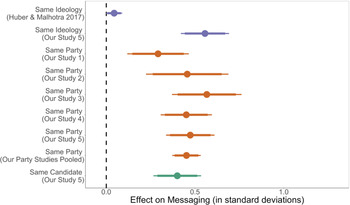
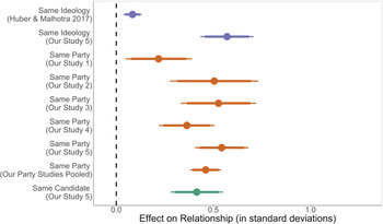
Fifth, our results of a modest, not null or transformational, effect holds when we look across different outcomes of dateability. As Figures 2 and 3 illustrate, the same part effect persists on our other measures that we explore. In addition to showing that our results hold across various outcome measures, our results suggest in total that partisan affect may be more than just disliking partisanship generally as some have suggested (e.g. Klar and Krupnikov Reference Klar and Krupnikov.2016, C.4; Klar et al. Reference Klar, Krupnikov and Ryan.2018; Klofstad et al. Reference Klofstad, McDermott and Hatemi.2012, Reference Klofstad, McDermott and Hatemi2013). If this were the case, we would expect to see dating profiles with any partisan information being penalized regardless of whether a person identifies with the same or a different party. Instead, we see a partisan asymmetry: individuals’ party plays a strong role in influencing how they evaluate people from the same or different parties.
Benchmarking to Previous Studies (Respond to Message). Note: figure displays the effect of being in a similar group to the dating profile on the respondent’s willingness to respond to a message. Effects are plotted as points, with corresponding 90% (narrow line) and 95% (wider line) confidence intervals. Figure benchmarks our three estimates (middle) from Studies 1, 2, 3, 4, and 5 and a pooled estimate from these to an ideology treatment from Huber and Malhotra (Reference Huber and Malhotra.2017) (on the top) and a same candidate treatment (from study 5). In our study 3, we use only those in the no-demand effects condition to parallel across the treatments. (Nicholson et al. Reference Nicholson, Coe, Emory and Song2016 is removed from this comparison as they only look at attractiveness.) N’s from top to bottom: 9790 (unit of analysis: individual profile – the rest are individual level); 1786, 513, 457, 387, 725, 1786, 3868, 1786.

Benchmarking to Previous Studies (Be in a Relationship). Note: figure displays the effect of being in a similar group to the dating profile on their willingness to see themselves in a long-term relationship with the person. Effects are plotted as points, with corresponding 90% (narrow line) and 95% (wider line) confidence intervals. Figure benchmarks our three estimates (middle) from Studies 1, 2, 3, 4, 5 and a pooled estimate from these to an ideology treatment from Huber and Malhotra (Reference Huber and Malhotra.2017) (on the top). In our study 3, we use only those in the no-demand effects condition to parallel across the treatments. (Nicholson et al. Reference Nicholson, Coe, Emory and Song2016 is removed from this comparison as they only look at attractiveness.) N’s from top to bottom: 9790 (unit of analysis: individual profile – the rest are individual level); 1786, 513, 457, 387, 725, 1786, 3868, 1786.

Finally, the differences in previous estimates are not explained by demand effects. Should demand effects exist, we would expect significant differences between those who were randomly assigned to be told the research question and those that were not. However, we find that there are no such differences. Our treatment effects are statistically indistinguishable and substantively the same, regardless of whether we tell the respondent our research question or not.
In short, regardless of the sampling framework used, the timing of the survey, the treatment used, how the treatment is administered, the outcomes one looks at, and demand effects are minimized, the results are the same – politics has modest, but not null or transformational, effects on relationship building.
Conclusion
This manuscript provides evidence that romantic relationships are influenced by politics, albeit simultaneously less and more than previous research has suggested. We have documented that this modest – but not null or transformational – effect is robust to many different experimental designs. These show that previous studies have given us an incomplete picture of how politics shapes the vitally important formation of relationships.
We note that there are important limitations to our analysis. First, we acknowledge that our experiment (like the experiments that preceded it) uses hypothetical profiles on a survey experiment and may not fully capture the effect of political affiliations on actual dating platforms such as Tinder or OKCupid. However, we (and our Institutional Review Boards) felt ethically restrained from creating false dating profiles on these platforms (what comes dangerously close to what some people call “catfishing”), as (among other reasons) under this design respondents would be unable to give their consent before engaging in the experiment. Further, our goal was to explore previous studies which also used hypothetical dating profiles. Given all this, using a survey experiment was the best available option. Second, like other experiments on politics and relationship formation, we have not tackled the extent to which partisan penalties are actually reflective of other intuited characteristics. While some experimental research on roommate selection suggests that when other individual characteristics are randomized politics that trumps other individual characteristics (Shafranek Reference ShafranekForthcoming), we cannot be certain this holds in relationship building. Future work would do well to explore the extent to which citizens use partisanship to intuit other characteristics of individuals and whether providing additional information affects the effects we have explored. Third, future work would do well to further consider the effect of the sample on estimates of partisanship on relationship building. While we have done so in some here (e.g. using MTurk and the CCES), future research would do well to consider effects in particular in online opt-in panels (e.g. Lucid). The extent to which our findings will differ from these samples will depend on the extent of treatment effect heterogeneity, where recent scholarship has shown to be fairly minimal across many survey experiments (e.g. Coppock, Leeper, and Mullinix Reference Coppock, Leeper and Mullinix.2018; Coppock and McClellan Reference Coppock and McClellan.2019). Finally, our outcomes don’t fully measure all aspects of a relationship, especially preferences that develop later in the dating process. While later-stage relationship building is important to measure, we purposefully designed our experiment to capture earlier inclinations that online daters are more likely to experience. The early part of relationship formation is especially important, given the potential for transformation and convergence once relationships have been well established (Iyengar et al. Reference Iyengar, Lelkes, Levendusky, Malhotra and Westwood.2019).
There is still much to be explored regarding affective polarization and romantic relationships. For example, there remains an important unanswered normative question in the literature on affective polarization about whether people should or should not be sorting by politics. While this question will inevitably come down to the values that one holds, future work would still do well to study the broader implications of partisan sorting for the well-being of individuals and society as a whole. While we have focused on the nature and the extent of bias, future work would do well to consider the consequences of such bias on the overall health of individuals, their relationships, and the communities in which they live.
Supplementary material
To view supplementary material for this article, please visit https://doi.org/10.1017/XPS.2020.21