
1. Introduction
Dispersive waves are ubiquitous in geophysical flows, such as flows in the atmosphere and world's oceans. These waves can spontaneously generate slowly evolving mean flows, enhance turbulent diffusivity of flows and are hypothesized to form an energy sink for balanced vortical flows (Bretherton Reference Bretherton1969; Francois et al. Reference Francois, Xia, Punzmann, Ramsden and Shats2014; Suanda et al. Reference Suanda, Feddersen, Spydell and Kumar2018; Xia et al. Reference Xia, Francois, Punzmann and Shats2019; Thomas & Daniel Reference Thomas and Daniel2020, Reference Thomas and Daniel2021; Thomas & Gupta Reference Thomas and Gupta2022). The balanced vortical mode in geophysical flows contain a major fraction of the total flow energy and mechanisms by which such mean flows can dissipate their energy is an unresolved question. Additionally, the irreversible modification of vortical flows by the presence of energetic dispersive waves is thought of as a means by which the lateral diffusivity of oceanic flows can be increased (Shcherbina et al. Reference Shcherbina2015). Turbulent exchanges between fast dispersive waves and slow vortical mean flows is therefore an active research area in geophysical fluid dynamics, with investigations focusing on potential mechanisms by which dispersive waves can form an energy sink for slow mean vortical flows and enhance local turbulent flow diffusivity.
Further to energy exchanges with slow mean flows and enhancing flow diffusivity, the turbulent dynamics of dispersive waves in geophysical flows are investigated to understand detailed mechanisms by which wave energy is transferred from large inviscid to small dissipative scales (Muller et al. Reference Muller, Arbic, Richman, Shriver, Kunze, Scott, Wallcraft and Zamudio2015; Dong, Bühler & Smith Reference Dong, Bühler and Smith2020; Pollmann Reference Pollmann2020). While vortical flows generically transfer energy upscale via an inverse energy flux, waves transfer energy downscale via a forward energy flux. This wave energy transfer from large to small scales is the predominant mechanism by which small scale mixing takes place in geophysical flows, especially in the world's oceans. Consequently, resolving mechanisms that trigger the forward flux of waves and identifying localized regions where waves dissipate are imperative for developing better parametrizations for large-scale atmosphere–ocean–climate models that are far from resolving the dynamics of a broad spectrum of fast dispersive waves (Garrett & Kunze Reference Garrett and Kunze2007; Alford et al. Reference Alford, MacKinnon, Simmons and Nash2016; Moum Reference Moum2021).
When compared with the above-mentioned interests and investigations into the energy exchanges of waves with vortical flows, wave-induced modification of flow diffusivity and the forward flux of waves, the least studied aspect of dispersive waves in geophysical flows is the upscale or inverse flux of waves. The inverse flux of waves is a non-trivial and counterintuitive feature that is specific to waves whose dispersion relationship does not allow resonant triads. Such wave systems, with deep water surface gravity waves and inertia-gravity waves in a shallow rotating fluid being popular examples, conserve wave action in addition to wave energy (Nazarenko Reference Nazarenko2011). The conservation of wave action and wave energy results in two kinds of turbulent transfers: a forward flux of wave energy and an inverse flux of wave action. The phenomenology is qualitatively analogous to that in two-dimensional hydrodynamic turbulence and quasi-geostrophic turbulence characterized by an upscale energy transfer and a downscale enstrophy transfer (Salmon Reference Salmon1978; Vallis Reference Vallis2006).
Theoretical calculations based on the weakly nonlinear wave turbulence formalism predicts the inverse flux of surface gravity waves (Zakharov, L'vov & Falkovich Reference Zakharov, L'vov and Falkovich1992), and in recent times a broad set of studies have examined this upscale wave transfer using direct numerical integration of the governing equations and laboratory experiments (Annenkov & Shrira Reference Annenkov and Shrira2006; Korotkevitch Reference Korotkevitch2008; Deike, Laroche & Falcon Reference Deike, Laroche and Falcon2011; Falcon et al. Reference Falcon, Michel, Prabhudesai, Cazaubiel, Berhanu, Mordant, Aumaitre and Bonnefoy2020). A key outcome of these and related studies is the appreciation that weakly nonlinear turbulent wave fields can exhibit significant departures from the idealized states assumed in wave turbulence formalism. Notably, non-Gaussian effects and intermittency in turbulent transfers are features that are generically seen in surface wave turbulence studies (Yokoyama Reference Yokoyama2004; Falcon, Fauve & Laroche Reference Falcon, Fauve and Laroche2007a; Falcon, Laroche & Fauve Reference Falcon, Laroche and Fauve2007b; Falcon et al. Reference Falcon, Aumaitre, Falcon, Laroche and Fauve2008; Korotkevitch Reference Korotkevitch2008; Falcon, Roux & Laroche Reference Falcon, Roux and Laroche2010). As a result, in addition to confirming some of the predictions of wave turbulence theory, these past studies have shed light on features that are missing in wave turbulence theory; providing theorists new opportunities to further investigate and improve the existing machinery of wave turbulence formalism.
Although the upscale transfer of waves is expected generically for dispersive waves with prohibited triadic interactions, as reflected in the above discussion, most of the upscale wave transfer investigations have focused on surface gravity waves and relatively little is known of inertia-gravity waves in the shallow fluid approximation, as applied to atmospheric and oceanic flows. The rotating shallow water equations (RSWE) capture the dynamics of a thin layer of rotating fluid and are the leading-order approximation for flows in the atmosphere and the ocean (Vallis Reference Vallis2006; Zeitlin Reference Zeitlin2018). As in the case of surface gravity waves, the inverse flux of inertia-gravity waves in RSWE has been predicted based on theoretical calculations (Falkovich Reference Falkovich1992; Falkovich & Medvedev Reference Falkovich and Medvedev1992; Glazman Reference Glazman1996). However, the calculations in Falkovich (Reference Falkovich1992) and Falkovich & Medvedev (Reference Falkovich and Medvedev1992) use classical wave turbulence theory that overlooks intrinsic features such as intermittency and non-Gaussian statistics, while the calculations in Glazman (Reference Glazman1996) includes higher-order wave interaction effects, an adhoc inclusion that does not have a formal asymptotic or a rigorous mathematical justification. Consequently, despite the upscale transfer of inertia-gravity waves being predicted via theoretical calculations three decades back, no confirmation for the phenomenon based on direct numerical integration of the governing equations exist to date.
One-dimensional RSWE is one of the simplest geophysical fluid dynamic models that captures multiple complex features of inertia-gravity waves and has been used consistently in the past to investigate wave-vortex dynamics, forward flux of waves and shock formation, dynamics of geophysical fronts, and the existence and stability of the slow manifold (Kuo & Polvani Reference Kuo and Polvani1997, Reference Kuo and Polvani1999; Zeitlin, Medvedev & Polougonven Reference Zeitlin, Medvedev and Polougonven2003; Bouchut, Le Sommer & Zeitlin Reference Bouchut, Le Sommer and Zeitlin2004). In this paper we investigate the inverse flux of waves and its intricate details in one-dimensional RSWE by direct numerical integration of the governing equations.
We specifically focus on one-dimensional RSWE in this study since the one-dimensional nature of the equations allows us to integrate the model for really long times maintaining high numerical accuracy. As will be seen below, long-time integration of the equations is crucial to the development of statistically steady upscale wave transfers. Additionally, it is noteworthy that significant advances in wave turbulence has been brought out by studying adhoc one-dimensional mathematical models such as the Majda–McLaughlin–Tabak model (Majda, McLaughlin & Tabak Reference Majda, McLaughlin and Tabak1997) and its generalizations (Cai et al. Reference Cai, Majda, McLaughlin and Tabak2001; Zakharov, Dias & Pushkarev Reference Zakharov, Dias and Pushkarev2004). Contrary to such adhoc models, one-dimensional RSWE is a physically relevant model that is often used as a work horse in geophysical fluid dynamic investigations. In this study we aim to explore features associated with the upscale transfer of waves in one-dimensional RSWE.
The plan for the paper is as follows: we present the equations and numerical integration details in § 2, upscale wave transfer results in § 3 and summarize our findings in § 4.
2. Equations, conservation laws, and numerical integration
The RSWE in one dimension are
 \begin{gather} \frac{\partial{u}}{\partial{t}} - fv + g \frac{\partial{h}}{\partial{x}} + u \frac{\partial{u}}{\partial{x}} = 0, \end{gather}
 \begin{gather}\frac{\partial{v}}{\partial{t}} + fu + u \frac{\partial{v}}{\partial{x}} = 0 , \end{gather}
 \begin{gather}\frac{\partial{h}}{\partial{t}} + H \frac{\partial{u}}{\partial{x}} + \frac{\partial{ (hu) }}{\partial{x}} = 0, \end{gather}
where  $(u, v)$ is the velocity vector,
 $h$ is the height deviation from the mean height
 $H$,
 $f$ is the rotation rate and
 $g$ is the acceleration due to gravity. We non-dimensionalize the above equations using
 \begin{gather} x \rightarrow L x, \quad t \rightarrow \left( \frac{L}{c_0} \right) t, \quad f \rightarrow \left( \frac{c_0}{L} \right) f, \quad (u, v) \rightarrow \left( \epsilon c_0 \right) (u, v), \quad h \rightarrow \left( \epsilon H \right) h. \end{gather}
In the above non-dimensionalization  $x$ coordinate was scaled by a length scale
 $L$ and
 $L/c_0$ was used to scale time, with
 $c_0 = \sqrt {g H}$ being the non-rotating gravity waves’ speed. The velocity was non-dimensionalized by a scale
 $U = \epsilon c_0$ while the height field fluctuations with respect to the mean were scaled by
 $\epsilon H$. Note that from the velocity scaling we have
 $\epsilon = U/c_0$. Therefore,
 $\epsilon$ is the Froude number, providing an estimate of how the flow velocity scales with the linear gravity wave speed. Throughout this work we will be based in the weakly nonlinear regime characterized by
 $\epsilon \ll 1$. Consequently, from the above scaling we have
 $h \ll H$ (in dimensional form), which means that the fluctuations in the height field are small compared with the mean height. Applying the scaling (2.2a–e) to (2.1) gives us the non-dimensional equations
 \begin{gather} \frac{\partial{u}}{\partial{t}} - f v + \frac{\partial{h}}{\partial{x}} + \epsilon u \frac{\partial{u}}{\partial{x}} = 0, \end{gather}
 \begin{gather}\frac{\partial{v}}{\partial{t}} + f u + \epsilon u \frac{\partial{v}}{\partial{x}} = 0, \end{gather}
 \begin{gather}\frac{\partial{h}}{\partial{t}} + \frac{\partial{u}}{\partial{x}} + \epsilon \frac{\partial{ (hu) }}{\partial{x}} = 0. \end{gather}
In the above equations,  $f$ is the non-dimensional rotation rate, based on the scaling described in (2.2a–e).
Inertia-gravity waves and the geostrophically balanced vortical mode form the linear modes of (2.3). In this work we discard the vortical mode and focus on the turbulent dynamics of inertia-gravity waves. The linear waves in (2.3) posses the dispersion relationship
 \begin{equation} \omega_k=\sqrt{f^2 + k^2}. \end{equation}
Total energy  $E^{\epsilon }$ is an integral conserved quantity of (2.3) and is given by the expression
 \begin{equation} E^{\epsilon} = \int_{x} \left \{ \tfrac{1}{2} (1 + \epsilon h) \left( u^2 + v^2 \right) + \tfrac{1}{2} h^2 \right \} {{\rm d} x}. \end{equation}
For  $\epsilon \ll 1$, the cubic energy expression (2.5) can be approximated by the quadratic energy expression
 \begin{equation} E = \int_{x} \left \{ \frac{1}{2} \left( u^2 + v^2 \right) + \frac{1}{2} h^2 \right \} {{\rm d} x} = \sum_{k} \left \{ \left\vert \hat {u}_k \right \vert^2 + \left \vert \hat{v}_k \right \vert^2 + \left \vert \hat{h}_k \right \vert^2 \right \} = \sum_{k} \hat{E}_k, \end{equation}
where  $(\hat {u}_k, \hat {v}_k, \hat {h}_k )$ is the Fourier transform of
 $(u, v, h)$. Although the exact energy expression (2.5) is cubic, in the weakly nonlinear regime with
 $\epsilon \ll 1$, the quadratic and cubic energies are indistinguishable. This was verified in all our numerical integrations and we refer the reader to the Appendix for a detailed confirmation.
The absence of resonant triads is a feature of the inertia-gravity waves’ dispersion relationship in (2.4) (see proof of this statement detailed in Babin, Mahalov & Nicolaenko Reference Babin, Mahalov and Nicolaenko1997 and Majda Reference Majda2002). The lack of resonant triads results in the conservation of wave action  $A$ given by (Falkovich Reference Falkovich1992; Falkovich & Medvedev Reference Falkovich and Medvedev1992; Glazman Reference Glazman1996)
 \begin{equation} A = \sum_k \hat{A}_k , \quad \hat{A}_k = \frac{ \hat{E}_k }{ \omega_k }. \end{equation}
It is important to note that the energy  $\hat {E}_k$ that appears in (2.7a,b) is the quadratic wave energy (2.6), excluding the vortical energy. Since in the present work we exclude the vortical mode, the wave fields are identical to the total fields and wave energy is identical to the total energy. The derivation of the conservation of wave action in (2.7a,b) requires writing the solution of the flow variables as the superposition of linear plane waves and then manipulating using the fact that linear waves have no potential vorticity. We omit further details of this derivation that is sketched in Falkovich (Reference Falkovich1992) and also refer the reader to chapter 8 of Nazarenko (Reference Nazarenko2011) for a more generic derivation applicable to arbitrary systems.
In the absence of the vortical mode, we therefore have conservation of wave energy and wave action. Although the exact energy conserved by RSWE is cubic, as mentioned above, the energy is very well approximated by the quadratic energy in the weakly nonlinear regime. The conservation of wave energy and wave action leads to two kinds of turbulent transfers: a downscale transfer of wave energy and an upscale transfer of wave action. Below we will use numerical integration of the equations to determine features associated with this upscale wave transfer.
2.1. Numerical integrations
To examine the upscale transfer of waves, we integrated (2.3) with  $\epsilon =0.1$ using a dealiased pseudospectral scheme in the periodic domain
 $x \in [0, 2 {\rm \pi}]$. Selected integrations were also performed in a domain twice the size to ensure that domain size did not affect results discussed below. The time integration was performed by using the implicit–explicit third-order Runge–Kutta method detailed in table 6 in Pareschi & Russo (Reference Pareschi and Russo2005). The nonlinear terms were treated explicitly while the dissipative terms described below were treated implicitly. We used the two-thirds dealiasing and denote the maximum wavenumber obtained after dealiasing by
 $k_{max}$. Waves were forced in a narrow band centred approximately around
 $k_{max}/3$. To ensure that the numerical results, especially statistics associated with the waves’ transfer in the inertial range, were insensitive to spatio-temporal resolution, we performed a series of numerical integrations with successively increasing resolutions. We first integrated the equations with
 $k_{max}=512$. At this spectral resolution the numerical integrations were carried out at successively smaller time steps until the solution was seen to be independent of the time step. Once converged in time, the spectral resolution was doubled and the numerical integrations were carried out again with decreasing time steps. This process was continued until it was confirmed that the resolution
 $k_{max} = 2048$ generated solutions that were insensitive to further increase in spectral resolution. Specifically, this resolution ensured that details of the turbulent transfer across the inertial range and the associated statistics described in the following section were robust and did not change on further increase in resolution. All the results presented in this paper were therefore generated with the spectral resolution
 $k_{max} = 2048$.
For the results presented in this paper with the spectral resolution of  $k_{max} = 2048$, waves were forced as white noise in a narrow wavenumber band centred at wavenumber 600 as
 $597 < k < 603$, with a stochastic forcing scheme, similar to that described in Alvelius (Reference Alvelius1999). To remove energy accumulating at small grid scales, we added hyperdissipative terms of the form
 $-\nu \partial ^{16}/\partial x^{16} (u, v, h)$ to the right-hand side of (2.3). To ensure that scales to the left of the forcing were free of viscous effects, we set the hyperviscosity
 $\nu$ to 0 for
 $k \leqslant 640$ and to
 $10^{-38}$ for
 $k > 640$. Linear drag terms of the form
 $-\gamma (u, v, h)$ were added to the right-hand side of (2.3) so that the drag formed an energy sink for wave energy reaching low wavenumbers. The drag coefficient
 $\gamma$ was set to 0 for
 $k>3$, ensuring that only a few low modes were effected by drag. Consequently, the inertial range that develops in the wavenumber interval
 $3 < k < 640$ was completely free of dissipative effects.
Numerical integrations were started from zero initial conditions, i.e. at  $t=0$ we set
 $u=v=h=0$, and the high wavenumber forcing was the only source of waves for the system. Numerical integrations beginning from a state of rest were seen to be required to go up to
 $t \sim 15\,000$ for the flow to form a broad spectrum of waves in a statistical steady state. The long-time forced-dissipative equilibrated state of the system was confirmed by monitoring energy and various statistical quantities described in the following section. Once the flow was seen to reach an equilibrated state, the equations were integrated for an interval
 $\Delta t = 50\,000$, this being the interval during which the averaging of statistical quantities given below were computed. A further increase in the averaging time interval was not seen to change the quantities by a noticeable margin, which is why we chose
 $\Delta t = 50\,000$ as the averaging interval.
3. Results
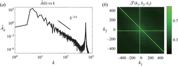
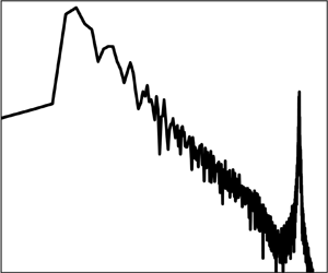
As mentioned earlier, in a turbulent flow composed of inertia-gravity waves, wave action is fluxed to larger scales. Consequently, the action flux moves waves forced at high wavenumbers to low wavenumbers or larger scales. For unit rotation rate  $f=1$, figure 1(a) shows the action spectrum of waves in forced-dissipative equilibrium. Since the waves’ dispersion relationship (2.4) prevents resonant triads, quartic resonances form the leading interaction. For a wavenumber quartet
 $(k, k_1, k_2, k_3)$, we have the resonance conditions
 \begin{equation} k = k_1 + k_2 + k_3 \end{equation}
and
 \begin{equation} \omega (k) ={\pm} \omega (k_1) \pm \omega (k_2) \pm \omega (k_3). \end{equation}
Note that every wavenumber, say  $k_1$ for example, can take positive and negative values, which is why we did not add
 $\pm$ in the wavenumber relationship in (3.1a). Solving the above resonance equations using the dispersion relationship (2.4) gives us
 $k_1 = -k_2$,
 $k_1=-k_3$ and
 $k_2=-k_3$ as the resonant curves. To examine the relevance of quartic resonances in the waves’ upscale transfer, we computed the tricoherence coefficient
 \begin{equation} \mathscr{T} (k_1, k_2, k_3) = \frac{ \vert \left \langle \hat{u}_k^* \hat{u}_{k_1} \hat{u}_{k_2} \hat{u}_{k_3} \right \rangle \vert }{ \langle \vert \hat{u}_k \vert \rangle \langle \vert \hat{u}_{k_1} \vert \rangle \langle \vert \hat{u}_{k_2} \vert \rangle \langle \vert \hat{u}_{k_3} \vert \rangle }, \end{equation}
where  $k= k_1 + k_2 + k_3$,
 $*$ denotes complex conjugate and
 $\langle \rangle$ denotes time averaging. The tricoherence coefficient,
 $0 \leqslant \mathscr {T} \leqslant 1$, is similar to the bicoherence coefficient used to examine triadic wave interactions (MacKinnon et al. Reference MacKinnon, Alford, Sun, Pinkel, Zhao and Klymak2013; Aubourg & Mordant Reference Aubourg and Mordant2015; Meyrand et al. Reference Meyrand, Kiyani, Gurcan and Galtier2018). We examined
 $\mathscr {T} (k_1, k_2, k_3)$ for a wide range of wavenumbers and an example visualization of the coefficient in the
 $k_1\unicode{x2013}k_2$ plane for
 $k_3=30$ is shown in figure 1(b). Note that the high correlation regions, which appear as bright green lines in the figure, correspond to resonant curves given by
 $k_1 =- k_2$,
 $k_1=-30$ and
 $k_2=-30$, as predicted by the resonant quartic solutions.
(a) Action spectrum for  $f=1$. Time-averaged spectral slope in the inertial range was seen to be
 $-3.6$. Panel (b) shows
 $\mathscr {T} (k_1, k_2, k_3)$ for
 $k_3=30$. The high correlation bright green lines are the resonant curves:
 $k_1=-k_3$,
 $k_2=-k_3$ and
 $k_1 = - k_2$.

Despite  $\mathscr {T} (k_1, k_2, k_3)$ being dominated by four wave resonances, there are signatures of near-resonant and non-resonant transfers. A reader staring carefully at figure 1(b) will notice that, although not as intense as the bright green lines, there are high correlation (greenish) regions located away from the bright lines; these regions being an indication of non-resonant transfers. Additionally, the exact resonance curves obtained by solving (3.1) are straight lines with zero thickness, whereas the lines in figure 1(b) have finite thickness and is a signature of near-resonant exchanges.
Overall, the behaviour seen in figure 1(b) was seen to be generic for wavenumbers throughout the system. Despite signatures of non-resonant and near-resonant transfers being persistent, high correlation regions in  $\mathscr {T} (k_1, k_2, k_3)$ generically coincide with exact four wave resonance curves, indicating that quartic resonant interactions are the predominant mechanism responsible for the upscale transfer of waves.
3.1. Non-local transfer of wave action
The above discussion of resonant modes indicates that wavenumbers of disparate lengths can interact and influence each other. For instance, a set of wavenumbers consisting of wavenumbers that are a decade apart,  $(k, k_1, k_2, k_3) = (30, 300, -300, 30)$, interact since this set lies on the resonant manifold
 $k_1=-k_2$. In general, the resonant manifolds
 $k_1 =-k_2$,
 $k_1=-k_3$ and
 $k_2=-k_3$ are all composed of a broad set of non-local wavenumbers, indicating that the upscale transfer of waves in RSWE involves the interaction of non-local modes.
Of course, non-local wavenumbers being involved in the turbulent transfer term does not necessarily imply that the transfer itself is non-local. For instance, as is the case in three-dimensional homogeneous isotropic turbulence (3-D HIT), the turbulent transfer can be local although non-local modes participate in the transfer. To place these ideas on a firm foundation, especially for the sake of readers unfamiliar with local and non-local turbulent transfers, we will briefly visit these well established notions in 3-D HIT before dwelling into the locality of transfers in RSWE.
In 3-D HIT energy is fluxed downscale via triadic interactions. The energy equation in spectral space reads
 \begin{equation} \frac{\partial{\hat{E}_k}}{\partial{t}} = \sum_{k_1} \sum_{k_2} S_E (k \vert k_1, k_2) = \sum_{k_1} T_E (k \vert k_1) = R_E (k). \end{equation}
In the above equation,  $S_E (k \vert k_1, k_2)$ is the triadic nonlinear term in spectral space responsible for all energy transfer between wavenumbers
 $\boldsymbol {k}_1$,
 $\boldsymbol {k}_2$ and
 $\boldsymbol {k}$ subject to the triadic constraint
 $\boldsymbol {k}=\boldsymbol {k}_1+ \boldsymbol {k}_2$. Summing
 $S_E (k \vert k_1, k_2)$ over
 $k_2$ gives us the transfer function
 $T_E (k \vert k_1)$, which captures transfers between wavenumbers
 $k$ and
 $k_1$. Finally, summing over
 $k_1$ gives us the net energy transfer at a specific wavenumber,
 $R_E(k)$.
Locality of transfers in turbulent flows is quantified based on  $T_E(k \vert k_1)$ in (3.3), which captures the transfers between wavenumbers
 $k$ and
 $k_1$. Since
 $S_E(k \vert k_1, k_2)$ was summed over
 $k_2$ to obtain
 $T_E(k \vert k_1)$, it is clear that non-local triads contribute towards transfer of energy across scales. For instance, the lengths of wavenumbers
 $k$ and
 $k_1$ can be comparable, while
 $k_2$ can be of really small length resulting in
 $k_2 \ll k \sim k_1$. Such widely separated or non-local wavenumbers can affect the transfer. Although non-local wavenumbers participate in the transfer, conventionally in hydrodynamic turbulence a transfer is identified as local if most of the transfer term
 $T_E(k \vert k_1)$ is concentrated on wavenumbers
 $k \sim k_1$. This means that the transfer at a specific wavenumber
 $k$ is due to wavenumbers
 $k_1$ in the neighbourhood of
 $k$ such that
 $k/k_1 \sim 1$. On the other hand, if wavenumbers
 $k_1$ significantly away from
 $k$ such that
 $k/k_1 \gg 1$ or
 $k/k_1 \ll 1$ contribute towards the transfer at wavenumber
 $k$, it is termed a non-local transfer (Brasseur & Wei Reference Brasseur and Wei1994; Lesieur Reference Lesieur2008).
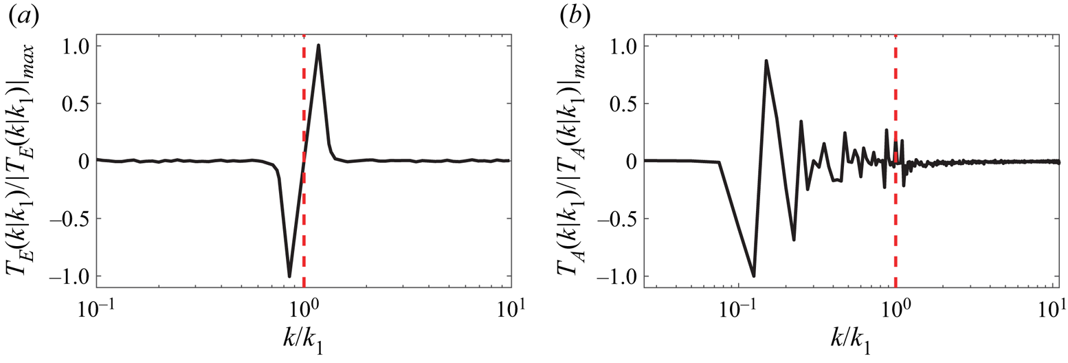
A broad set of studies focusing on 3-D HIT have revealed that although non-local wavenumbers play a role in the transfer, the energy transfer from large to small scales is local (Domaradzki & Rogallo Reference Domaradzki and Rogallo1990; Yeung & Brasseur Reference Yeung and Brasseur1991; Ohkitani & Kida Reference Ohkitani and Kida1992; Waleffe Reference Waleffe1992; Zhou Reference Zhou1993; Brasseur & Wei Reference Brasseur and Wei1994; Domaradzki & Carati Reference Domaradzki and Carati2007; Eyink & Aluie Reference Eyink and Aluie2009; Cardesa, Vela-Martin & Jimenez Reference Cardesa, Vela-Martin and Jimenez2017). Figure 2(a) shows an example plot of time averaged  $T_E(k \vert k_1)$ normalized by the maximum absolute value of the transfer term from a
 $2048^3$ resolution 3-D HIT numerical integration with
 $k$ being chosen to be in the middle of the inertial range. The numerical set-up was similar to that used in Thomas & Daniel (Reference Thomas and Daniel2020, Reference Thomas and Daniel2021), except that the incompressible Navier–Stokes equations were integrated instead of the Boussinesq equations integrated in Thomas & Daniel (Reference Thomas and Daniel2020, Reference Thomas and Daniel2021). The flow was stochastically forced at low wavenumbers and was dissipated at small scales by hyperdissipation. We skip further technical details here primarily since figure 2(a) is a popular result that has been persistently observed in a wide range of studies exploring the locality of turbulent transfers in 3-D HIT (see similar figures in Domaradzki & Rogallo (Reference Domaradzki and Rogallo1990) and Yeung & Brasseur (Reference Yeung and Brasseur1991) for example). For a reader unfamiliar with the locality of transfers in HIT, it is crucial to note that the transfer function
 $T(k \vert k_1)$ is localized around
 $k \sim k_1$. Observe how the function is negative for
 $k< k_1$ and positive for
 $k>k_1$, implying that energy is being transferred locally from left to right. The energy transfer at a specific wavenumber
 $k$ is therefore exclusively due to wavenumbers
 $k_1$ in the neighbourhood of
 $k$. Figure 2(a) therefore summarizes a well-established feature of the turbulent energy cascade in 3-D HIT: despite non-local wavenumbers being involved in the transfer term, the turbulent downscale transfer of energy is local.
Transfer terms normalized by their absolute maximum for (a) 3-D HIT and (b) RSWE. The transfer terms were time averaged to remove fast-in-time high frequency fluctuations.

Although 3-D HIT has no straightforward connections to the present study focusing on RSWE, the above discussion of locality of transfers in 3-D HIT was to introduce an unfamiliar reader to key technical details of the locality of turbulent transfers. Given the understanding summarized in the above passages on the locality of transfers, we will now examine the locality of transfers in RSWE. To get a handle on wave action transfer in RSWE, we take the Fourier transform of (2.3) and manipulate to form the wave action equation in spectral space as
 \begin{equation} \frac{\partial{ \hat{A}_k}}{\partial{t}} = \sum_{k_1} T_A (k \vert k_1). \end{equation}
Above,  $T_A (k \vert k_1)$ captures action transfer between wavenumbers
 $k$ and
 $k_1$ and summing over
 $k_1$ gives us the net action transfer at a specific wavenumber
 $k$. Figure 2(b) shows the time-averaged transfer function
 $T_A (k \vert k_1)$ normalized by the absolute maximum of the transfer term for RSWE with
 $k=50$, a wavenumber in the middle of the inertial range as can be seen from figure 1(a). Observe that the transfer term is highly non-local: the transfer has little contribution from the local neighbourhood of
 $k \sim k_1$ and the major fraction of the contribution to the transfer term is from wavenumbers
 $k_1$ located significantly away from
 $k$. Although the quantitative details in figure 2(b) are for a specific wavenumber
 $k=50$, the qualitative nature of the figure was seen to be generic for wavenumbers across the inertial range, i.e. extremely disparate wavenumbers
 $k_1$ are responsible for the transfer at a wavenumber
 $k$. The upscale transfer of inertia-gravity waves is therefore a non-local turbulent transfer involving the action transfer between extremely disparate scales or wavenumbers. Interestingly, examples of highly non-local transfers in dispersive wave turbulence have been observed in the past (see, for example, discussions in Cai et al. Reference Cai, Majda, McLaughlin and Tabak1999), non-local transfers being a feature that distinguishes scale-local strongly nonlinear transfers in 3-D HIT from resonance-dominated transfers in weakly nonlinear wave turbulence such as the one explored in our present study.
3.2. Intermittency in upscale transfers
Our findings so far point out that upscale wave transfers based on resonant four wave interactions is robustly seen in RSWE, as predicted by wave turbulence theory. Despite observing the upscale transfers as per the theoretical prediction, we found features of the flow such as intermittency and non-Gaussian statistics, indicating departures from assumptions used in classical wave turbulence theory. Intermittency of turbulent transfers is a persistent feature seen in turbulent wavy flows (Falcon et al. Reference Falcon, Fauve and Laroche2007a,Reference Falcon, Laroche and Fauveb, Reference Falcon, Aumaitre, Falcon, Laroche and Fauve2008, Reference Falcon, Roux and Laroche2010; Falcon & Mordant Reference Falcon and Mordant2022) and we found strong features of intermittency in our solutions and transfer across scales. On tracking different variables associated with the turbulent transfer, the action flux was seen to be an obvious indicator of intermittent transfers. Summing (3.4) from the lowest wavenumber to an arbitrary wavenumber gives us the time evolution equation of wave action contained in the wavenumber band  $[0, k]$ as
 \begin{equation} \frac{{\rm d}{ }}{{\rm d}{t}} \left( \sum_{n=0}^{n=k} \hat{A}_n \right) = \varPi_k, \end{equation}
where  $\varPi _k$ is the flux of wave action. Since action is being transferred from smaller scales to larger scales, on average the flux
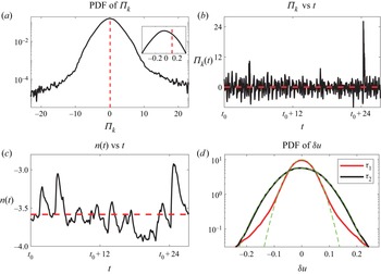
 $\varPi _k$ should be positive. Figure 3(a) shows the probability density function (PDF) of flux for an example wavenumber
 $k=50$, with the dashed red line showing the mean of the PDF. Note that the flux PDF is almost symmetric, with a slight skewness to the right. The mean of the action flux is positive, indicating that waves are on average getting transferred upscale. To highlight a specific detail of the transfer, figure 3(b) shows a short-time series of the action flux. Observe that the flux oscillates between positive and negative values with intermittent positive jumps: a notable positive jump is seen at
 $t=24.5$ in figure 3(b). The upscale transfer of waves is associated with such localized-in-time positive jumps in the action flux, these intermittent events being the cause of the slightly skewed PDF with a positive mean shown in figure 3(a). Although these details correspond to
 $k=50$, the intermittency of flux was observed generically for wavenumbers in the inertial range.
Panel (a) shows the PDF of action flux  $\varPi _k$ for
 $k=50$ while the inset shows a smaller part of the PDF. The mean of the PDF is shown by the dashed red vertical line. The PDF has skewness 0.19 and kurtosis 5.6. Panel (b) shows a short-time series of the action flux
 $\varPi _k$ for
 $k=50$ and
 $t_0$ is a reference time instant. The mean of the time series is indicated by the dashed red horizontal line. Observe that the flux time series shows a strong positive jump at
 $t=t_0+24.5$. Panel (c) shows a short-time series of the slope of the inertial range. Note that the slope takes up a high value, i.e. becomes shallower, following the positive burst in flux at
 $t=t_0+24.5$. The mean slope,
 $n=-3.6$, is indicated by the horizontal dashed red line and is marked by the straight black line in figure 1(a). Panel (d) shows the PDF of the velocity increment
 $\delta u = u(t+\tau ) - u(t)$ for
 $\tau _1=0.2$ and
 $\tau _2=5$.

The intermittent upscale transfers described above were seen to directly affect the inertial range of waves. Specifically, the slope of the waves’ spectrum was seen to change with time, with the spectrum becoming shallower following the positive bursts in flux. Figure 3(c) shows the slope of the spectrum,  $n(t)$, as a function of time in the same time interval as figure 3(b). The time-averaged slope of the spectrum is
 $-3.6$ and is marked by the dashed red line, this being the slope marked in figure 1(a). On comparing figures 3(b) and 3(c), it can be seen that the positive jump in flux at
 $t=24.5$ is followed by the highest slope in the time interval shown. On examining different windows of time series of the waves’ spectral dynamics, this was seen to be a generic feature: intermittent positive jumps in flux are followed by the waves’ spectrum becoming shallower, indicating an energization of waves across scales in the waves’ spectrum.
The intermittent dynamics of waves in spectral space described above corresponds to similar changes in physical space. A common tool to visualize intermittency is to track the changes in the PDF of velocity differences  $\delta u (\tau ) = u(t+\tau ) - u(t)$ (Frisch Reference Frisch1995). Specifically, PDFs of velocity increments,
 $\delta u$, deform with time lag
 $\tau$. At short-time lags,
 $\delta u$ has fat tails compared with a Gaussian distribution, while at longer
 $\tau$ the PDF approaches a Gaussian distribution. This behaviour of PDFs of increments in velocity deforming with time lag is a signature of intermittency and has been reported multiple times in surface wave turbulent flows (Falcon et al. Reference Falcon, Laroche and Fauve2007b, Reference Falcon, Roux and Laroche2010). Figure 3(d) shows the PDFs of the
 $\delta u$ for
 $\tau =0.2$ and
 $\tau =5$. The deformation of the PDF from a fat tailed distribution at lower
 $\tau$ to approaching a Gaussian distribution for larger
 $\tau$ is a direct reflection of intermittent turbulent transfers.
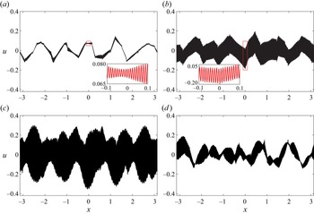
Tracking the flux and the inertial range behaviour of waves, we found that the intermittent events started at small scales and then propagated to larger scales. This information is reflected in figure 3(d), which indicates that intermittency is highest at small scales and lowest at large scales. The intermittent positive bursts in flux transfers waves upscale, eventually affecting domain-scale waves. On carefully monitoring the wave fields over time, we consistently observed that the intermittent positive jumps in flux were followed by higher energy level domain-scale waves. An illustration of this is shown in figure 4, the four panels corresponding to four different times in the time interval shown in figures 3(b) and 3(c). Note that the wave field's amplitude is highest in figure 4(c), which corresponds to the flux burst at  $t=t_0+24.5$ seen in figure 3(b). Away from the flux burst point, the amplitude of the wave field is relatively small, as can be seen in panels 4(a), 4(b) and 4(d). On examining the physical structure of waves across long-time intervals, we observed that the intermittent positive burst in the waves’ flux goes hand in hand with an amplification of the waves’ strength in physical space, i.e. high wave amplitudes were in general positively correlated with flux bursts.
The physical structure of  $u$ at four different times in the neighbourhood of the positive jump in flux at
 $t=t_0+24.5$ seen in figure 3(b). Specifically, u is shown at (a)
 $t=t_0+23.9$, (b)
 $t=t_0+24.2$, (c)
 $t=t_0+24.5$, (d)
 $t=t_0+24.7$. The insets in panels (a,b) show a zoomed-in view of the red rectangular regions in the main figures. The highest amplitude waves, seen in panel (c) above, correspond to the flux burst at
 $t=t_0+24.5$ in figure 3(b).

3.3. Departure from Gaussian statistics
Gaussian statistics for the flow fields and a random distribution of wave phases are typical assumptions used in wave turbulence theory (Zakharov et al. Reference Zakharov, L'vov and Falkovich1992; Nazarenko Reference Nazarenko2011). Therefore, a random uncorrelated distribution for the phases  $\text {arg}(\hat {u}_k), \text {arg}(\hat {v}_k), \text {arg}(\hat {h}_k)$ is expected in wave turbulent flows. We examined the statistics of the flow variables from our solutions and figure 5(a) shows the distribution of the phase,
 $\text {arg}(\hat {u}_k) \in [-{\rm \pi}, {\rm \pi}]$, for three wavenumbers,
 $(k_1, k_2, k_3)=(10, 50, 300)$. The phases were averaged over a long interval such that the distribution saturated to that shown in the figure. As seen in the figure, the phases are less uniform at low wavenumbers and approach a uniform distribution at high
 $k$. A similar behaviour is seen for the PDF of
 ${\rm Re} (\hat {u}_k)$, the real part of
 $\hat {u}_k$, shown in figure 5(b). Observe that the lowest wavenumber shows a bimodal distribution that transitions gradually into a Gaussian distribution for the highest wavenumber.
(a) The PDF of phases of  $\hat {u}_k$ for three different wavenumbers
 $(k_1, k_2, k_3)=(10, 50, 300)$. (b) The PDF of the real part of
 $\hat {u}_k$ for the same three wavenumbers. A Gaussian curve is shown by a dashed green line for reference.

It is intriguing that although intermittency was seen to propagate from small scales to large scales, as discussed in § 3.2, the departure of wave phase and amplitude from idealized Gaussian distribution that is typically assumed in wave turbulence theory is highest at large scales. Furthermore, it is noteworthy that large scales carrying most of the energy departing from Gaussian distribution is a feature that has been observed in multiple past studies, especially studies focusing on waves undergoing a forward flux (Yokoyama Reference Yokoyama2004; Chibbaro & Josserand Reference Chibbaro and Josserand2016). Given these past results, we speculate that our finding of the departure from Gaussian statistics at large scales might not be specific to the upscale transfer of waves. The large scales carrying most of the total energy in the system departing from idealized Gaussian assumptions could be a more generic result applicable to arbitrary turbulent wavy systems, independent of whether the waves undergo forward or inverse flux.
3.4. Effect of increasing rotation rate
On increasing the rotation rate we observed that upscale transfers were weakened and it took a much longer time to form broad spectrum waves in forced-dissipative equilibrium. As follows from the dispersion relationship (2.4), for a fixed wavenumber, the wave frequency increases with  $f$ and the group velocity of waves
 $\boldsymbol {c}_g = \boldsymbol {k}/\sqrt {f^2 + k^2}$ decreases with increasing
 $f$, making propagation of wave packets slower. Furthermore, increasing
 $f$ reduces the scale-specific Rossby number,
 $Ro_k = k U_k/f$, where
 $U_k$ is the flow velocity magnitude at wavenumber
 $k$. The reduction in Rossby number and wave group velocity weakens the nonlinear interactions, making turbulent transfers slow and inefficient at higher rotation rates. A qualitatively similar effect was seen in Farge & Sadourny (Reference Farge and Sadourny1989) while investigating wave-vortex dynamics in two-dimensional RSWE. Farge & Sadourny found that high rotation rates led to a ‘freezing’ of the turbulent transfers in their relatively short-time interval numerical integrations. In our investigation, due to weakened upscale transfers, we had to numerically integrate the equations for much longer times. With weakened nonlinear interactions and slower turbulent transfers, we found the wave energy levels to slightly increase at an intermediate wavenumber, rather than the lowest wavenumbers, resulting in slightly steeper wave spectra at higher
 $f$.
The features mentioned above can be seen in the waves’ spectra for different  $f$ in figure 6: observe that the energy content at low wavenumbers,
 $k \lesssim 15$, is less for
 $f=4$ and
 $f=2$ when compared with the
 $f=1$ case, and the spectra are slightly steeper at higher
 $f$. Apart from reduced upscale transfers and other minor quantitative changes, all the qualitative features described earlier for
 $f=1$, i.e. resonant quartics playing the major role in upscale transfers, the non-local nature of the transfer, intermittency of the transfer observed in the inertial range and in the physical structure of the waves, and low wavenumbers departing the most from idealized Gaussian assumptions, were seen to be similar at higher rotation rates. We therefore omit further figures on turbulent transfers at high rotation rates and end on the note that upscale transfers are retarded on increasing the rotation rate.
Action spectra for different  $f$. The black curve is the same spectrum shown in figure 1. Note that the energy content at low wavenumbers decreases at higher
 $f$.

3.5. Comparison with predictions based on wave turbulence theory
As discussed earlier, wave turbulence theory has been applied to RSWE to obtain predictions for the turbulent spectra corresponding to the waves’ upscale transfer. Based on theoretical calculations, Falkovich (Reference Falkovich1992) and Falkovich & Medvedev (Reference Falkovich and Medvedev1992) found that the waves’ action spectrum was between  $k^{-13/3} \approx k^{-4.3}$ and
 $k^{-8/3} \approx k^{-2.7}$ for different limits of rotation and dispersion. Following this, Glazman (Reference Glazman1996) extended the theoretical calculations by including higher-order wave interactions and obtained slightly refined estimates for the waves’ spectrum. It is noteworthy that all the spectra we obtained by numerical integration of the governing equations lie between
 $k^{-4.3}$ and
 $k^{-2.7}$ (see figure 6), which is the range of spectra predicted based on wave turbulence theoretical calculations by Falkovich (Reference Falkovich1992) and Falkovich & Medvedev (Reference Falkovich and Medvedev1992).
Despite the waves’ spectra we obtained being within the interval predicted by previous theoretical estimates, multiple caveats must be emphasized here. In wave turbulence theoretical formalism, the waves’ spectrum emerges as an equilibrium solution, that is, the exponent  $n$ of the spectrum
 $k^{-n}$ is a fixed number. However, as explained earlier, the waves’ upscale transfers are intermittent and not steady, leading to a waves’ spectrum that fluctuates significantly over time (recall figure 3c). Additionally, Gaussian statistics and random phases for wave fields are central assumptions in wave turbulence theory, these conditions also not being satisfied by the solution of the equations we found (recall figure 5). To obtain improved estimates for the waves’ spectrum, Glazman (Reference Glazman1996) included higher-order wave interaction terms and assumed the locality of transfers in spectral space, a feature that was seen to be violated in upscale transfers in RSWE, as explained in connection to figure 2.
The above discussion brings out the challenges in comparing theoretical wave turbulence based predictions with numerical results obtained in the present work. Much of the idealized assumptions used in wave turbulence theory are not satisfied by the solutions of the governing equations we obtained via direct numerical integrations. Not surprisingly, similar departures have been reported in numerical and laboratory experiments exploring turbulent dynamics of waves in different set-ups (Yokoyama Reference Yokoyama2004; Falcon et al. Reference Falcon, Fauve and Laroche2007a,Reference Falcon, Laroche and Fauveb; Korotkevitch Reference Korotkevitch2008; Falcon et al. Reference Falcon, Aumaitre, Falcon, Laroche and Fauve2008, Reference Falcon, Roux and Laroche2010; Chibbaro & Josserand Reference Chibbaro and Josserand2016). Our results therefore add to the growing list of evidence of wave turbulence theoretical predictions departing from numerical and experimental results on weakly nonlinear turbulent wave-dominated flows. These findings in general stress the need to improve the theoretical foundations of wave turbulence theory, so as to obtain better theoretical predictions that align with numerical and experimental results.
4. Summary and perspectives
In this paper we explored the upscale transfer of inertia-gravity waves in one-dimensional RSWE. The dispersion relationship of inertia-gravity waves in RSWE prohibits resonant triads, leading to a second integral conserved quantity in addition to energy: wave action. Consequently, in a turbulent flow consisting of inertia-gravity waves, wave energy is transferred to small scales while wave action gets transferred to larger scales. Although theoretical calculations based on wave turbulence theory have predicted the possibility of upscale wave transfers three decades back, no study has confirmed the phenomenon by integrating the governing equations. The lack of an investigation exploring the details of the waves’ upscale turbulent transfer inspired our present work, where we used direct numerical integration of the equations to study the upscale transfer of waves.
Our study revealed that resonant four wave interactions were primarily responsible for the waves’ upscale transfer. Non-local wavenumbers were involved in the turbulent transfer and the transfer itself was non-local, i.e. wave action was exchanged between extremely disparate scales. Additionally, the turbulent transfer was not continuous in time, rather upscale transfers took place via localized-in-time bursts of the action flux that moved waves on average to larger scales. These intermittent bursts in action flux went hand in hand with the shallower waves’ spectra and energetic high amplitude wave fields in physical space. The intermittency of upscale wave transfers were therefore noticeable in spectral space and physical space. Finally, the statistics of the wave field were seen to depart from Gaussian at larger scales, while smaller scales exhibited Gaussian behaviour. This shows a departure from typical assumptions used in wave turbulence theory, where the wave phases, for example, are assumed to be random and uncorrelated with Gaussian dynamics.
Contrary to vortical turbulent dynamics that requires at least two physical dimensions, wave turbulence can be realized in a single dimension. This attractive feature has inspired the development and integration of multiple one-dimensional mathematical models exploring turbulent dynamics of a broad spectrum of waves (Majda et al. Reference Majda, McLaughlin and Tabak1997; Cai et al. Reference Cai, Majda, McLaughlin and Tabak2001; Zakharov et al. Reference Zakharov, Dias and Pushkarev2004). Similar inspirations have led to studies exploring wave turbulent-like dynamics in one-dimensional Burgers equation (see discussions and references in Murray & Bustamante Reference Murray and Bustamante2018). The key here is that long-time high accuracy numerical integration is possible for one-dimensional models with affordable computational resources, allowing us to dwell into details of turbulent transfers that are not straightforward with higher-dimensional models. On a relative comparison, one-dimensional RSWE is a more realistic physical model than previously mentioned adhoc toy models and is a popular work horse in the geophysical fluid dynamics community. With the forward flux and multiple related dynamics of this model being explored in the past, our findings point out that the model also captures the rich non-trivial dynamics associated with the inverse flux of waves. Consequently, one-dimensional RSWE could be used as a slightly more realistic model than pre-existing adhoc models for future studies focusing on aspects related to the upscale transfer of dispersive waves.
Despite capturing the inverse flux of inertia-gravity waves, a notable feature observed in the present study was that the upscale transfers were generically slow, with  $t \sim O(10\,000)$ being the typical time scale to obtain a broad spectrum of waves in forced-dissipative equilibrium. Figure 7 shows, for example, the different stages of the waves’ spectra until it reaches an equilibrated state. Given the slow nature of the process, it is unclear how noticeable the upscale transfer of waves would be in realistic atmospheric and oceanic flows where many other processes operate on much faster time scales. However, although the waves’ spectrum takes a long time to reach equilibrium, intermittent and bursty upscale transfers detailed with figures 3 and 4 were seen during the intermediate stages shown in figure 7, before reaching equilibrium. Therefore, even on relatively short-time scales, wave activity at small scales can intermittently propagate to larger scales and accumulate at the inertial frequency, this being the ubiquitous low frequency peak in the oceanic wave spectrum (Garrett Reference Garrett2001; Alford et al. Reference Alford, MacKinnon, Simmons and Nash2016). Direct forcing by wind and spontaneous emission by vortical flows are considered to be the prominent mechanisms responsible for the inertial peak (D'Asaro Reference D'Asaro1985; Vanneste Reference Vanneste2013). Notably, there is no obvious explanation for near-inertial waves in regions with negligible wind forcing and vortical flow. Therefore, the inverse flux of inertia-gravity waves could play a role in energizing an inertial frequency peak in such regions, despite the slow nature of the waves’ upscale transfers.
Action spectra for  $f=1$ case at three different times. The broad spectrum of waves reaches an equilibrated state around
 $t=15\,000$.

Turbulent transfers in coastal oceanographic regions is another area where upscale wave transfers could have potential relevance. Multiple observations have indicated upscale transfers in shallow oceanographic regions near the coast (Soh & Kim Reference Soh and Kim2018; Yoo, Kim & Kim Reference Yoo, Kim and Kim2018; Elgar & Raubenheimer Reference Elgar and Raubenheimer2020). However, quite often the inverse flux is attributed to the vortical mode alone and the waves’ contribution is not critically evaluated. In other words, although upscale transfers are observed in coastal areas, there has been no dedicated efforts to separate the transfers due to waves alone from the vortical transfers. As mentioned earlier, given the slow nature of the upscale transfer of waves, further studies in realistic settings are needed to compare the relative rates of the upscale transfer of vortices and waves so as to examine whether the inverse flux of waves in coastal regions can form a non-negligible contribution to the net inverse flux of the flow.
Finally, the results of the present work point towards interesting ramifications for long term dynamics of RSWE, specifically in two dimensions. Given that our study confirms the inverse flux of inertia-gravity waves in one dimension, we anticipate the same phenomenon in two dimensions. Furthermore, the vortical mode that was ignored in the present study evolves and fluxes energy upscale in two dimensions. This means that both waves and the vortical mode can exhibit upscale transfers in two dimensions, challenging a well-established paradigm in geophysical fluid dynamics. In geophysical flows waves typically dissipate at small viscous scales due to downscale energy transfer while the vortical mode transfers energy upscale and undergoes negligible dissipation. As a result of waves disappearing from the system by small-scale dissipation, the long-time state of geophysical flows is assumed to be composed primarily of the vortical mode and negligible waves, this process being an example of turbulent geostrophic adjustment (Bartello Reference Bartello1995; Reznik Reference Reznik2015).
In light of the present study, it is natural to speculate that the upscale transfer of waves would result in a non-negligible amount of waves at large scales, along with the vortical mode. Consequently, contrary to the conventional hypothesis based on geostrophic adjustment, the long-time limit of RSWE in two dimensions could be a mixture of fast inertia-gravity waves alongside slowly evolving vortices. Surprisingly, almost four decades back Warn (Reference Warn1986) used equilibrium statistical mechanics machinery to predict that the long-time state of RSWE would be rich with fast inertia-gravity waves (also see the generalization of Warn's result by Renaud, Venaille & Bouchet Reference Renaud, Venaille and Bouchet2016). This unusual result of Warn and the details of the process remain untested to date, primarily due to the lack of extremely long-time numerical integration results of two-dimensional RSWE with waves and vortical modes. Past studies that have numerically integrated two-dimensional RSWE have focused primarily on the dynamics of the vortical mode, wave-vortex interactions on short-time scales and the forward flux of waves and shock formation (Farge & Sadourny Reference Farge and Sadourny1989; Polvani et al. Reference Polvani, McWilliams, Spall and Ford1994; Yuan & Hamilton Reference Yuan and Hamilton1994; Remmel & Smith Reference Remmel and Smith2009; Ward & Dewar Reference Ward and Dewar2010; Lahaye & Zeitlin Reference Lahaye and Zeitlin2012), contributing to the lack of an understanding of the long-time state of RSWE. Given the upscale wave transfers in RSWE, although specific details might differ, it is tempting to think that Warn's conclusion might have some significance in the long-time limit of RSWE.
Of course, investigating the above-mentioned realistic processes and the long-time limit of RSWE mentioned in the previous paragraph will require high-resolution long-time direct numerical integration of the two-dimensional RSWE by including the vortical mode. As mentioned earlier, in the present study the one-dimensional nature of the equations allowed us to integrate the equations for really long-time scales with high precision numerical accuracy. A typical time scale for obtaining forced-dissipative equilibrium flows and collecting all the relevant statistical quantities in our one-dimensional study was  $t \sim O(50\,000)$ and it is extremely challenging to integrate the two-dimensional RSWE for such long times. Consequently, decoding turbulent upscale transfers in two-dimensional RSWE remains to be an exceptionally challenging undertaking. In conclusion, although many different facets of RSWE have been explored in the past (Zeitlin Reference Zeitlin2018), the turbulent long-time state of RSWE still remains an open question that requires a detailed investigation.
Funding
J.T. thanks the Science & Engineering Research Board (SERB) of India for financial support through the project SRG/2022/001071.
Declaration of interests
The authors report no conflict of interest.
Appendix. Confirmation that linear waves dominate the flow
All the numerical integrations of (2.3) with  $\epsilon \ll 1$ were performed with wave forcing alone, excluding the vortical mode. Here we present details of the flow structure to confirm that the flow was dominated by linear inertia-gravity waves alone.
As mentioned in § 2, the quadratic and cubic energies given by (2.5) and (2.6) are indistinguishable in the weakly nonlinear regime. In all our numerical integrations, the quadratic energy  $E$ was seen to approximate the cubic energy
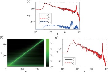
 $E^\epsilon$ very well. Furthermore, the quadratic and cubic energies were seen to agree well pointwise in physical and spectral space. A specific example is shown in figure 8(a) for
 $f=1$; note that the red and black curves denoting the spectrum of quadratic and cubic energies overlap, indicating that the quadratic energy approximates the cubic energy very well.
(a) A comparison between quadratic  $\hat {E}_k$ (black line) and cubic
 $\hat {E}^\epsilon _k$ (red line) energy spectra of RSWM at a certain time instant. The low-energy vortical energy spectrum
 ${\hat {E}_{k, v}}$ is shown in blue; (b)
 $\hat u_k^\omega$, the frequency-wavenumber spectrum of u; (c) time-averaged quadratic energy spectrum
 $\hat {E}_k$ compared with a time-filtered energy spectrum
 $\hat {\tilde {E}}_k$. The quadratic energy spectrum was time averaged over the same time interval used to generate the time-filtered energy spectrum. The agreement between the two confirms that the flow is almost entirely composed of linear waves.

The linear modes of RSWE comprise of inertia-gravity waves and a geostrophically balanced vortical mode. In our forced-dissipative simulations, although we ensured that the stochastic forcing scheme injected only waves and no vortical mode, nonlinear interactions generated a weak vortical field. This can be seen in figure 8(a), which shows the energy spectrum of the quadratic vortical energy  $E_v = 1/2 ( {{u}_{\scriptscriptstyle V} } ^2 + {{v}_{\scriptscriptstyle V} } ^2 + {{h}_{\scriptscriptstyle V} } ^2)$. Note that the vortical spectrum is more than eight orders of magnitude below the total energy spectrum, indicating that the vortical field is negligible in the flow and inertia-gravity waves almost entirely make up the full flow field.
Based on a numerical integration of (2.3) with  $f=1$, figure 8(b) shows the frequency–wavenumber spectrum of
 $u$, denoted as
 $\hat {u}_k^\omega$. The frequency–wavenumber spectrum,
 $\hat {u}_k^\omega$, was obtained by storing the time series of each wavenumber of
 $\hat {u}_k$ and then performing a Fourier transform to the time series to get the frequency content of
 $\hat {u}_k$ for each wavenumber
 $k$. Observe that the high intensity region in figure 8(b) aligns with the straight line
 $\omega = k$, which approximates the dispersion relationship of waves,
 $\omega = \sqrt {f^2 + k^2}$, for
 $k \gg f$.
In addition to the confirmation from figures 8(a) and 8(b) that linear waves dominate the flow fields, we further used a filtering approach to separate the linear wave component from the total flow fields. For the  $u$ velocity component, for example, we took
 $\hat {u}_k^\omega$ and, for each wavenumber
 $k$, identified a frequency band
 $\sqrt {f^2 + k^2} - \delta \leqslant \omega \leqslant \sqrt {f^2 + k^2} + \delta$. For pure linear waves, each wavenumber
 $k$ would correspond to the exact frequency
 $\sqrt {f^2 + k^2}$. However, as can be seen in figure 8(b), weakly nonlinear interactions lead to some spread in the frequency content of the flow fields. By filtering the flow fields at each wavenumber
 $k$ to the frequency window
 $\sqrt {f^2 + k^2} - \delta \leqslant \omega \leqslant \sqrt {f^2 + k^2} + \delta$, we obtain the part of the flow field that is closely aligned with the linear wave field. We chose
 $\delta$ to be
 $f/100$ so that the frequency window was concentrated on the dispersion relationship. After the filtering operation is performed on
 $\hat {u}_k^\omega$, inverse Fourier transform on
 $\omega$ takes the frequency-filtered field back to the time domain. We denote such filtered fields with a tilde; for example,
 $\hat {\tilde {u}}_k$ is the frequency-filtered component of
 $\hat {u}_k$. Once all the fields are filtered, the energy spectrum of the filtered fields is given by
 $\hat {\tilde {E}}_k = \vert \hat {\tilde {u}}_k \vert ^2 + \vert \hat {\tilde {v}}_k \vert ^2 + \vert \hat {\tilde {h}}_k \vert ^2$. Figure 8(c) shows the comparison between the unfiltered energy spectrum
 $\vert \hat {u}_k \vert ^2 + \vert \hat {v}_k \vert ^2 + \vert \hat {h}_k \vert ^2$ and the filtered energy spectrum
 $\hat {\tilde {E}}_k$. The exceptional agreement between these two energy spectra shows that the flow fields are almost entirely linear waves, with insignificant residue.