3.1. Shear layer instability characteristics

As noted, for a flush nozzle-injected JICF, the instabilities along the USL of the jet undergo a transition from convective instability to absolute/global instability as the jet-to-crossflow momentum flux ratio J is lowered below a critical threshold $J_{cr}$ (Megerian et al. Reference Megerian, Davitian, Alves and Karagozian2007; Davitian et al. Reference Davitian, Getsinger, Hendrickson and Karagozian2010a; Getsinger, Hendrickson & Karagozian Reference Getsinger, Hendrickson and Karagozian2012). More recently, Shoji et al. (Reference Shoji, Harris, Besnard, Schein and Karagozian2020b) observed that even very small changes in the jet constituent species, causing a change in the bulk viscosity of the jet mixture, for example, due to the presence of acetone, can alter this transition point if other non-dimensional parameters such as $J$, $Re_j$ and $S$ remain fixed. Such changes in the jet-to-crossflow viscosity ratio require small changes to the mean jet velocity, and as a result alter the jet momentum thickness at the nozzle exit, which is noted by Megerian et al. (Reference Megerian, Davitian, Alves and Karagozian2007) and Alves, Kelly & Karagozian (Reference Alves, Kelly and Karagozian2008) to play a significant role in the developing shear layer instabilities, as is the case in other shear layer instabilities (Michalke Reference Michalke1971). Experimentally, one of the very clear indicators of this transition point for the JICF is through observed changes in hotwire-based spectral contour plots of vertical velocity power spectra along the evolving shear layer trajectory. When the flow is CU, the contour plots depict relatively weak broadband instability peaks, frequency shifting along the trajectory due to a tonal interference with the hotwire probe (Hussain & Zaman Reference Hussain and Zaman1978; Getsinger et al. Reference Getsinger, Hendrickson and Karagozian2012), and the formation of a subharmonic instability peak. When the flow becomes AU, the contour plots show a stronger and more pure-toned instability with higher harmonics which do not vary significantly along the shear layer, in addition to elimination of the subharmonic presence.

For an equidensity flush nozzle-injected jet with a jet Reynolds number of $Re_j=2300$ and an acetone mole fraction of $\psi =0.218$, the critical transition from convective to absolute instability takes place at $J_{cr}\approx 8$ (Shoji et al. Reference Shoji, Harris, Besnard, Schein and Karagozian2020b). Representative spectral contour plots for hotwire data taken along the USL for the transverse jet with the original fifth-order polynomial nozzle are shown in figure 5(a) for the case of an AU USL at $J=7$, and in figure 6(a) for the case of a CU USL for $J=61$. Along the abscissa, frequency content was non-dimensionalized to show a Strouhal number based on the jet diameter, $St\equiv fD/U_j$, while in the ordinate the shear layer trajectory location $s$ was normalized by the jet exit diameter D. Strong pure-tone instability characteristics in figure 5(a) and delayed, weaker instabilites with frequency shifting, representing tonal interference, in figure 6(a) are consistent with AU and CU USL instabilities, respectively.

Figure 5.

Upstream shear layer spectral contour maps of the spatial evolution of shear layer instabilities for an acetone seeded, equidensity, $Re_j=2300$ jet at $J=7$. (a) Original jet nozzle. (b) Non-tabbed extension. (c) Tab upstream. (d) Tab downstream. (e) Tab L90. (f) Tab R90.

Figure 6.

Upstream shear layer spectral contour maps of the spatial evolution of shear layer instabilities for an acetone seeded, equidensity, $Re_j=2300$ jet at $J=61$. (a) Original jet nozzle. (b) Non-tabbed extension. (c) Tab upstream. (d) Tab downstream. (e) Tab L90. (f) Tab R90.

To explore the influence of the presence of a tab placed about the jet exit periphery on the USL instabilities, the tab insert was oriented at various positions relative to the upstream, including upstream and downstream locations, and resulting USL spectral characteristics for these cases are shown in figures 5(c–f) and 6(c–f). Because the tab extensions had a finite thickness, increasing the nozzle length by $0.19D$, it was also necessary to explore the effect of the simple round template without a tab, replacing the tab extension template, to examine that influence on USL instabilities. These results are shown in figures 5(b) and 6(b).

For the naturally AU cases at $J = 7$, the simple round (tabless) thin extension in figure 5(b) shows that the shear layer instabilities were only slightly altered as compared with the original flush nozzle. Here the shear layer instability was still strong and pure-toned, with only a very slight increase in the associated frequency of the dominant mode. These changes due to the nozzle extension were relatively small, and the resulting jet was certainly considered to be AU, but it did appear that the small straight extension at the nozzle end may have altered the upstream momentum thickness of the jet, hence affecting the dominant instability frequency (Alves et al. Reference Alves, Kelly and Karagozian2008). These alterations in the velocity field and momentum thickness are explored in simultaneous PLIF and PIV imaging experiments.

The presence of the physical tab in the extension to the nozzle for $J=7$ had a much more significant influence on shear layer instabilities, in many cases. When the tab was situated at the upstream location (figure 5c), a significant change in the spectral characteristics took place, producing clear features of convective instability in the USL, with a delay in initiation of the instabilities and frequency shifting over a large span of frequencies. Unexpectedly a lower frequency peak was formed at $St=0.32$, which did not correspond to the typical subharmonic of the fundamental range ($St_0\approx 1.1\text {--}1.5$), as is typically observed for CU conditions in Megerian et al. (Reference Megerian, Davitian, Alves and Karagozian2007). Interestingly, a Strouhal number of $0.32$ is in the range of established values of preferred modes for the free jet emanating from a nozzle (Gutmark & Ho Reference Gutmark and Ho1983; Petersen & Samet Reference Petersen and Samet1988), but at much higher jet Reynolds numbers, of the order $10^5$. This difference in dominant subharmonic frequencies would be consistent with alterations of the jet momentum thickness, recalling from linear stability theory that as $D/\theta$ changes, so do the growth rate curves of the instabilities, and, thus, the dominant instability frequency (Alves et al. Reference Alves, Kelly and Karagozian2008). Remarkably, when the tab was placed in the downstream shear layer (figure 5d), the resulting instability characteristics in the USL were similarly representative of a convective instability, with a delay in initiation and persistent frequency shifting typical of tonal interference for a CU USL. When the tab was oriented at the L90 and R90 positions (figures 5e and 5f, respectively), the USL instabilities were only slightly weakened as compared with the instabilities for the non-tabbed case in figure 5(b), with a slight frequency shifting for the entire three diameters along the shear layer. In the L90 tab orientation there was also clear emergence of a subharmonic instability, but this was not the case for R90, and even less so for the downstream tab positioning in figure 5(d). These factors suggested that the presence of the tab transitioned the USL for $J=7$ from being AU without the tab to CU or nearly so with the tab, especially when situated in the upstream region of the jet exit.

The influence of the non-tabbed and tabbed inserts on USL instability characteristics for the naturally CU flow at $J=61$ is shown in figure 6(b–f). Similar to the naturally AU case in figure 5(b), the simple round thin extension to the nozzle produced spectral characteristics which were very similar to the original jet without any extension (figure 6a), with a slight increase in the average of the dominant frequency. Note that the tonal interference characteristic of the JICF with a CU USL was clearly evident in both figures 6(b) and 6(a). We note that the instability strengths shown in the colour maps in figure 6(b) as well as figure 5(b) were slightly altered from other cases due to minor differences in the method for extracting spectra. For the $J=61$ cases with a tab partially blocking the jet flow, when the tab was oriented at the downstream position (figure 6d), or at L90 or R90 (figure 6e or 6f, respectively), the resulting instability characteristics were very similar to the original jet configuration. When the tab was oriented at the upstream region of the jet (figure 6c), however, a rather significant alteration to the instabilities along the shear layer trajectory took place, where the initiation of the instability was delayed nearly to a distance of $s/D\approx 3$ along the shear layer, in contrast to the initiation location of $s/D<2$ without the tabless insert in figure 6(a). This delay in the onset of the shear layer instabilities not only suggested a weakening of the disturbance, but also indicated spectral characteristics at a high $J$ value that were similar to those for a free jet or transverse jet emanating from a pipe rather than a nozzle, as seen by Getsinger et al. (Reference Getsinger, Gevorkyan, Smith and Karagozian2014). This observation also would be consistent with an increase in the momentum thickness in the upstream region of the jet due to the presence of a tab. Situating the tab upstream appeared to alter the subharmonic formation and shear layer rollup, producing weaker and more diffuse or broadband energy transfer to the subharmonics from the fundamental instability.

Hence, in both naturally AU and CU JICF conditions, the most significant influence of the tab on the USL was, as would be expected, when it was positioned within the USL. Yet it is interesting that the USL for $J=7$ was also influenced by tab positioning away from the upstream, even at the downstream location, in contrast to a lack of significant influence for such tab positions on the naturally CU case of $J=61$. These behaviours in fact agree with the computationally predicted wavemaker regions of both convectively and AU low speed jets in crossflow, that is, the regions of greatest sensitivity to perturbations within the flow field (Regan & Mahesh Reference Regan and Mahesh2019). These DNS indicate that a naturally AU transverse jet has a wavemaker region in the upstream near-field region of the jet, whereas the wavemaker region for a naturally CU JICF extends along the entire USL of the jet and wraps around to the downstream side of the jet. This similarity between experiments and simulations will be discussed in greater detail with regard to the structural changes in the following section.

3.2. Structural characteristics

The structural characteristics of the tabbed jet in crossflow were explored through instantaneous centreplane and mean cross-section PLIF images. Representative PLIF images are shown in figure 7 for the case of $J = 7$ and in figure 8 for the JICF with $J = 61$. The colour bars for the images represent the relative concentration of jet fluid scaled from 0 for pure crossflow to 1 for pure jet fluid, as was found in the potential core visible in the centreplane images. Cross-sectional concentration values were calibrated by a comparison of the spatially averaged cross-sectional concentration with that in a thin slice of a mean centreplane image, as described in Gevorkyan et al. (Reference Gevorkyan, Shoji, Getsinger, Smith and Karagozian2016). Hence, the upper limit of the concentration scales corresponded to the maximum value within each individual image. Cross-sectional images represent an average of 500 instantaneous snapshots of the flow field, and in the experiments were taken at $x/D$ locations of 2.5, 5.5 and 10.5 downstream of the jet injection. In figures 7 and 8 only cross-sectional images corresponding to $x/d=10.5$ are shown since they depict the more developed and visually obvious implications of tabs on the jet structure. The overall study (Harris Reference Harris2020) investigated additional J values and tab orientations. The results shown here deal primarily with the conditions examined in the preceding § 3.1. In addition to the non-tabbed thin insert and upstream, downstream and L90/R90 tab positioning, results are also shown for a few tab orientations between the upstream and L90/R90 locations.

Figure 7.

Structural characteristics for the JICF at $J=7$ and $Re_j=2300$. Shown for each condition is an instantaneous centreplane image and mean cross-sectional PLIF image at $x/D=10.5$. (a) Non-tabbed extension. (b) Tab upstream. (c) Tab downstream. (d) Tab L30. (e) Tab R30. (f) Tab L45. (g) Tab R45. (h) Tab L60. (i) Tab R60. (j) Tab L90. (k) Tab R90.

Figure 8.

Structural characteristics for the JICF at $J=61$ and $Re_j=2300$. Shown for each condition is an instantaneous centreplane image and mean cross-sectional PLIF image at $x/D=10.5$. (a) Non-tabbed extension. (b) Tab upstream. (c) Tab downstream. (d) Tab L15. (e) Tab R15. (f) Tab L30. (g) Tab R30. (h) Tab L60. (i) Tab R60. (j) Tab L90.(k) Tab R90.

The instantaneous centreplane and mean cross-sectional images for $J=7$ in figure 7 show that the jets were similar to one another in terms of overall spread and penetration in the centreplane and relative cross-sectional symmetry, though there were some subtle differences in each. In the instantaneous centreplane images in figure 6(a), one sees clear USL vortex rollup for the non-tabbed jet with the thin extension, consistent with the pure-tone instability observed in figure 5(b). But with the tab in the upstream position, the weakening in the USL as indicated in figure 5(c) was manifested in a weakening and smoothed upstream edge of the USL. This weakening was observed in other centreplane images with tabs placed close to the upstream region, e.g. at R30 or L45. For such cases there was also a small but discernible decrease in the penetration of the jet into the crossflow, especially for upstream tab placement. Such observations on penetration have been seen in prior studies of the tabbed jet in crossflow when a tab is placed upstream (Liscinsky et al. Reference Liscinsky, True and Holdeman1995; Zaman & Foss Reference Zaman and Foss1997; Bunyajitradulya & Sathapornnanon Reference Bunyajitradulya and Sathapornnanon2005). These studies suggest the decrease in penetration arises due to the conflicting signs of vorticity generation from the tab and counter-rotating bound vortex pair. Cross-sectional imaging here can help to explore this conjecture.

The cross-sectional images in figure 7 show the classic symmetric CVP structure for the non-tabbed jet with a thin extension (figure 7a), but when the tab was placed upstream (figure 7b), the weakened USL had the effect of flattening the CVP structure, though it retained the same general CVP-like shape. Other tab locations in which there was a smoothing/weakening of the USL vortices produced cross-sectional structures that were actually asymmetric and, in fact, did not appear to create a CVP, such as the cases where tabs were placed at L30, R30 or R45. In other instances the CVP structure became tilted or asymmetric as a result of the tab. Thus, USL vortex rollup and CVP symmetry appeared to be linked, consistent with the more significant effect of the tab on USL instabilities in spectral plots for $J=7$ (figure 5) as well as ideas on the formation of the CVP from three-dimensional vortex simulations (Cortelezzi & Karagozian Reference Cortelezzi and Karagozian2001). For the asymmetric jet cross-section, the bulk of the jet fluid was aligned opposite to or deflected away from that of the tab position. The asymmetries generated agreed with the findings of Bunyajitradulya & Sathapornnanon (Reference Bunyajitradulya and Sathapornnanon2005), who note asymmetric structures arising from azimuthal placement of the tab away from the upstream of the jet. Also in agreement with this prior study, we observed a decrease in the severity of CVP alteration as the tab was moved further from the upstream region of the jet, where tab positions past L60/R60, towards the downstream region of the jet, showed few perceptible differences in the cross-section and centreplane as compared with the non-tabbed case. These findings on the sensitivity of tab placement to its proximity to the upstream region also were consistent with the proposed wavemaker region of an AU JICF from adjoint sensitivity analysis of the DNS by Regan & Mahesh (Reference Regan and Mahesh2019), incorporated the same geometry as in the original nozzle in our experiments.

While the USL spectral alterations for the naturally AU $J=7$ transverse jet were rather significant (figure 5) and the centreplane-based and cross-section-based PLIF images showed corresponding alterations consistent with these spectral changes (figure 7), when the momentum flux ratio was increased from $J=7$ to $J=61$, as shown in figure 8, PLIF images showed much more dramatic alterations than expected from the relatively minimal spectral changes shown in figure 6. For the non-tabbed thin round template (figure 8a), the mean cross-section at $x/D=10.5$ showed a highly asymmetric structure, forming a type of reverse question mark shape with a small tertiary vortical structure, as observed in earlier studies for the original nozzle-generated JICF at a high momentum flux ratio. Under these conditions the jet has a relatively weak CU USL, and as a result it is susceptible to perturbations or imperfections in the incoming flow (Getsinger et al. Reference Getsinger, Gevorkyan, Smith and Karagozian2014). These earlier studies explore alternative injection arrangements with the same flush nozzle as well as small alterations in the incoming crossflow to attempt to alter this asymmetry, yet the asymmetry persists and remains highly repeatable to within the present experimental capabilities. Such natural asymmetries are consistent with earlier linear stability analyses suggesting that growth rates for natural helical instability modes for the JICF at larger momentum flux ratios $J$ have different positive and negative values (Alves et al. Reference Alves, Kelly and Karagozian2007), and, thus, could be associated with asymmetry in the flow.

With the presence of small tabs for $J=61$, as was seen for the jet at $J=7$, figure 8 indicates that placement of the tab upstream had the most profound impact on the issuing jet, consistent with the rather substantial alteration to spectral characteristics created by the upstream tab, shown in figure 6(c). As indicated in figure 8(b), the tertiary flow structure was generally weakened or eliminated, and the cross-section appeared to flip in its asymmetric orientation. Among all of the tab placements for $J = 61$, the upstream positioning caused the cross-section to become more symmetric, closer to the classical CVP structure and potentially affecting the jet's molecular mixing (Gevorkyan et al. Reference Gevorkyan, Shoji, Getsinger, Smith and Karagozian2016), as will be discussed in the next section. As the tab orientation was rotated away from the upstream location azimuthally towards the downstream, the jet was seen to bulk deflect away from the tab. While this is noted for $J=7$ to a limited degree, the alteration in cross-section with tabs for this higher $J$ condition was quite dramatic, with complete flipping of the asymmetric structure from one side to the other, depending on tab placement. Tabs placed to the left or the right side of the jet orifice by the same angle appeared to create cross-sections that were reversed (though not precisely mirrored) images of one another between 15 and $60^{\circ }$. This was not observed as clearly for tabs at $90^{\circ }$ nor at the downstream position however. Overall, such observations are remarkable in that the effects of the tabs on the localized USL instabilities, indicated in figure 6, were rather minimal, except for upstream placement, yet the effect of tabs on the jet cross-sectional shape was quite significant in most cases. Further, unlike the $J=7$ cases, the influence of the tab at $J=61$ remained quite impactful well past the R60 or L60 orientations, where the R90, L90 and tab downstream configurations all produced changes in the cross-sectional structure of the jet. The more significant influence of tabs even at L90 and R90 for this larger $J$ value was similar to observations by Zaman & Milanovic (Reference Zaman and Milanovic2012), who studied the influence of oscillating tabs at the same locations. At $J = 48$, these researchers see a significant impact of such oscillating tabs on jet cross-sectional structure, but for $J < 15$, there is little jet response, somewhat similar to our relatively minimal $J = 7$ structural impacts in figure 7, though it is noted that the studies in Zaman & Milanovic (Reference Zaman and Milanovic2012) were at much larger Reynolds numbers. While our findings cannot be explained by USL spectral changes alone, they are supported by the proposed wavemaker region of a CU JICF. Adjoint sensitivity analysis of the DNS by Regan & Mahesh (Reference Regan and Mahesh2019) for a JICF with $J=16$ indicates that the wavemaker extends along the entire USL of the jet, and even wraps around towards the downstream side of the jet as the flow is deflected and reoriented with the crossflow. In light of this, it may be that the wavemaker region continues to grow around the periphery of the jet nozzle exit as the momentum flux ratio is increased until the downstream side of the jet is enveloped. Irrespective of the origins of the jet behaviour at such conditions, the alterations to the structural characteristics with the tab placed beyond the upstream region were quite remarkable, as they depict the first documented alteration of the JICF under such conditions due to such a tab placement. All prior studies of the fixed tabbed JICF theorize that the tab downstream would have the greatest impact upon the flow, but instead they find that placement to have no significant influence (Liscinsky et al. Reference Liscinsky, True and Holdeman1995; Zaman Reference Zaman1998; Bunyajitradulya & Sathapornnanon Reference Bunyajitradulya and Sathapornnanon2005). Yet it should be noted that these prior studies explore the JICF at much higher jet Reynolds numbers than in the current study, with symmetric cross-sectional flow structures in the absence of the tab. Clearly, further exploration of the influence of the tab on jet dynamics and structure for a range of jet Reynolds numbers and potentially for different injector configurations would help to illuminate the reasons for these differences.

3.3. Mixing characteristics

Quantification of the molecular mixing between the jet and crossflow was explored via the unmixedness parameter, which as noted earlier represents the second moment of the scalar concentration field, and can be derived from the high-resolution PLIF images. The equation defining unmixedness in the jet cross-section is shown in (2.1), where the lower the local unmixedness, $U$, the better the molecular mixing. The unmixedness was calculated from centreplane and cross-sectional views of the jet, where the former provided a continuous downstream evolution of the jet mixing, and the latter provided a more complete picture of the local mixing for a particular downstream location. In either approach, the general mixing trends as the jet evolves have been shown to be generally in agreement with one another (Gevorkyan et al. Reference Gevorkyan, Shoji, Getsinger, Smith and Karagozian2016). The conditions presented in the plots which follow depict every tab orientation tested, consisting of the non-tabbed round thin extension and cases with the tab upstream, tab downstream and with tab orientations at every $15^{\circ }$ azimuthally from the upstream to the L90 and R90 locations.

Figure 9 shows plots representing the centreplane and cross-sectional mixing of the $J=7$ jet, where the results are separated such that all of the left oriented tab locations appear in one plot, and all of the right oriented locations appear in another, with the non-tabbed, tab upstream and tab downstream appearing in both for comparative purposes. Unmixedness determined from the cross-sectional imaging is shown at the three locations explored, $x/D = 2.5$, $5.5$ and $10.5$. Among the least effective mixing configurations (highest $U$) were the cases with the non-tabbed simple extension and the downstream tab, and these were consistent for both centreline-based and cross-section-based unmixedness. This finding was consistent with the ineffectiveness of the downstream tab in improving JICF mixing documented in experimental studies by Liscinsky et al. (Reference Liscinsky, True and Holdeman1995). The apparent worsening of the downstream tab's mixing as compared with the non-tabbed case in figure 9 may be linked to the transition of the USL instabilities from AU to CU, seen in figure 5(d), with an associated asymmetry in the jet cross-section (figure 7c). This correlation among the state of the USL instability, cross-sectional structure and molecular mixing are known to exist for the unforced, original nozzle-based JICF studied in Gevorkyan et al. (Reference Gevorkyan, Shoji, Getsinger, Smith and Karagozian2016).

Figure 9.

Downstream evolution of centreplane unmixedness $U_{xz}$ and cross-section-based unmixedness $U_{yz}$ for $J=7$ and $Re_j=2300$, for the non-tabbed case and various tab orientations about the jet periphery. (a) Centreplane unmixedness (left tabs). (b) Cross-sectional unmixedness (left tabs). (c) Centreplane unmixedness (right tabs). (d) Cross-sectional unmixedness (right tabs).

Yet interestingly, the mixing results in figure 9 also suggested that the tab upstream orientation, which introduced an even more significant weakening of the USL from AU to CU, and a flattened (yet still symmetric) cross-sectional CVP structure, appeared to be the best mixer, with a remarkable improvement in molecular mixedness over that of the non-tabbed jet. This behaviour was documented in both the centreplane and cross-sectional views. Hence, the weakened USL instability here was not as significant to the mixing alteration, likely because the cross-section remained mostly CVP-like, potentially with improved local entrainment of crossflow. It is also noted that the thicker USL at injection created by the upstream tab was reminiscent of a thicker USL created by a pipe rather than a nozzle, as explored in prior studies. Getsinger et al. (Reference Getsinger, Gevorkyan, Smith and Karagozian2014) noted that for the same flow conditions as explored in this study, for $J=7$, an AU jet producing a fully developed pipe flow has a more diffuse, flattened CVP structure and, per the quantification in Gevorkyan et al. (Reference Gevorkyan, Shoji, Getsinger, Smith and Karagozian2016), it tends to be a better mixer than the AU jet issuing with a top hat velocity profile from a nozzle, especially further downstream. The initial USL differences here could be the relevant factor in structural and mixing enhancement by an upstream-oriented tab.

In examining other tab orientations, the L45 and R15 cases also appeared to be excellent mixers per the centreplane mixing quantifications, matching the unmixedness values of the tab upstream case. The fact that different tab angles between the left and right orientations produced more optimal mixing was likely attributable to the centreplane's representing a very thin slice of the jet, and indeed, when looking in the cross-section, the trends were slightly different. For cross-sectional mixing quantification, the L15 and R90 appeared to be the next best mixers following the upstream tab configuration. These findings for $J=7$ jets with a tab suggested that while there can be improvements to the mixing of the jet due to the presence of a tab, optimal tab orientation may be more difficult to establish, due in part to the asymmetric jet structure for which there can be relatively small differences in mixing statistics. Regardless, it is clear that qualitative trends showed as the tab orientation was shifted from the upstream towards the downstream, the improvement in mixing was systematically reduced.

A similar presentation of mixing characteristics for the naturally CU case with $J=61$ is shown in figure 10. Notably, and in contrast to the $J=7$ results, positioning of the tab downstream actually improved the molecular mixing as compared with the non-tabbed jet. Despite it not altering the jet shear layer instabilities (figure 6d), the tab downstream was able to impact the structural characteristics (figure 8c), and in fact caused the asymmetry in the jet cross-section to completely reverse, though the tertiary vortex structure for the downstream case was weaker than for the original (non-tabbed) jet. For the configuration with the tab upstream, while the USL instability was weakened and delayed compared with the non-tabbed jet (figure 6c), structurally a somewhat more symmetric jet was produced, per figure 8(b), and correspondingly figure 10 shows that configuration improved mixing to a significant degree. Even other tab orientations for which cross-sectional flow structures remained quite asymmetric still improved the molecular mixing of the jet over that of the tabless jet, e.g. for L90 or R45. The marked improvement in centreplane mixing, almost irrespective of tab orientation in figure 10, may speak to the relative weakness of the crossflow and the shear layer instabilities surrounding the jet, and, hence, the susceptibility to disturbances introduced through the tabs. If applied appropriately, such passive disturbances as tabs can produce rather significant improvements in mixing, as demonstrated in figures 9 and 10.

Figure 10.

Downstream evolution of centreplane unmixedness $U_{xz}$ and cross-section-based unmixedness $U_{yz}$ for $J=61$ and $Re_j=2300$, for the non-tabbed case and various tab orientations about the jet periphery. (a) Centreplane unmixedness (left tabs). (b) Cross-sectional unmixedness (left tabs). (c) Centreplane unmixedness (right tabs). (d) Cross-sectional unmixedness (right tabs).

3.4. Centreplane and cross-sectional vorticity

The present experiments also explored the influence of tabs on near-field vorticity and shear layer dynamics via simultaneous PLIF and PIV imaging. For these simultaneous PLIF and PIV imaging experiments, the jet flow conditions were changed from an acetone mole fraction of $\psi =0.218$, jet bulk velocity of $U_j=7.91\ \textrm {m}\ \textrm {s}^{-1}$ and jet Reynolds number of $Re_j=2300$, to values of $\psi =0.112$, $U_j=6.80\ \textrm {m}\ \textrm {s}^{-1}$ and $Re_j=1900$. To determine the effect of these differences in flow conditions, the structural and mixing characteristics of both flow fields, for a variety of momentum flux ratios, were compared and are detailed in Harris (Reference Harris2020). This was done not only to demonstrate the similarity in tab effects for a given state of the USL, but also to verify the usefulness of even a lesser degree of PLIF resolution in extracting overall trends in mixing metrics. It was found that there was good agreement in terms of instability characteristics and mixing trends between the different sets of jet flows for momentum flux ratios with similarly absolutely or CU USL instability characteristics.

It was of interest in the PIV-based experiments to quantify the vorticity field in both the centreplane ($x\text {--}z$) and cross-sectional plane ($y\text {--}z$). The early work of Zaman & Foss (Reference Zaman and Foss1997) and Zaman (Reference Zaman1998) suggests that upstream and downstream tab placements are ineffective due to the generation of vorticity opposite to the CVP in the case of the former, and the pressure gradient in the wake of the jet in the case of the latter. It is noted that these experiments are performed at fairly large momentum flux ratios, however, exceeding $J = 21$. The high-resolution PLIF imaging of the tabbed JICF demonstrates that both upstream- and downstream-positioned tabs can influence jet cross-sectional structure and mixing, depending on the flow regime and the nature of the USL in the absence of tabs. Understanding the vorticity evolution in this flow field can thus assist in interpreting other flow features, especially those related to the dynamics of the USL and its role in CVP structure.

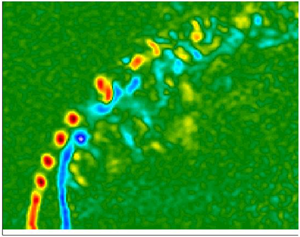
Figure 11 shows instantaneous snapshots of vorticity along the centreplane of the JICF at a momentum flux ratio of $J=5$ for the non-tabbed jet (with the thin round template extension), the tab positioned upstream and the tab downstream. Corresponding mean cross-sectional vorticity images for the same flow and jet geometrical configurations as in figure 11 are shown in figure 12, with images provided at three different downstream locations corresponding to the upstream leading edge of the jet exit ($x/D = -0.5$), the centre of the jet exit ($x/D = 0.0$) and the downstream trailing edge of the jet exit ($x/D = +0.5$). Averaging in these and subsequent mean vorticity images was performed over 500 realizations. For the instantaneous centreplane vorticity without a tab (figure 11a), USL vortex rollup initiated very close to the jet exit, at approximately 0.5 diameters, while the downstream vorticity did not begin to pinch-off until almost 1 diameter after pinch-off in the USL. This vorticity evolution was consistent with that for an AU/GU USL for the nozzle-generated jet in the absence of the thin extension in earlier studies (Gevorkyan et al. Reference Gevorkyan, Shoji, Peng and Karagozian2018), including vorticity magnitude and shear layer instability differences between the windward and leeside of the jet (Davitian et al. Reference Davitian, Getsinger, Hendrickson and Karagozian2010a; Regan & Mahesh Reference Regan and Mahesh2017). The mean cross-sectional vorticity evolution of the jet at three different locations at or near the jet exit in figure 12(a) showed that, in general, the vorticity initiation was relatively symmetric at the upstream edge ($x/D = -0.5$) and at the centre of the jet ($x/D = 0.0$) for the jet without a physical tab. The vorticity at the downstream edge of the jet exit, at $x/D = +0.5$, was slightly asymmetric for the tabless jet, interestingly. This overall behaviour in figure 12(a) was not unexpected given that the USL is naturally AU at $J = 5$ for this jet mixture (Shoji et al. Reference Shoji, Harris, Besnard, Schein and Karagozian2020b), and growth of asymmetries is shown to be suppressed by the larger dominant axisymmetric USL instability mode (Alves et al. Reference Alves, Kelly and Karagozian2007; Regan & Mahesh Reference Regan and Mahesh2017), resulting in symmetric CVP structures at low $J$ values (Getsinger et al. Reference Getsinger, Gevorkyan, Smith and Karagozian2014).

Figure 11.

Centreplane images of the scaled instantaneous vorticity field for the AU jet at $J=5$ and $Re_j=1900$. The colourbars are scaled to the same maximum and minimum vorticity values contained within all images shown. (a) Simple non-tabbed extension. (b) Tab upstream. (c) Tab downstream.

Figure 12.

Mean cross-sectional vorticity images at cross-sectional locations $x/D = -0.5$, $x/D = 0.0$ and $x/D = +0.5$. Images correspond to the (a) non-tabbed jet, (b) tab upstream jet and (c) tab downstream jet, with $J=5$ and $Re_j=1900$. The colourbars are scaled to the maximum and minimum vorticity values contained within each image shown.

When a tab was placed in the upstream edge of the jet at $J=5$, the centreplane instantaneous vorticity image (figure 11b) showed the upstream vorticity initiation to be delayed by 0.50–0.75 diameters, and the overall magnitude of the vorticity in this plane to be significantly weakened as compared with the characteristics shown for the non-tabbed jet (figure 11a). These observations were consistent with the observed delay and significant weakening of USL instabilities for the naturally AU jet at $J=7$ in the high-resolution PLIF results with an upstream tab. Interestingly, in figure 11(b) the upstream tab caused the downstream vorticity dynamics to have approximately the same vortex pinch-off location as for the non-tabbed jet, as well as a slight increase in the maximum downstream vorticity. This may be interpreted by examining the cross-sectional vorticity evolution (figure 12b), where the tab upstream significantly weakened the vorticity generation along the windward side of the jet, shown (as expected) by the vorticity magnitudes at $x/D=-0.5$. But as the jet evolved to the cross-sectional locations $x/D = 0.0$ and $+0.5$, the vorticity actually became slightly stronger than for the non-tabbed jet. The apparent net result of the tab upstream was a dampening of the vorticity generation directly in the upstream region, yet a small but notable increase in vorticity production along the sides and downstream edge of the jet. Though in principle the net vorticity generation from a tab upstream should reorient and act to cancel or at least weaken the CVP, the strengthening of vorticity generation in the downstream region actually created a greater symmetry in the downstream vorticity field and, hence, produced contributions to a symmetric CVP. These observations on the upstream tab were consistent with earlier findings by Zaman (Reference Zaman1998), who found that while the overall circulation from the vorticity isocontours may be lower with the tab upstream, the counter-rotating vortex pair still produces almost identical magnitudes of vorticity at the vortex cores to those for non-tabbed jets. These observations in figure 12(b) were also consistent with and help to explain the high-resolution PLIF-based cross-sectional jet structures for the case in figure 7(b) with an upstream tab at $J = 7$. In this case the CVP becomes only slightly flattened in comparison to the usual symmetric CVP for the non-tabbed transverse jet.

For a transverse jet with a tab placed at the downstream edge of the orifice, both Liscinsky et al. (Reference Liscinsky, True and Holdeman1995) and Zaman & Foss (Reference Zaman and Foss1997) found no difference in the overall vorticity and mixing dynamics compared with the non-tabbed jet, although as noted earlier, their experiments are performed at fairly large momentum flux ratios, exceeding $J = 21$. For a lower momentum flux ratio of $J = 7$ in the high-resolution PLIF experiments, the downstream tab caused the USL to become significantly weaker, as indicated in figure 5(d), transitioning from an absolute instability to a convective instability, although the degree of weakening in the USL was not as significant as that produced by an upstream tab. In the PIV-based vorticity measurements, figure 11(c) indicates that, while the vortex rollup along both the upstream and downstream sides of the jet initiated at nearly the same locations as the non-tabbed jet, the magnitudes of vorticity from both sides of the jet were significantly weakened, consistent with the weakening of the instability characteristics in figure 5(d). The cross-sectional vorticity magnitudes at various downstream locations in figure 12(c) also showed that a downstream tab produced nearly the same overall magnitude of vorticity as that is generated for the non-tabbed jet, and in fact for the most evolved view of the jet at $x/D=+0.5$, the vorticity production was more symmetric than for the non-tabbed jet, though not quite as symmetric as for the upstream tab. Thus, while vorticity directly in the upstream and downstream shear layers was weakened by the downstream tab, the overall vorticity produced in the sides of the jet remained relatively unchanged, leading to the relatively symmetric CVP structure observed far downstream for the case of $J = 7$ in figure 7(c). Hence, there was consistency in the near-field vorticity generation for both centreplane and cross-sectional planes with jet cross-sectional shape in the low $J$ regime.

Figure 13 shows representative instantaneous vorticity fields in the centreplane for larger values of $J$ (8, 20 and 41) for the non-tabbed JICF with a thin extension, as well as for cases with the tab placed upstream and downstream. Figure 14 contains corresponding cross-sectional mean vorticity images at a downstream location $x/D = +0.5$ for these same flow and jet geometrical conditions. This location tended to produce the greatest differences among the different jet configurations. Instantaneous centreplane vorticity images in figure 13 suggested that for each jet configuration, with or without tabs, as the crossflow velocity was reduced (in order to increase $J$), upstream and downstream shear layer rollup was delayed further along the layer, consistent with earlier findings for the round JICF in Getsinger et al. (Reference Getsinger, Gevorkyan, Smith and Karagozian2014) and Gevorkyan et al. (Reference Gevorkyan, Shoji, Peng and Karagozian2018). The upstream tab caused a further delay in the USL vorticity rollup as compared with the non-tabbed case, but for the tab placed downstream at higher $J$ values there was relatively little change, similar to the case for $J = 5$ in figure 11. The magnitudes in figure 13 showed that both upstream and downstream shear layers had a stronger degree of vorticity generation for the non-tabbed case than for either case with tabs.

Figure 13.

Centreplane images of the instantaneous vorticity field for the AU jet near the critical transition at $J=8$ and CU jets at $J=20$ and $J=41$, all with $Re_j=1900$. The colourbars are scaled to the maximum and minimum vorticity values contained within each image shown. (a) Simple extension. (b) Tab upstream. (c) Tab downstream.

Figure 14.

Mean cross-sectional vorticity images at the cross-sectional location $x/D=+0.5$. Images correspond to the (a) non-tabbed jet, (b) tab upstream jet and (c) tab downstream jet, for the AU jet near the critical transition at $J=8$ and CU jets at $J=20$ and $J=41$, all with $Re_j=1900$. The colourbars are scaled to the maximum and minimum vorticity values contained within each image shown.

Cross-sectional mean vorticity fields for the three different configurations, shown for $J = 8$, 20 and 41 in figure 14, indicated that the degree of asymmetry for the non-tabbed jet increased for larger $J$ values, again consistent with prior round JICF observations (Getsinger et al. Reference Getsinger, Gevorkyan, Smith and Karagozian2014). The presence of a tab, either at the upstream or downstream location, tended to make the vorticity field more symmetric, though the results were not exactly the same for these two different tabbed configurations. This near-field cross-sectional symmetry was also seen at lower $J$ values further downstream in high-resolution PLIF results (figure 7b,c). At higher $J$ (figure 8b,c), in contrast, the far-field cross-sections were altered by upstream and downstream tabs, yet were still strongly asymmetric.

Symmetry breaking tab orientations were also explored in simultaneous PLIF/PIV experiments to determine the implications of positioning an asymmetrically oriented tab at the exit plane and thus creating an azimuthal vorticity distribution for the development of the CVP, recalling that Peterson & Plesniak (Reference Peterson and Plesniak2004) suggested such an asymmetric distribution could give rise to asymmetries in the jet further downstream. Recall from figures 7 and 8 that the high-resolution PLIF imaging of a tabbed jet showed that as the tab orientation was azimuthally rotated away from the upstream edge of the jet, the cross-sectional structure showed a bulk deflection of the jet away from the location (right vs left) of the tab, and as the momentum flux ratio increased, the tab was able to produce more pronounced alterations to the naturally asymmetric jet cross-sectional structure. For comparison, figure 15 shows instantaneous centreplane vorticity images and mean cross-sectional vorticity images at $x/D = + 0.5$ for symmetry breaking tab orientations at $J=5$, the flow condition for which tabs had a more dramatic effect on USL instabilities. The centreplane vorticity field showed a rather significant delay in the initiation and strengthening of the USL instabilities and vortex rollup for a tab placed closer to the upstream region (e.g. L15). As the tab was moved azimuthally about the jet periphery, the delay in USL vortex rollup was lessened, to the point where, by position L30 or L45, and definitely by L90 (or R90), there was very little discernible difference with respect to the jet with the non-tabbed simple extension in figure 15. In terms of the mean cross-sectional vorticity in the figure, the azimuthally placed tabs at L15 and L30 tended to introduce asymmetry at the jet exit, generally consistent with asymmetric cross-sectional high-resolution PLIF images of the JICF under similar conditions in figure 7.

Figure 15.

Images of (a) the instantaneous centreplane and (b) mean cross-sectional vorticity fields for $J=5$ and $Re_j=1900$ at $x/D=0.0$. Symmetry breaking tab orientations are shown. The colourbars are scaled to the maximum and minimum vorticity values contained within each image shown.

For the JICF at a higher momentum flux ratio, the naturally asymmetric cross-section was more significantly influenced by specific tab locations. Instantaneous centreplane and mean cross-sectional vorticity fields at $J = 41$ are shown in figure 16. Close inspection indicates that the left and right oriented tabs at the ‘extreme’ conditions L90 and R90 actually produced different delays in the USL vorticity rollup, and the cross-sectional vorticity fields were also different from one another (and were asymmetric with respect to the jet centreplane). These differences were manifested further downstream in high-resolution PLIF experiments in figure 8, with a perceptible deflection of the jet and vorticity field away from the location of the tab. The slight difference in the asymmetric vorticity production between the tab $90^{\circ }$ to the left or right of the upstream may be a result of the inherent asymmetry already present in the transverse jet at $J=41$.

Figure 16.

Images of (a) the instantaneous centreplane and (b) mean cross-sectional vorticity fields for $J=41$ and $Re_j=1900$ at $x/D=0.0$. Selected symmetry breaking tab orientations are shown. The colourbars are scaled to the maximum and minimum vorticity values contained within each image shown.

3.5. POD analysis and counter current shear layer analogy

The tab's influence on other dynamics within the transverse jet flow field may be explored via snapshot POD (Sirovich Reference Sirovich1987) applied to the velocity vector fields from the centreplane stereo-PIV imaging. This approach has been explored in additional studies of the JICF (Meyer, Pedersen & Özcan Reference Meyer, Pedersen and Özcan2007; Schlatter et al. Reference Schlatter, Bagheri and Henningson2011; Gevorkyan et al. Reference Gevorkyan, Shoji, Peng and Karagozian2018) as a means of extracting mode structures from instantaneous snapshots of the flow and identifying dominant instabilities in the flow field. In the present studies, snapshot POD analysis was applied to all 500 instantaneous realizations of the flow field for each test case considered, well above the 300 snapshots required for statistical convergence (Shoji Reference Shoji2017). The resolved mode structures were ordered in terms of their respective magnitudes of total kinetic energy fluctuation, helping to reveal characteristic flow features and dynamics which might otherwise be hidden or masked by the chaotic flow field. Figures 17, 18 and 19 depict the four most energetic mode structures, along with their respective contributions to the total kinetic energy fluctuation, for the transverse jet without a tab, with the tab upstream and with the tab downstream at momentum flux ratios of $J=5$, $J=8$ and $J=41$, respectively. Only $J = 41$ had an USL which was clearly CU in the absence of a tab (Shoji et al. Reference Shoji, Harris, Besnard, Schein and Karagozian2020b). The non-tabbed mode structures over the momentum flux ratio range in question (figures 17a–19a) agreed quite well with the dynamics seen in the snapshot POD for the flush nozzle-injected JICF for the same range by Gevorkyan et al. (Reference Gevorkyan, Shoji, Peng and Karagozian2018), even when the latter did not include a thin circular extension as in the present experiments. In the non-tabbed jet mode plots, for all three $J$ values, the first two most dominant modes displayed isolated structures within the shear layer of the jet, and as the momentum flux ratio decreased, these modes were initiated closer to the jet exit, much like the vortex rollup and shear layer instability characteristics. As noted in Gevorkyan et al. (Reference Gevorkyan, Shoji, Peng and Karagozian2018), such isolation of the mode structures in the shear layer agrees with dynamic mode decomposition analysis of DNS JICF studies by Iyer & Mahesh (Reference Iyer and Mahesh2016). For low momentum flux ratios, especially at $J = 5$ but also at $J = 8$, the structures were contained entirely within the USL of the jet, while at higher momentum flux ratios, as shown by modes one and two at $J=41$ (figure 19a(1)–a(2)), the dominant mode structures spanned the upstream and downstream shear layers, and appeared to be merged. This was analogous to the expansion of the wavemaker region to the downstream shear layer as documented in the DNS by Regan & Mahesh (Reference Regan and Mahesh2019), and the origination of the dominant eignenmode on the downstream side of the jet as shown in Regan & Mahesh (Reference Regan and Mahesh2017), both for a CU jet at $J=16$ and $Re_j=2000$. It is also noted that the wake structures were more pronounced in figures 17(a)–19(a) as the momentum flux ratio was decreased and as the jet became more bent over. The increasing contribution of the wake structures resulted in a decreasing energy content contained within the jet shear layer modes, reducing the energy content within the first mode from $11\,\%$ to $7\,\%$ in changing from $J=41$ to $J=5$. These wake features were most dominant in the non-tabbed jet at $J=5$ (figure 17a(3)–a(4)), where large scale structures denoting in- and out-of-plane velocity form in the jet wake. Gevorkyan et al. (Reference Gevorkyan, Shoji, Peng and Karagozian2018) and Fric & Roshko (Reference Fric and Roshko1994) note such structures are largely associated with the wake vortices which act to entrain crossflow boundary layer fluid up into the jet.

Figure 17.

Particle image velocimetry based POD mode structures extracted from the centreplane velocity field at $J=5$ and $Re_j=1900$, for (a) the non-tabbed jet, (b) the tab upstream and (c) the tab downstream. The respective percentages of total kinetic energy fluctuation content are shown. The colourbar in each image represents the mode scaled by its own norm and the mean jet velocity at the jet exit $U_j$.

Figure 18.

Particle image velocimetry based POD mode structures extracted from the centreplane velocity field at $J=8$ and $Re_j=1900$, for (a) the non-tabbed jet, (b) the tab upstream and (c) the tab downstream. The respective percentages of total kinetic energy fluctuation content are shown. The colourbar in each image represents the mode scaled by its own norm and the mean jet velocity at the jet exit $U_j$.

Figure 19.

Particle image velocimetry based POD mode structures extracted from the centreplane velocity field at $J=41$ and $Re_j=1900$, for (a) the non-tabbed jet, (b) the tab upstream and (c) the tab downstream. The respective percentages of total kinetic energy fluctuation content are shown. The colourbar in each image represents the mode scaled by its own norm and the mean jet velocity at the jet exit $U_j$.

Placement of the tab in the upstream region of the jet exit, as seen in the vorticity field in § 3.4, and in the USL stability (§ 3.1), structure (§ 3.2) and mixing results (§ 2.1) from the high-resolution PLIF experiments, created the most significant alterations to the JICF flow field. The POD modes for each of the corresponding momentum flux ratios ($J = 5$, 8 and 41 in figures 17b, 18b and 19b, respectively) reaffirmed these observations. It was observed that the energy content contained within the first two (nominally shear layer) modes was decreased as compared with the non-tabbed JICF at the same flow conditions, hence, with a weakening of the USL vorticity dynamics. As momentum flux ratio was decreased, the differences in energy content between the non-tabbed and upstream tabbed jets became smaller in magnitude, though the mode structures became much more different from one another, e.g. for the first two modes at $J = 5$ in figure 17. These observations were likely related to the increasing significance of the wake structures as the jet became more bent over, with a transfer of kinetic energy from the USL to the wake structures; this trend was not necessarily associated with the presence of the tab. The overall differences in the most energetic mode shapes for $J = 5$, however, with a broadened region over which oscillations occurred with the upstream tab, were clearly the result of the tab placement. Similar mode shape alterations as well as a transfer of energy from shear layer to wake structures was observed for the upstream tab with $J = 8$ in the figures in 18(b), though to a lesser degree than for $J = 5$. Given that $J=41$ produced a JICF that was largely upright, the presence of wake structures was not detected, and, thus, even in the presence of the tab upstream, did not demonstrate a dramatic decrease in the energy content of the modes. When the tab was placed in the downstream edge of the jet, alterations in the mode structure and energy transfer from the shear layer to the wake were similar to effects observed for the upstream tabs at $J = 8$ and especially at $J = 41$, but there were greater differences between downstream and upstream tab results for $J = 5$. There were clear upstream and downstream mode structures in the first and second POD modes for the downstream tab with $J = 5$ (figure 17c) as compared with the non-tabbed insert in figure 17(a), which only displayed clear USL structures. This observation was consistent with hotwire-based alterations in spectral characteristics of the naturally AU JICF when the tab was placed downstream; the downstream tab as well as the upstream tab weakened the USL's instabilities.

Proper orthogonal decomposition analysis also enables one to analyse the fluctuations in magnitude of the respective mode coefficients across the series of original snapshots, as has been done by Meyer et al. (Reference Meyer, Pedersen and Özcan2007) and Gevorkyan et al. (Reference Gevorkyan, Shoji, Peng and Karagozian2018), and, thus, to study correlations in the evolution of the dynamics in the flow. When treating a specific snapshot image, the magnitude of each respective coefficient represents the contribution of that particular mode in forming a summation from all of the modes to reconstruct the snapshot. If the mode coefficients from select mode pairs are then plotted against one another, it is possible to determine if the respective modes are at all correlated in their evolution over time. Gevorkyan et al. (Reference Gevorkyan, Shoji, Peng and Karagozian2018) demonstrated for the AU jet at $J=5$ that when the first two mode coefficients are plotted against one another for all 500 snapshots, the plot resembles that of a ring, representative of a periodic travelling wave, and that the dominant jet dynamical behaviour may be characterized by linear combinations of the first two modes. For the JICF at larger $J$ values with a CU USL, however, Gevorkyan et al. (Reference Gevorkyan, Shoji, Peng and Karagozian2018) showed that the ring-like plot of the first two mode coefficients deteriorates to a diffuse blob, where no periodic travelling wave behaviour is detectable. Instead the coefficient plots rightly illustrate the broadband frequency content of shear layer instabilities in a CU flow, consistent with corresponding hotwire measurements of the USL. An understanding of the effects of tabs on JICF dynamical characteristics can benefit from this approach as well.

Figure 20 shows plots comparing the coefficients of the first two most energetic proper orthogonal modes for the flow field at $J=5$ for the non-tabbed jet with a simple thin extension, and for tab placements in the upstream, downstream and symmetry breaking tab orientations about the jet exit periphery. Clearly, as was seen by Gevorkyan et al. (Reference Gevorkyan, Shoji, Peng and Karagozian2018) for the flush nozzle-injected jet at $J=5$, the coefficient plot for the non-tabbed jet created a ring, indicative of a travelling wave phenomena associated with the USL structures, as expected for an AU flow. When the tab was then placed in the upstream position, the ring like representation was not recovered, and instead a diffuse blob was formed, typical of a CU flow. This finding was not unexpected in that spectral contour plots from the high-resolution PLIF experiments documented a transition in the USL instabilities from absolute to convective instability with the tab upstream for $J=7$ and $Re_j=2300$. There was also a slight transition in the shear layer instabilities when the tab was positioned downstream, although the coefficient plots retained the ring shape overall, suggesting here that the flow remained AU at $J = 5$ for such a tab placement. The high-resolution PLIF instability characteristics in figure 5(d) were actually for a momentum flux ratio closer to the critical transition between absolute and convective instability ($J = 7$), and, hence, was more likely to be affected by small alterations in the flow such as a downstream tab. In contrast, the momentum flux ratio of $J=5$ in the simultaneous imaging experiments was more strongly AU and, thus, further from the critical transition for these flow conditions. Hence, for the strong AU flow at $J = 5$, the weaker influence of the tab downstream resulted in the flow's remaining AU in POD mode coefficient plots. This observation was also seen in the USL vorticity generation for the downstream tab at $J = 5$ in figure 11; its instantaneous structure was remarkably similar to that of the non-tabbed jet, but was quite different from that of the tab positioned at the upstream. The coefficient plots in figure 21 for $J = 8$ reinforced this idea of the impact of the tab being dependent on the closeness of the USL instability state to absolute instability conditions. The non-tabbed jet here was still AU, though more weakly so as it was closer to the critical transition around $J\approx 9\text {--}10$, and when the tab was placed in either the upstream or downstream, the resulting coefficient plot showed more diffuse blobs rather than a circle, as would be expected for a flow field that was CU. Further extension of this evaluation to tab configurations at $J=41$ in figure 22 showed the expected diffuse blobs in the coefficient plots for all tab orientations, as the flow is known to be naturally CU, and the tab acted to further weaken the flow field instabilities.

Figure 20.

Particle image velocimetry based POD coefficients of the first two modes plotted against each other. Data are extracted from the centreplane velocity field at $J=5$ and $Re_j=1900$, for a variety of tab configurations. (a) Simple extension. (b) Tab upstream. (c) Tab downstream. Other tab locations are as labelled.

Figure 21.

Particle image velocimetry based POD coefficients of the first two modes plotted against each other. Data are extracted from the centreplane velocity field at $J=8$ and $Re_j=1900$, for a variety of tab configurations. (a) Simple extension. (b) Tab upstream. (c) Tab downstream. Other tab locations are as labelled.

Figure 22.

Particle image velocimetry based POD coefficients of the first two modes plotted against each other. Data are extracted from the centreplane velocity field at $J=41$ and $Re_j=1900$, for a variety of tab configurations. (a) Simple extension. (b) Tab upstream. (c) Tab downstream. Other tab locations are as labelled.

Interestingly, the resulting coefficient plots for symmetry breaking tab orientations for all three momentum flux ratios were generally consistent with the trends in USL spectra from the high-resolution PLIF experiments in § 3.1, as well as the vorticity analysis in § 3.4, demonstrating that the influence of the tab was most significant when the USL was naturally strongly AU. For the flow at $J=5$, in figure 20, besides the upstream tab, there were additional alterations in the coefficient plots, though not as severe, when the tab was situated at L15 and L45 positions. Separate studies (Harris Reference Harris2020) show downstream cross-sectional asymmetries for such cases, with a more significant bulk deflection of the CVP. The altered (non-blob-like) structures for these two cases in figure 20 suggested additional complexity in the dynamics that could warrant further exploration. As for the other cases, for $J = 8$ in figure 21, only the downstream, L30, and possibly L60 tab configurations showed some evidence of periodicity in the flow, while other cases indicated weakening of the disturbances to become like a CU flow field. For $J = 41$ in figure 22, the coefficient plots showed no significant alterations with the presence of tabs at any position, generally consistent with spectral characteristics and centreplane imaging for the CU JICF from the high-resolution PLIF experiments.

In addition to the vorticity field and POD analysis of the velocity field extracted from the present experiments, the local velocity field in the vicinity of the upstream region of the jet exit for different tab (and tabless) configurations was also examined. The origins of the transition in the transverse jet's USL instabilities can be understood in the context of viewing the USL near the flush jet exit as a counter-current shear layer (CCSL) where the effect of blockage of the crossflow by the jet column creates a local negative velocity upstream of the USL adjacent to a local positive vertical velocity within the jet, per the ideas of Iyer & Mahesh (Reference Iyer and Mahesh2016). When the CCSL velocity ratio is large enough, the counterflow between the streams can create transition from convective to absolute instability in the shear layer, as one would observe for the planar CCSL (Huerre & Monkewitz Reference Huerre and Monkewitz1985; Strykowski & Niccum Reference Strykowski and Niccum1991). Extensive experimental studies of this near-field region of the JICF for a range of $J$ values in Shoji et al. (Reference Shoji, Harris, Besnard, Schein and Karagozian2020b) demonstrated a general consistency in the CCSL model in understanding transverse jet USL transition to absolute instability. Shoji et al. (Reference Shoji, Harris, Besnard, Schein and Karagozian2020b) also demonstrated that as the upstream momentum thickness of the exiting jet becomes larger, the degree or strength of counter-current flow required to cause transition from CU to AU increases. Hence, for the same crossflow and jet bulk velocity conditions, a thicker upstream momentum thickness $\theta$ could create a weaker instability in the USL; this is also consistent with a diminished growth rate of the axisymmetric instability mode for the high momentum flux ratio JICF (Alves et al. Reference Alves, Kelly and Karagozian2008). Such measurements of the velocity in these experiments enabled exploration of the influence of the tabs on the local USL flow field in the context changes in the jet's upstream momentum thickness.

To explore the effect of a tab placed at various locations on the upstream jet momentum thickness $\theta$, the velocity field in the $x\text {--}z$ plane at the upstream region of the jet near the jet exit, extracted from PIV measurements, was used, with details on the method of extraction described in Shoji et al. (Reference Shoji, Harris, Besnard, Schein and Karagozian2020b). This method was applied to all jet configurations here, including a range of tab positions. The results for $J = 5$ for various tab orientations are given in table 1, where the scaled upstream momentum thickness $\theta / D$, and state of the USL as determined via hotwire anemometry (AU or CU) are given. The data in table 1, and the corresponding data for $J = 8$ in table 2, showed a correspondence between the larger values of $\theta$ and the observed state of the USL per hotwire measurements, which, interestingly, were also consistent with the POD coefficient plots. Even when the tab was placed azimuthally at a position well away from the jet's USL, the small and moderate increases in upstream momentum thickness $\theta$ were consistent with the altered state of the jet's dynamics as observed in the hotwire measurements and in POD coefficient plots. We also note that the momentum thickness of the jet was significantly increased over the non-tabbed jet when the tab was upstream, and moderately so when the tab was downstream. Thickening of the momentum thickness was typically reduced as the tab orientation was rotated away from the upstream, having the least impact when placed directly in the sides of the jet. As stated for the POD coefficient plots, some unusual behaviour in the shear layer dynamics may be due to the large asymmetric deflection of the jet structure, whereby the shear layer dynamics were not entirely captured in the centreplane view of the evolving jet. Also possible is that asymmetric instabilities may be initiated and growing to compete with the axisymmetric mode, such that analysis of the periodicity of the USL from the coefficient plots may not be accurately recovered due to coupling of the instability modes, which would contaminate the simple periodic behaviour.

Table 1.

For $J = 5$ and $Re_j = 1900$, the upstream jet momentum thickness at the jet exit (scaled by $D$) and the hotwire-based state of the USL.

Table 2.

For $J = 8$ and $Re_j = 1900$, the upstream jet momentum thickness at the jet exit (scaled by $D$) and the hotwire-based state of the USL.