2.1 Problem definition

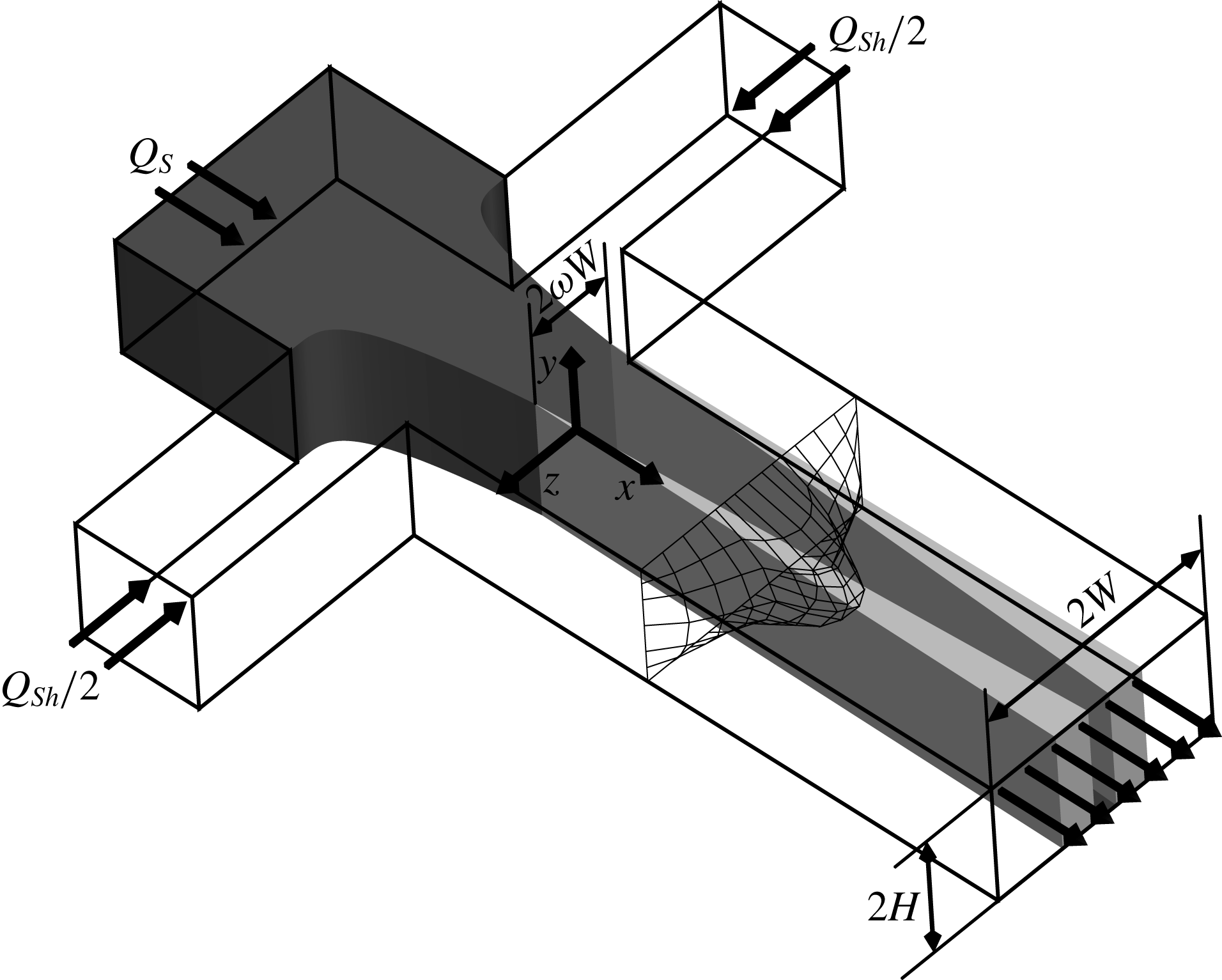
The steady-state solute concentration in two-dimensional hydrodynamic focusing is theoretically investigated. The schematic of the problem, including the dimensions and the coordinate system, is illustrated in figure 1. As shown, the main channel is rectangular with a width of $2W$ and a height of $2H$ . The sample flow, including a species of concentration $c_{0}$ , enters the junction from the central channel and is sandwiched between two sheath flows issued from the side inlets. The sample flow is considered to have a dynamic viscosity of $\unicode[STIX]{x1D707}_{S}$ and a volumetric flow rate of $Q_{S}$ . Each sheath stream, with dynamic viscosity $\unicode[STIX]{x1D707}_{Sh}$ , has a flow rate of $Q_{Sh}/2$ . The origin of the coordinate system is located at the centre of the channel cross-sectional area at the end of the focusing region where the flow no longer changes with $x$ . The portion of the channel width occupied by the sample flow at the end of the focusing region is $\unicode[STIX]{x1D714}$ , so that the width of the sample stream is $2\unicode[STIX]{x1D714}W$ . Note that the stratified flow in straight microchannels has been found to be stable via extensive experiments (Cubaud & Mason Reference Cubaud and Mason2012); so assuming a constant $\unicode[STIX]{x1D714}$ for $0\leqslant x$ seems reasonable.

Figure 1.

Schematic of the hydrodynamic focusing device considered including the dimensions, the coordinate system, and a typical velocity profile. The fluid containing solutes, referred to as sample fluid, enters the main channel from the middle inlet with volumetric flow rate $Q_{S}$ . The sheath streams enter the device from the side inlets with a flow rate of $Q_{Sh}/2$ each. The darkness of the shading denotes solute abundance, which is lower in two diffusion zones created at the sample–sheath interfaces.

Table 1.

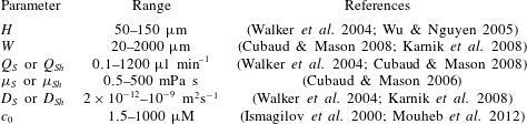
Typical ranges of the main governing parameters.

The typical parameter values are given in table 1. Based on the dimensions provided, the size-less particle assumption holds since the molecular size of the solutes, typically within nanometres (Kamholz et al. Reference Kamholz, Weigl, Finlayson and Yager1999), is considerably smaller than the minimum channel dimension encountered in real applications. We assume that the sample and sheath fluids are immiscible and the resulting flows are laminar and incompressible. Furthermore, the influence of interfacial tension may be regarded as negligible since the curvature of the interface in stratified flows is very small (Datta, Gada & Sharma Reference Datta, Gada and Sharma2011). The partitioning effect is also neglected so that the solute concentration may be assumed continuous at the liquid–liquid interfaces (Wu & Nguyen Reference Wu and Nguyen2005). Additionally, although the existence of the species in the flow introduces some nonlinear rheological effects, the fluids may still be considered as Newtonian, as the solute concentration is low in the practical applications. Low solute concentrations also enable us to assume the effect of the solute concentration on the fluid viscosity is negligible, and to consider the fluids to have constant dynamic viscosities. This may be illustrated as follows. Assuming that the solute concentration is low, the solution viscosity becomes $\unicode[STIX]{x1D707}=\unicode[STIX]{x1D707}_{0}(1+[\unicode[STIX]{x1D707}]c^{\ast \ast })$ wherein $c^{\ast \ast }$ is the solute concentration in $\text{g}~\text{dl}^{-1}$ , $\unicode[STIX]{x1D707}_{0}$ is the solvent viscosity, and $[\unicode[STIX]{x1D707}]$ is the intrinsic viscosity, which equals $2.5~\text{dl}~\text{g}^{-1}$ for a solution of rigid spherical particles (Jeffery Reference Jeffery1922; Riseman & Ullman Reference Riseman and Ullman1951). Converting the maximum practical value of $c_{0}$ in table 1 to a mass concentration utilizing a molar mass of $100~\text{g}~\text{mol}^{-1}$ , $c^{\ast \ast }$ becomes $0.01~\text{g}~\text{dl}^{-1}$ , resulting in 2.5 % increase of the dynamic viscosity which is quite small. Finally, following Wu & Nguyen (Reference Wu and Nguyen2005), it is assumed that the focusing length is small compared to the channel length so that the cross-stream diffusion is negligible for $x\leqslant 0$ .

2.2 Velocity distribution

2.2.1 General solution

Solving the momentum equation for the sample and sheath flows separately subject to appropriate boundary and interfacial conditions is a common method of obtaining the velocity distribution in two-phase hydrodynamic focusing. This method, however, leads to expressions that go to infinity for limiting values of the governing parameters and, hence, are very difficult to be calculated (Tripathi et al. Reference Tripathi, Chakravarty and Agrawal2014). Moreover, since a single-domain formulation is implemented for the mass transport analysis, it is more convenient to use the same approach for the hydrodynamic features. In the single-domain formulation, in which the fluid area is considered as a single medium with variable physical properties, the axial momentum equation corresponding to fully developed flow is

(2.1) $$\begin{eqnarray}{\displaystyle \frac{\unicode[STIX]{x2202}}{\unicode[STIX]{x2202}y}}\left(\unicode[STIX]{x1D707}{\displaystyle \frac{\unicode[STIX]{x2202}u}{\unicode[STIX]{x2202}y}}\right)+{\displaystyle \frac{\unicode[STIX]{x2202}}{\unicode[STIX]{x2202}z}}\left(\unicode[STIX]{x1D707}{\displaystyle \frac{\unicode[STIX]{x2202}u}{\unicode[STIX]{x2202}z}}\right)-{\displaystyle \frac{\unicode[STIX]{x2202}p}{\unicode[STIX]{x2202}x}}=0.\end{eqnarray}$$

Here, $u$ is the axial velocity, $p$ stands for the pressure, and $\unicode[STIX]{x1D707}(y,z)$ is the dynamic viscosity that may be dependent upon both lateral coordinates. Considering dimensionless factors $y^{\ast }=y/W$ , $z^{\ast }=z/W$ , $u^{\ast }=-u\unicode[STIX]{x1D707}_{S}/(\unicode[STIX]{x2202}p/\unicode[STIX]{x2202}x)W^{2}$ and $\unicode[STIX]{x1D707}^{\ast }=\unicode[STIX]{x1D707}/\unicode[STIX]{x1D707}_{S}$ , the momentum conservation equation is scaled as

(2.2) $$\begin{eqnarray}{\displaystyle \frac{\unicode[STIX]{x2202}}{\unicode[STIX]{x2202}y^{\ast }}}\left(\unicode[STIX]{x1D707}^{\ast }{\displaystyle \frac{\unicode[STIX]{x2202}u^{\ast }}{\unicode[STIX]{x2202}y^{\ast }}}\right)+{\displaystyle \frac{\unicode[STIX]{x2202}}{\unicode[STIX]{x2202}z^{\ast }}}\left(\unicode[STIX]{x1D707}^{\ast }{\displaystyle \frac{\unicode[STIX]{x2202}u^{\ast }}{\unicode[STIX]{x2202}z^{\ast }}}\right)+1=0.\end{eqnarray}$$

Equation (2.2) must be solved subject to the following boundary and symmetry conditions

(2.3) $$\begin{eqnarray}\left.{\displaystyle \frac{\unicode[STIX]{x2202}u^{\ast }}{\unicode[STIX]{x2202}y^{\ast }}}\right|_{y^{\ast }=0}=\left.{\displaystyle \frac{\unicode[STIX]{x2202}u^{\ast }}{\unicode[STIX]{x2202}z^{\ast }}}\right|_{z^{\ast }=0}=u^{\ast }|_{y^{\ast }=\unicode[STIX]{x1D6FC}}=u^{\ast }|_{z^{\ast }=1}=0,\end{eqnarray}$$

where $\unicode[STIX]{x1D6FC}=H/W$ is the aspect ratio of the main channel. The first two boundary conditions in (2.3) arise from the symmetry at the midplanes and the remaining conditions represent the no-slip conditions at the channel walls. Note that the sample–sheath interfaces are now internal regions and interfacial conditions do not need to be specified. We make use of variational calculus for solving (2.2) subject to the boundary conditions (2.3). The solution is sought from the minimization of the following functional (Haji-Sheikh, Sparrow & Minkowycz Reference Haji-Sheikh, Sparrow and Minkowycz2005; Haji-Sheikh Reference Haji-Sheikh2009)

(2.4) $$\begin{eqnarray}\displaystyle I_{u} & = & \displaystyle \displaystyle \int _{\mathbb{A}^{\ast }}\left\{\unicode[STIX]{x1D707}^{\ast }\left({\displaystyle \frac{\unicode[STIX]{x2202}u^{\ast }}{\unicode[STIX]{x2202}y^{\ast }}}\right)^{2}+\unicode[STIX]{x1D707}^{\ast }\left({\displaystyle \frac{\unicode[STIX]{x2202}u^{\ast }}{\unicode[STIX]{x2202}z^{\ast }}}\right)^{2}-2u^{\ast }\right.\nonumber\\ \displaystyle & & \displaystyle -\,\left.{\displaystyle \frac{1}{2}}\left[{\displaystyle \frac{\unicode[STIX]{x2202}}{\unicode[STIX]{x2202}y^{\ast }}}\left(\unicode[STIX]{x1D707}^{\ast }{\displaystyle \frac{\unicode[STIX]{x2202}u^{\ast 2}}{\unicode[STIX]{x2202}y^{\ast }}}\right)+{\displaystyle \frac{\unicode[STIX]{x2202}}{\unicode[STIX]{x2202}z^{\ast }}}\left(\unicode[STIX]{x1D707}^{\ast }{\displaystyle \frac{\unicode[STIX]{x2202}u^{\ast 2}}{\unicode[STIX]{x2202}z^{\ast }}}\right)\right]\!\right\}\,\text{d}\mathbb{A}^{\ast }.\end{eqnarray}$$

Note that $I_{u}=\int _{\mathbb{A}^{\ast }}F\,\text{d}\mathbb{A}^{\ast }$ is constructed so that

(2.5) $$\begin{eqnarray}\displaystyle & & \displaystyle \unicode[STIX]{x2202}\mathbb{F}/\unicode[STIX]{x2202}u^{\ast }-\unicode[STIX]{x2202}(\unicode[STIX]{x2202}\mathbb{F}/\unicode[STIX]{x2202}u_{y^{\ast }}^{\ast })/\unicode[STIX]{x2202}y^{\ast }-\unicode[STIX]{x2202}(\unicode[STIX]{x2202}\mathbb{F}/\unicode[STIX]{x2202}u_{z^{\ast }}^{\ast })/\unicode[STIX]{x2202}z^{\ast }\nonumber\\ \displaystyle & & \displaystyle \quad +\,\unicode[STIX]{x2202}^{2}(\unicode[STIX]{x2202}\mathbb{F}/\unicode[STIX]{x2202}u_{y^{\ast }y^{\ast }}^{\ast })/\unicode[STIX]{x2202}y^{\ast 2}+\unicode[STIX]{x2202}^{2}(\unicode[STIX]{x2202}\mathbb{F}/\unicode[STIX]{x2202}u_{z^{\ast }z^{\ast }}^{\ast })/\unicode[STIX]{x2202}z^{\ast 2}=0\end{eqnarray}$$

reduces to (2.2) (Weber & Arfken Reference Weber and Arfken2003). In (2.5), the subscripts $y^{\ast }$ and $z^{\ast }$ denote partial differentiation with respect to these variables. The conversion of the differential equation into an integral over the dimensionless form of the cross-sectional area $\mathbb{A}$ , given as $\mathbb{A}^{\ast }=\mathbb{A}/W^{2}$ , is the key factor in bypassing the difficulties associated with matching different solutions of a multidomain region. We consider $u^{\ast }$ as a composition of a complete and linearly independent set of basis functions $\unicode[STIX]{x1D557}_{lm}(y^{\ast },z^{\ast })$ as

(2.6) $$\begin{eqnarray}u^{\ast }=\mathop{\sum }_{l=0}^{l_{max}}\mathop{\sum }_{m=0}^{m_{max}}\unicode[STIX]{x1D555}_{lm}\unicode[STIX]{x1D557}_{lm}.\end{eqnarray}$$

One may select any form for the basis functions provided the boundary conditions (2.3) are satisfied without imposing unphysical constraints on the solution. Due to the ease of using the trigonometric functions, $\unicode[STIX]{x1D557}_{lm}$ is considered to be

(2.7) $$\begin{eqnarray}\unicode[STIX]{x1D557}_{lm}(y^{\ast },z^{\ast })=\cos (\unicode[STIX]{x1D709}_{l}y^{\ast }/\unicode[STIX]{x1D6FC})\cos (\unicode[STIX]{x1D709}_{m}z^{\ast }),\end{eqnarray}$$

where $\unicode[STIX]{x1D709}_{l}=(2l+1)\unicode[STIX]{x03C0}/2$ and $\unicode[STIX]{x1D709}_{m}=(2m+1)\unicode[STIX]{x03C0}/2$ . Since the variational approaches require a single series set of the basis functions, we rewrite (2.6) as

(2.8) $$\begin{eqnarray}u^{\ast }=\mathop{\sum }_{j=1}^{N}d_{j}\,f_{j},\end{eqnarray}$$

where $d_{j}=\unicode[STIX]{x1D555}_{lm}$ and $f_{j}=\unicode[STIX]{x1D557}_{lm}$ . The index $j$ in (2.8) is considered as $j=1+m+l(m_{max}+1)$ so that by varying $m$ between 0 and $m_{max}$ and $l$ between 0 and $l_{max}$ the variable $j$ ranges from 1 to $N=(l_{max}+1)(m_{max}+1)$ , implying that all the terms of the double series form (2.6) are covered by (2.8).

In the subsequent formulation, it frequently occurs that two basis functions or their derivatives are multiplied together. Hence, besides $j$ , it is required to introduce another index for $f$ , say $i$ , to distinguish between different basis functions. Since it is also required to distinguish the parameters $l$ and $m$ and, consequently, $\unicode[STIX]{x1D709}_{l}$ and $\unicode[STIX]{x1D709}_{m}$ pertinent to these indices, each index is shown as a subscript of the associated parameters. In other words, the parameters $l$ and $m$ pertinent to index $i$ are shown as $l_{i}$ and $m_{i}$ , while those of $f_{j}$ are denoted as $l_{j}$ and $m_{j}$ .

Since $I_{u}$ is a function of $d_{1},d_{2},\ldots ,d_{N}$ , its minimization requires

(2.9) $$\begin{eqnarray}{\displaystyle \frac{\unicode[STIX]{x2202}I_{u}}{\unicode[STIX]{x2202}d_{i}}}=0\quad \text{for }i=1,2,\ldots ,N,\end{eqnarray}$$

which leads to

(2.10) $$\begin{eqnarray}\displaystyle & & \displaystyle 2\displaystyle \int _{\mathbb{A}^{\ast }}\left(\unicode[STIX]{x1D707}^{\ast }{\displaystyle \frac{\unicode[STIX]{x2202}u^{\ast }}{\unicode[STIX]{x2202}y^{\ast }}}{\displaystyle \frac{\unicode[STIX]{x2202}f_{i}}{\unicode[STIX]{x2202}y^{\ast }}}+\unicode[STIX]{x1D707}^{\ast }{\displaystyle \frac{\unicode[STIX]{x2202}u^{\ast }}{\unicode[STIX]{x2202}z^{\ast }}}{\displaystyle \frac{\unicode[STIX]{x2202}f_{i}}{\unicode[STIX]{x2202}z^{\ast }}}-f_{i}\right)\text{d}\mathbb{A}^{\ast }\nonumber\\ \displaystyle & & \displaystyle \quad -\,\displaystyle \int _{\mathbb{A}^{\ast }}\left\{{\displaystyle \frac{\unicode[STIX]{x2202}}{\unicode[STIX]{x2202}y^{\ast }}}\left[\unicode[STIX]{x1D707}^{\ast }{\displaystyle \frac{\unicode[STIX]{x2202}(u^{\ast }f_{i})}{\unicode[STIX]{x2202}y^{\ast }}}\right]+{\displaystyle \frac{\unicode[STIX]{x2202}}{\unicode[STIX]{x2202}z^{\ast }}}\left[\unicode[STIX]{x1D707}^{\ast }{\displaystyle \frac{\unicode[STIX]{x2202}(u^{\ast }f_{i})}{\unicode[STIX]{x2202}z^{\ast }}}\right]\!\right\}\text{d}\mathbb{A}^{\ast }=0\nonumber\\ \displaystyle & & \displaystyle \qquad \text{for }i=1,2,\ldots ,N.\end{eqnarray}$$

The second integral in (2.10) may be rewritten as

(2.11) $$\begin{eqnarray}\displaystyle & & \displaystyle \displaystyle \int _{\mathbb{A}^{\ast }}\left\{{\displaystyle \frac{\unicode[STIX]{x2202}}{\unicode[STIX]{x2202}y^{\ast }}}\left[\unicode[STIX]{x1D707}^{\ast }{\displaystyle \frac{\unicode[STIX]{x2202}(u^{\ast }f_{i})}{\unicode[STIX]{x2202}y^{\ast }}}\right]+{\displaystyle \frac{\unicode[STIX]{x2202}}{\unicode[STIX]{x2202}z^{\ast }}}\left[\unicode[STIX]{x1D707}^{\ast }{\displaystyle \frac{\unicode[STIX]{x2202}(u^{\ast }f_{i})}{\unicode[STIX]{x2202}z^{\ast }}}\right]\!\right\}\text{d}\mathbb{A}^{\ast }\nonumber\\ \displaystyle & & \displaystyle \qquad =\displaystyle \int _{\mathbb{A}^{\ast }}\unicode[STIX]{x1D735}^{\ast }\boldsymbol{\cdot }\left[\unicode[STIX]{x1D707}^{\ast }\unicode[STIX]{x1D735}^{\ast }(u^{\ast }f_{i})\right]\text{d}\mathbb{A}^{\ast }=\displaystyle \int _{\mathbb{P}^{\ast }}\unicode[STIX]{x1D707}^{\ast }\left(f_{i}{\displaystyle \frac{\unicode[STIX]{x2202}u^{\ast }}{\unicode[STIX]{x2202}\unicode[STIX]{x1D55F}^{\ast }}}+u^{\ast }{\displaystyle \frac{\unicode[STIX]{x2202}f_{i}}{\unicode[STIX]{x2202}\unicode[STIX]{x1D55F}^{\ast }}}\right)\text{d}\mathbb{P}^{\ast },\end{eqnarray}$$

where $\mathbb{P}^{\ast }=\mathbb{P}/W$ stands for the dimensionless form of the perimeter $\mathbb{P}$ and $\unicode[STIX]{x1D55F}^{\ast }=\unicode[STIX]{x1D55F}/W$ denotes the dimensionless form of $\unicode[STIX]{x1D55F}$ which measures the outward distance in the direction normal to the perimeter. The basis functions satisfy the symmetry and no-slip boundary conditions, so that the line integral in (2.11) is zero. Substituting for $u^{\ast }$ in (2.10) from (2.8) then gives

(2.12) $$\begin{eqnarray}\mathop{\sum }_{j=1}^{N}d_{j}\displaystyle \int _{\mathbb{A}^{\ast }}\left(\unicode[STIX]{x1D707}^{\ast }{\displaystyle \frac{\unicode[STIX]{x2202}f_{i}}{\unicode[STIX]{x2202}y^{\ast }}}{\displaystyle \frac{\unicode[STIX]{x2202}f_{j}}{\unicode[STIX]{x2202}y^{\ast }}}+\unicode[STIX]{x1D707}^{\ast }{\displaystyle \frac{\unicode[STIX]{x2202}f_{i}}{\unicode[STIX]{x2202}z^{\ast }}}{\displaystyle \frac{\unicode[STIX]{x2202}f_{j}}{\unicode[STIX]{x2202}z^{\ast }}}\right)\text{d}\mathbb{A}^{\ast }=\displaystyle \int _{\mathbb{ A}^{\ast }}f_{i}\,\text{d}\mathbb{A}^{\ast }\quad \text{for }i=1,2,\ldots ,N.\end{eqnarray}$$

This equation represents a system of $N$ equations for the $N$ unknowns $d_{1}$ to $d_{N}$ . This system may be written in matrix form as

(2.13) $$\begin{eqnarray}\unicode[STIX]{x1D63D}\boldsymbol{d}=\boldsymbol{E},\end{eqnarray}$$

where $\boldsymbol{d}$ is the vector of coefficients $d_{1},d_{2},\ldots ,d_{N}$ and the elements of the matrix $\unicode[STIX]{x1D63D}$ and vector $\boldsymbol{E}$ are determined by

(2.14) $$\begin{eqnarray}\displaystyle & \displaystyle b_{ij}=\displaystyle \int _{\mathbb{A}^{\ast }}\left(\unicode[STIX]{x1D707}^{\ast }{\displaystyle \frac{\unicode[STIX]{x2202}f_{i}}{\unicode[STIX]{x2202}y^{\ast }}}{\displaystyle \frac{\unicode[STIX]{x2202}f_{j}}{\unicode[STIX]{x2202}y^{\ast }}}+\unicode[STIX]{x1D707}^{\ast }{\displaystyle \frac{\unicode[STIX]{x2202}f_{i}}{\unicode[STIX]{x2202}z^{\ast }}}{\displaystyle \frac{\unicode[STIX]{x2202}f_{j}}{\unicode[STIX]{x2202}z^{\ast }}}\right)\text{d}\mathbb{A}^{\ast }, & \displaystyle\end{eqnarray}$$

(2.15) $$\begin{eqnarray}\displaystyle & \displaystyle e_{i}=\displaystyle \int _{\mathbb{A}^{\ast }}f_{i}\,\text{d}\mathbb{A}^{\ast }. & \displaystyle\end{eqnarray}$$

It is easy to verify that $e_{i}$ is of the following form

(2.16) $$\begin{eqnarray}e_{i}={\displaystyle \frac{\unicode[STIX]{x1D6FC}(-1)^{l_{i}+m_{i}}}{\unicode[STIX]{x1D709}_{l_{i}}\unicode[STIX]{x1D709}_{m_{i}}}}.\end{eqnarray}$$

To evaluate $b_{ij}$ , the integral is separated into two parts, one over the dimensionless sample stream area $\mathbb{A}_{S}^{\ast }$ within which $\unicode[STIX]{x1D707}^{\ast }=\unicode[STIX]{x1D707}_{S}/\unicode[STIX]{x1D707}_{S}=1$ and the other over the dimensionless sheath flow area $\mathbb{A}_{Sh}^{\ast }$ with $\unicode[STIX]{x1D707}^{\ast }=\unicode[STIX]{x1D707}_{Sh}/\unicode[STIX]{x1D707}_{S}=\unicode[STIX]{x1D702}_{\unicode[STIX]{x1D707}}$ , so that

(2.17) $$\begin{eqnarray}b_{ij}=\displaystyle \int _{\mathbb{A}_{S}^{\ast }}\left({\displaystyle \frac{\unicode[STIX]{x2202}f_{i}}{\unicode[STIX]{x2202}y^{\ast }}}{\displaystyle \frac{\unicode[STIX]{x2202}f_{j}}{\unicode[STIX]{x2202}y^{\ast }}}+{\displaystyle \frac{\unicode[STIX]{x2202}f_{i}}{\unicode[STIX]{x2202}z^{\ast }}}{\displaystyle \frac{\unicode[STIX]{x2202}f_{j}}{\unicode[STIX]{x2202}z^{\ast }}}\right)\text{d}\mathbb{A}^{\ast }+\unicode[STIX]{x1D702}_{\unicode[STIX]{x1D707}}\displaystyle \int _{\mathbb{ A}_{Sh}^{\ast }}\left({\displaystyle \frac{\unicode[STIX]{x2202}f_{i}}{\unicode[STIX]{x2202}y^{\ast }}}{\displaystyle \frac{\unicode[STIX]{x2202}f_{j}}{\unicode[STIX]{x2202}y^{\ast }}}+{\displaystyle \frac{\unicode[STIX]{x2202}f_{i}}{\unicode[STIX]{x2202}z^{\ast }}}{\displaystyle \frac{\unicode[STIX]{x2202}f_{j}}{\unicode[STIX]{x2202}z^{\ast }}}\right)\text{d}\mathbb{A}^{\ast }.\end{eqnarray}$$

We then find that

(2.18) $$\begin{eqnarray}\displaystyle b_{ij} & = & \displaystyle \unicode[STIX]{x1D6FF}_{l_{i},l_{j}}(1-\unicode[STIX]{x1D6FF}_{m_{i},m_{j}})\left\{{\displaystyle \frac{\unicode[STIX]{x1D709}_{l_{i}}^{2}(1-\unicode[STIX]{x1D702}_{\unicode[STIX]{x1D707}})}{4\unicode[STIX]{x1D6FC}}}\left\{{\displaystyle \frac{\sin [(\unicode[STIX]{x1D709}_{m_{i}}-\unicode[STIX]{x1D709}_{m_{j}})\unicode[STIX]{x1D714}]}{\unicode[STIX]{x1D709}_{m_{i}}-\unicode[STIX]{x1D709}_{m_{j}}+\unicode[STIX]{x1D6FF}_{m_{i},m_{j}}}}+{\displaystyle \frac{\sin [(\unicode[STIX]{x1D709}_{m_{i}}+\unicode[STIX]{x1D709}_{m_{j}})\unicode[STIX]{x1D714}]}{\unicode[STIX]{x1D709}_{m_{i}}+\unicode[STIX]{x1D709}_{m_{j}}}}\right\}\right.\nonumber\\ \displaystyle & & \displaystyle \left.+\,{\displaystyle \frac{\unicode[STIX]{x1D6FC}\unicode[STIX]{x1D709}_{m_{i}}\unicode[STIX]{x1D709}_{m_{j}}(1-\unicode[STIX]{x1D702}_{\unicode[STIX]{x1D707}})}{4}}\left\{{\displaystyle \frac{\sin [(\unicode[STIX]{x1D709}_{m_{i}}-\unicode[STIX]{x1D709}_{m_{j}})\unicode[STIX]{x1D714}]}{\unicode[STIX]{x1D709}_{m_{i}}-\unicode[STIX]{x1D709}_{m_{j}}+\unicode[STIX]{x1D6FF}_{m_{i},m_{j}}}}-{\displaystyle \frac{\sin \left[(\unicode[STIX]{x1D709}_{m_{i}}+\unicode[STIX]{x1D709}_{m_{j}})\unicode[STIX]{x1D714}\right]}{\unicode[STIX]{x1D709}_{m_{i}}+\unicode[STIX]{x1D709}_{m_{j}}}}\right\}\!\right\}\nonumber\\ \displaystyle & & \displaystyle +\,\unicode[STIX]{x1D6FF}_{l_{i},l_{j}}\unicode[STIX]{x1D6FF}_{m_{i},m_{j}}\left\{{\displaystyle \frac{\unicode[STIX]{x1D6FC}\unicode[STIX]{x1D702}_{\unicode[STIX]{x1D707}}\unicode[STIX]{x1D709}_{m_{i}}^{2}}{4}}+{\displaystyle \frac{\unicode[STIX]{x1D702}_{\unicode[STIX]{x1D707}}\unicode[STIX]{x1D709}_{l_{i}}^{2}}{4\unicode[STIX]{x1D6FC}}}+{\displaystyle \frac{\unicode[STIX]{x1D709}_{l_{i}}^{2}(1-\unicode[STIX]{x1D702}_{\unicode[STIX]{x1D707}})}{4\unicode[STIX]{x1D6FC}}}\left[\unicode[STIX]{x1D714}+{\displaystyle \frac{\sin (2\unicode[STIX]{x1D709}_{m_{i}}\unicode[STIX]{x1D714})}{2\unicode[STIX]{x1D709}_{m_{i}}}}\right]\right.\nonumber\\ \displaystyle & & \displaystyle \left.+\,{\displaystyle \frac{\unicode[STIX]{x1D6FC}\unicode[STIX]{x1D709}_{m_{i}}^{2}(1-\unicode[STIX]{x1D702}_{\unicode[STIX]{x1D707}})}{4}}\left[\unicode[STIX]{x1D714}-{\displaystyle \frac{\sin (2\unicode[STIX]{x1D709}_{m_{i}}\unicode[STIX]{x1D714})}{2\unicode[STIX]{x1D709}_{m_{i}}}}\right]\!\right\},\end{eqnarray}$$

where $\unicode[STIX]{x1D6FF}$ is the Kronecker delta. Note that $\unicode[STIX]{x1D6FF}$ is involved in the denominator of some of the fractions to avoid encountering $0/0$ when the numerator and denominator vanish simultaneously. The vector $\boldsymbol{d}$ may be found from solution of (2.13), provided $\unicode[STIX]{x1D714}$ is known. However, $\unicode[STIX]{x1D714}$ must be determined as part of the solution, as follows. The sample flow rate, $Q_{S}$ , is given by

(2.19) $$\begin{eqnarray}Q_{S}=4\unicode[STIX]{x1D714}WHu_{m,S},\end{eqnarray}$$

where $u_{m,S}$ is the mean velocity of the sample stream. Similarly, $Q_{Sh}$ reads

(2.20) $$\begin{eqnarray}Q_{Sh}=4(1-\unicode[STIX]{x1D714})WHu_{m,Sh}.\end{eqnarray}$$

Dividing (2.20) by (2.19) gives

(2.21) $$\begin{eqnarray}\unicode[STIX]{x1D714}={\displaystyle \frac{1}{1+F/\unicode[STIX]{x1D6E4}}},\end{eqnarray}$$

where $F=Q_{Sh}/Q_{S}$ is the flow-rate ratio and $\unicode[STIX]{x1D6E4}=u_{m,Sh}^{\ast }/u_{m,S}^{\ast }$ . It can be shown that $u_{m,S}^{\ast }$ and $u_{m,Sh}^{\ast }$ as well as the dimensionless overall mean velocity $u_{m}^{\ast }$ are given as

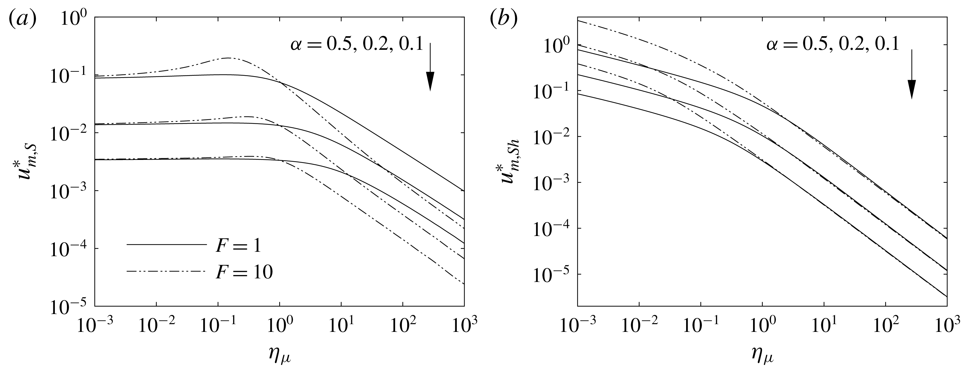
(2.22) $$\begin{eqnarray}\displaystyle & \displaystyle u_{m,S}^{\ast }={\displaystyle \frac{\displaystyle \int _{0}^{\unicode[STIX]{x1D714}}\!\!\displaystyle \int _{0}^{\unicode[STIX]{x1D6FC}}u^{\ast }\,\text{d}y^{\ast }\,\text{d}z^{\ast }}{\displaystyle \int _{0}^{\unicode[STIX]{x1D714}}\!\!\displaystyle \int _{0}^{\unicode[STIX]{x1D6FC}}\,\text{d}y^{\ast }\,\text{d}z^{\ast }}}={\displaystyle \frac{\displaystyle \int _{0}^{\unicode[STIX]{x1D714}}\!\!\displaystyle \int _{0}^{\unicode[STIX]{x1D6FC}}\!u^{\ast }\,\text{d}y^{\ast }\,\text{d}z^{\ast }}{\unicode[STIX]{x1D714}\unicode[STIX]{x1D6FC}}}=\mathop{\sum }_{j=1}^{N}{\displaystyle \frac{d_{j}(-1)^{l_{j}}\sin (\unicode[STIX]{x1D709}_{m_{j}}\unicode[STIX]{x1D714})}{\unicode[STIX]{x1D714}\unicode[STIX]{x1D709}_{l_{j}}\unicode[STIX]{x1D709}_{m_{j}}}}, & \displaystyle\end{eqnarray}$$

(2.23) $$\begin{eqnarray}\displaystyle & \displaystyle u_{m,Sh}^{\ast }={\displaystyle \frac{\displaystyle \int _{\unicode[STIX]{x1D714}}^{1}\!\!\displaystyle \int _{0}^{\unicode[STIX]{x1D6FC}}\!u^{\ast }\,\text{d}y^{\ast }\,\text{d}z^{\ast }}{\displaystyle \int _{\unicode[STIX]{x1D714}}^{1}\!\!\displaystyle \int _{0}^{\unicode[STIX]{x1D6FC}}\,\text{d}y^{\ast }\,\text{d}z^{\ast }}}={\displaystyle \frac{\displaystyle \int _{\unicode[STIX]{x1D714}}^{1}\!\!\displaystyle \int _{0}^{\unicode[STIX]{x1D6FC}}\!u^{\ast }\,\text{d}y^{\ast }\,\text{d}z^{\ast }}{(1-\unicode[STIX]{x1D714})\unicode[STIX]{x1D6FC}}}=\mathop{\sum }_{j=1}^{N}{\displaystyle \frac{d_{j}(-1)^{l_{j}}[(-1)^{m_{j}}-\sin (\unicode[STIX]{x1D709}_{m_{j}}\unicode[STIX]{x1D714})]}{(1-\unicode[STIX]{x1D714})\unicode[STIX]{x1D709}_{l_{j}}\unicode[STIX]{x1D709}_{m_{j}}}},\qquad \,\,\, & \displaystyle\end{eqnarray}$$

(2.24) $$\begin{eqnarray}\displaystyle & \displaystyle u_{m}^{\ast }={\displaystyle \frac{\displaystyle \int _{0}^{1}\!\!\displaystyle \int _{0}^{\unicode[STIX]{x1D6FC}}\!u^{\ast }\,\text{d}y^{\ast }\,\text{d}z^{\ast }}{\displaystyle \int _{0}^{1}\!\!\displaystyle \int _{0}^{\unicode[STIX]{x1D6FC}}\,\text{d}y^{\ast }\,\text{d}z^{\ast }}}=\unicode[STIX]{x1D714}u_{m,S}^{\ast }+(1-\unicode[STIX]{x1D714})u_{m,Sh}^{\ast }=\mathop{\sum }_{j=1}^{N}{\displaystyle \frac{d_{j}(-1)^{l_{j}+m_{j}}}{\unicode[STIX]{x1D709}_{l_{j}}\unicode[STIX]{x1D709}_{m_{j}}}}. & \displaystyle\end{eqnarray}$$

As shown, $u_{m,S}^{\ast }$ and $u_{m,Sh}^{\ast }$ and, consequently, $\unicode[STIX]{x1D6E4}$ are functions of $\unicode[STIX]{x1D714}$ in terms of infinite series. Accordingly, solving (2.21) for $\unicode[STIX]{x1D714}$ is not directly possible and a trial and error analysis should be performed. The iterative method used here starts by making an initial guess for $\unicode[STIX]{x1D6E4}$ based on which $\unicode[STIX]{x1D714}$ is obtained from (2.21) for a given $F$ . The predicted value of $\unicode[STIX]{x1D714}$ is then used to determine the flow field at given values of $\unicode[STIX]{x1D6FC}$ and $\unicode[STIX]{x1D702}_{\unicode[STIX]{x1D707}}$ . The values of $u_{m,S}^{\ast }$ and $u_{m,Sh}^{\ast }$ are then calculated from (2.22) and (2.23) to update $\unicode[STIX]{x1D6E4}$ and the next round of iteration starts after applying an appropriate under relaxation factor. The iterations continue until the relative difference between two successive estimations of $\unicode[STIX]{x1D714}$ becomes less than $10^{-5}$ . The number of iterations required depends on both the number of terms included in the series and the flow parameters. However, less than 15 iterations are needed to get converged results in most cases, indicating the superiority of the model presented over standard numerical methods in terms of the computational cost.

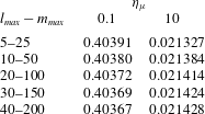
To achieve a view of the number of the series terms required to obtain accurate results, a convergence analysis is made in table 2. It can be seen that even by setting $l_{max}=10$ and $m_{max}=50$ reasonably accurate results are achieved so that the maximum relative difference between the calculated values of $u_{m}^{\ast }$ for this case and those of $l_{max}=40$ and $m_{max}=200$ is only approximately 0.2 %. Hence, the latter set is considered for presentation of the hydrodynamic features and the former set is used for evaluation of the mass transport characteristics that require more computationally expensive procedures.

Table 2.

Values of $u_{m}^{\ast }$ calculated using different numbers of terms included in the series at two different values of $\unicode[STIX]{x1D702}_{\unicode[STIX]{x1D707}}$ while keeping $\unicode[STIX]{x1D6FC}=F=1$ .

Before proceeding further, it is emphasized that, although $\unicode[STIX]{x2202}p/\unicode[STIX]{x2202}x$ is used for scaling of the fluid velocity, the determination of the axial pressure gradient is not necessary for evaluation of the dimensional velocity. In fact, the ratio $u/u_{m}=u^{\ast }/u_{m}^{\ast }$ is known at any point once the problem is solved and the overall mean velocity in the channel is readily obtained as $u_{m}=(Q_{S}+Q_{Sh})/4WH$ since the sample and sheath flow rates are specified. Accordingly, the dimensional velocity may be obtained as $u=(u^{\ast }/u_{m}^{\ast })[(Q_{S}+Q_{Sh})/4WH]$ .

2.2.2 Single-phase flow solution

For $\unicode[STIX]{x1D702}_{\unicode[STIX]{x1D707}}=1$ , corresponding to a single-phase flow, the elements of $\unicode[STIX]{x1D63D}$ reduce to $b_{ij}=0$ for $i\neq j$ and

(2.25) $$\begin{eqnarray}b_{ii}={\displaystyle \frac{\unicode[STIX]{x1D6FC}\unicode[STIX]{x1D709}_{m_{i}}^{2}}{4}}+{\displaystyle \frac{\unicode[STIX]{x1D709}_{l_{i}}^{2}}{4\unicode[STIX]{x1D6FC}}}.\end{eqnarray}$$

Therefore, the coefficients $d_{i}$ are easily obtained from (2.13) as

(2.26) $$\begin{eqnarray}d_{i}={\displaystyle \frac{e_{i}}{b_{ii}}}={\displaystyle \frac{4\unicode[STIX]{x1D6FC}^{2}(-1)^{l_{i}+m_{i}}}{\unicode[STIX]{x1D709}_{m_{i}}\unicode[STIX]{x1D709}_{l_{i}}^{3}+\unicode[STIX]{x1D6FC}^{2}\unicode[STIX]{x1D709}_{l_{i}}\unicode[STIX]{x1D709}_{m_{i}}^{3}}}.\end{eqnarray}$$

2.2.3 Limiting case for large aspect ratio ( $1\ll H/W$ )

When $1\ll \unicode[STIX]{x1D6FC}$ , the problem is significantly simplified because the $y$ -dependence of the results vanishes. Even though this situation is usually not observed in microfluidic instruments because of the pertinent shallow geometries, it has applications in the extrusion of multilayer polymer melts (Williams Reference Williams1975). Moreover, the corresponding solution may serve as a benchmark for validation of the general analysis in the limit $\unicode[STIX]{x1D6FC}\rightarrow \infty$ . As $\unicode[STIX]{x1D6FC}\rightarrow \infty$ , the momentum equation (2.2) is solved subject to boundary and interfacial conditions instead of utilizing the single-domain formulation. Discarding the derivative with respect to $y$ in (2.2), the following equations may be obtained for the sample and sheath flows, respectively,

(2.27) $$\begin{eqnarray}\displaystyle & \displaystyle {\displaystyle \frac{\text{d}^{2}u_{S}^{\ast }}{\text{d}z^{\ast 2}}}+1=0, & \displaystyle\end{eqnarray}$$

(2.28) $$\begin{eqnarray}\displaystyle & \displaystyle \unicode[STIX]{x1D702}_{\unicode[STIX]{x1D707}}{\displaystyle \frac{\text{d}^{2}u_{Sh}^{\ast }}{\text{d}z^{\ast 2}}}+1=0. & \displaystyle\end{eqnarray}$$

The momentum equations (2.27) and (2.28) are constrained by the following boundary and interfacial conditions

(2.29a-c ) $$\begin{eqnarray}\left.{\displaystyle \frac{\text{d}u_{S}^{\ast }}{\text{d}z^{\ast }}}\right|_{z^{\ast }=0}=u_{Sh}^{\ast }|_{z^{\ast }=1}=0,\quad u_{S}^{\ast }|_{z^{\ast }=\unicode[STIX]{x1D714}}=u_{Sh}^{\ast }|_{z^{\ast }=\unicode[STIX]{x1D714}},\quad \left.{\displaystyle \frac{\text{d}u_{S}^{\ast }}{\text{d}z^{\ast }}}\right|_{z^{\ast }=\unicode[STIX]{x1D714}}=\unicode[STIX]{x1D702}_{\unicode[STIX]{x1D707}}\left.{\displaystyle \frac{\text{d}u_{Sh}^{\ast }}{\text{d}z^{\ast }}}\right|_{z^{\ast }=\unicode[STIX]{x1D714}}.\end{eqnarray}$$

The last two conditions in (2.29) designate the continuity of the velocity and the shear stress at the sample–sheath interface. It can be easily verified that the solutions of (2.27) and (2.28) subject to boundary conditions (2.29) are given as

(2.30) $$\begin{eqnarray}\displaystyle & \displaystyle u_{S}^{\ast }={\displaystyle \frac{1}{2}}\left(\unicode[STIX]{x1D714}^{2}-z^{\ast 2}\right)+{\displaystyle \frac{1}{2\unicode[STIX]{x1D702}_{\unicode[STIX]{x1D707}}}}(1-\unicode[STIX]{x1D714}^{2}), & \displaystyle\end{eqnarray}$$

(2.31) $$\begin{eqnarray}\displaystyle & \displaystyle u_{Sh}^{\ast }={\displaystyle \frac{1}{2\unicode[STIX]{x1D702}_{\unicode[STIX]{x1D707}}}}\left(1-z^{\ast 2}\right). & \displaystyle\end{eqnarray}$$

Furthermore, the dimensionless mean velocities of the sample and sheath streams are obtained as below

(2.32) $$\begin{eqnarray}\displaystyle & \displaystyle u_{m,S}^{\ast }={\displaystyle \frac{\displaystyle \int _{0}^{\unicode[STIX]{x1D714}}u_{S}^{\ast }\,\text{d}z^{\ast }}{\unicode[STIX]{x1D714}}}={\displaystyle \frac{\unicode[STIX]{x1D714}^{2}}{3}}+{\displaystyle \frac{1}{2\unicode[STIX]{x1D702}_{\unicode[STIX]{x1D707}}}}(1-\unicode[STIX]{x1D714}^{2}), & \displaystyle\end{eqnarray}$$

(2.33) $$\begin{eqnarray}\displaystyle & \displaystyle u_{m,Sh}^{\ast }={\displaystyle \frac{\displaystyle \int _{\unicode[STIX]{x1D714}}^{1}u_{Sh}^{\ast }\,\text{d}z^{\ast }}{1-\unicode[STIX]{x1D714}}}={\displaystyle \frac{1}{6\unicode[STIX]{x1D702}_{\unicode[STIX]{x1D707}}}}(2-\unicode[STIX]{x1D714}-\unicode[STIX]{x1D714}^{2}). & \displaystyle\end{eqnarray}$$

In addition, from (2.32) and (2.33), the dimensionless overall mean velocity is calculated as

(2.34) $$\begin{eqnarray}u_{m}^{\ast }=\unicode[STIX]{x1D714}u_{m,S}^{\ast }+(1-\unicode[STIX]{x1D714})u_{m,Sh}^{\ast }={\displaystyle \frac{\unicode[STIX]{x1D714}^{3}}{3}}+{\displaystyle \frac{1}{3\unicode[STIX]{x1D702}_{\unicode[STIX]{x1D707}}}}(1-\unicode[STIX]{x1D714}^{3}).\end{eqnarray}$$

As before, an iterative approach is utilized to determine $\unicode[STIX]{x1D714}$ using (2.21), (2.32), and (2.33).

2.2.4 Limiting case for small aspect ratio ( $H/W\ll 1$ )

The situation where the channel height is considerably smaller than the width is frequently encountered in microfluidics devices. In these cases, for which $\unicode[STIX]{x1D6FC}\ll 1$ , the $z$ -dependence of the velocity distribution vanishes except over small regions at the boundaries and the interfaces. Neglecting these regions, the momentum equation takes the following forms for the sample and sheath flows, respectively,

(2.35) $$\begin{eqnarray}\displaystyle & \displaystyle {\displaystyle \frac{\text{d}^{2}u_{S}^{\ast }}{\text{d}y^{\ast ^{2}}}}+1=0, & \displaystyle\end{eqnarray}$$

(2.36) $$\begin{eqnarray}\displaystyle & \displaystyle \unicode[STIX]{x1D702}_{\unicode[STIX]{x1D707}}{\displaystyle \frac{\text{d}^{2}u_{Sh}^{\ast }}{\text{d}y^{\ast ^{2}}}}+1=0, & \displaystyle\end{eqnarray}$$

which, upon applying the symmetry and no-slip boundary conditions, provide

(2.37) $$\begin{eqnarray}\displaystyle & \displaystyle u_{S}^{\ast }={\displaystyle \frac{\unicode[STIX]{x1D6FC}^{2}-y^{\ast ^{2}}}{2}}, & \displaystyle\end{eqnarray}$$

(2.38) $$\begin{eqnarray}\displaystyle & \displaystyle u_{Sh}^{\ast }={\displaystyle \frac{\unicode[STIX]{x1D6FC}^{2}-y^{\ast ^{2}}}{2\unicode[STIX]{x1D702}_{\unicode[STIX]{x1D707}}}}. & \displaystyle\end{eqnarray}$$

In this case, the dimensionless mean velocities of the sample and sheath flows are obtained as

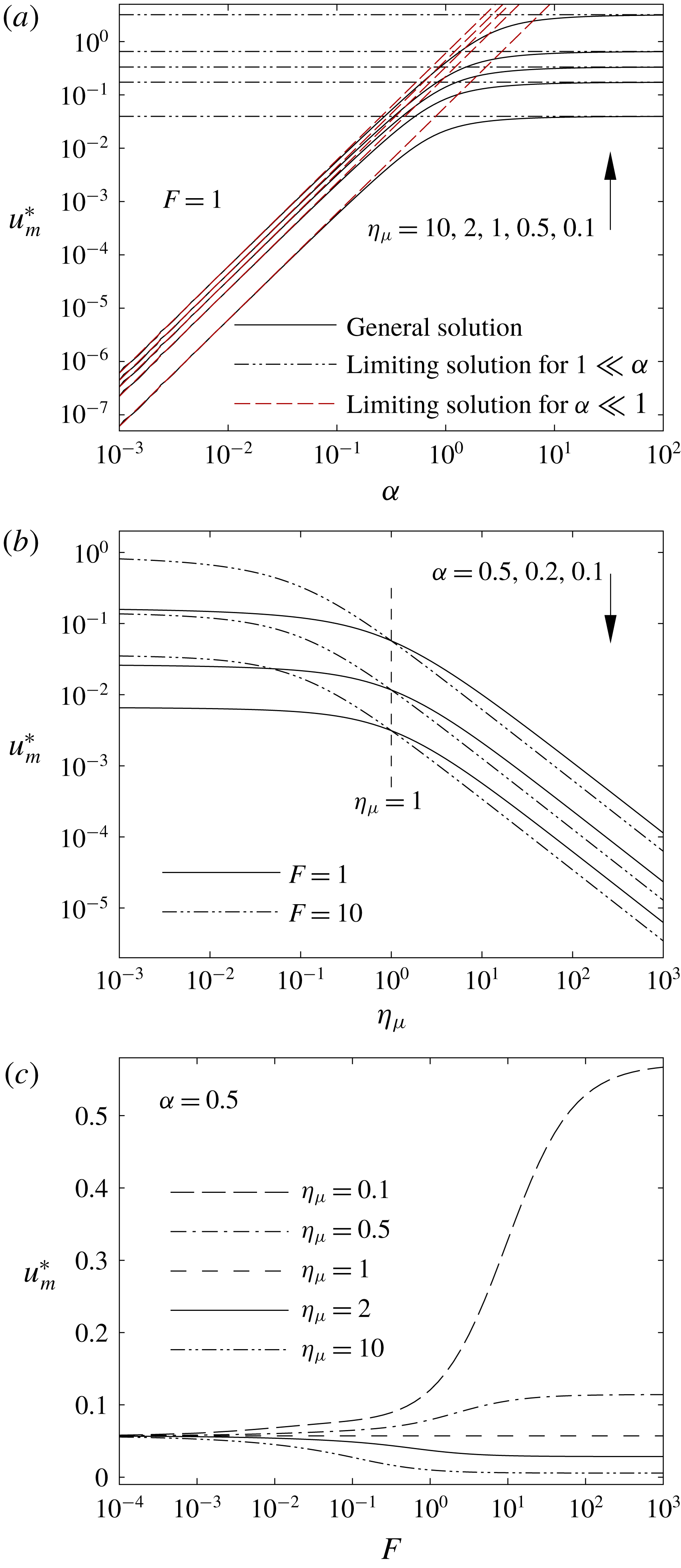
(2.39) $$\begin{eqnarray}\displaystyle & \displaystyle u_{m,S}^{\ast }={\displaystyle \frac{\displaystyle \int _{0}^{\unicode[STIX]{x1D6FC}}u_{S}^{\ast }\,\text{d}y^{\ast }}{\unicode[STIX]{x1D6FC}}}={\displaystyle \frac{\unicode[STIX]{x1D6FC}^{2}}{3}}, & \displaystyle\end{eqnarray}$$

(2.40) $$\begin{eqnarray}\displaystyle & \displaystyle u_{m,Sh}^{\ast }={\displaystyle \frac{\displaystyle \int _{0}^{\unicode[STIX]{x1D6FC}}u_{Sh}^{\ast }\,\text{d}y^{\ast }}{\unicode[STIX]{x1D6FC}}}={\displaystyle \frac{\unicode[STIX]{x1D6FC}^{2}}{3\unicode[STIX]{x1D702}_{\unicode[STIX]{x1D707}}}}. & \displaystyle\end{eqnarray}$$

Hence, the mean velocity ratio becomes $\unicode[STIX]{x1D6E4}=\unicode[STIX]{x1D702}_{\unicode[STIX]{x1D707}}^{-1}$ , leading to the following expression for the dimensionless focusing width

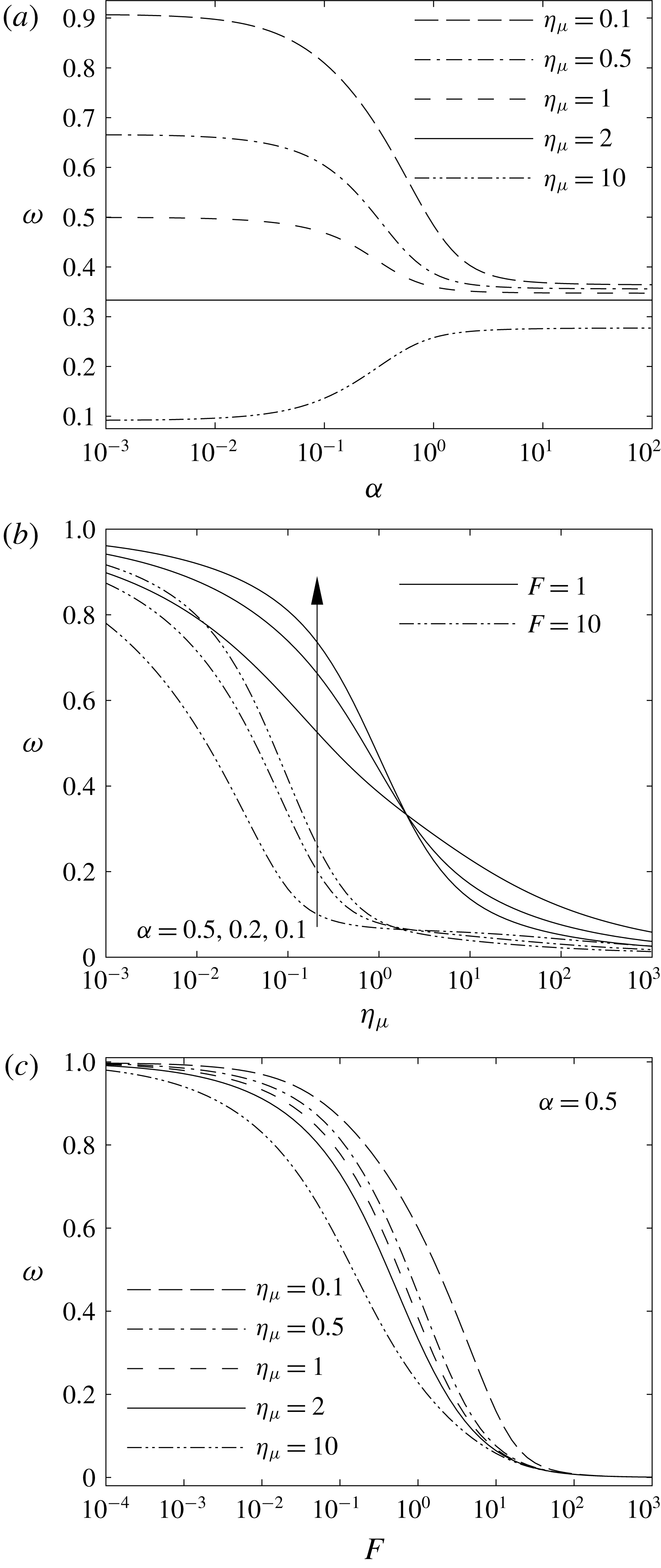
(2.41) $$\begin{eqnarray}\unicode[STIX]{x1D714}={\displaystyle \frac{1}{1+F\unicode[STIX]{x1D702}_{\unicode[STIX]{x1D707}}}}.\end{eqnarray}$$

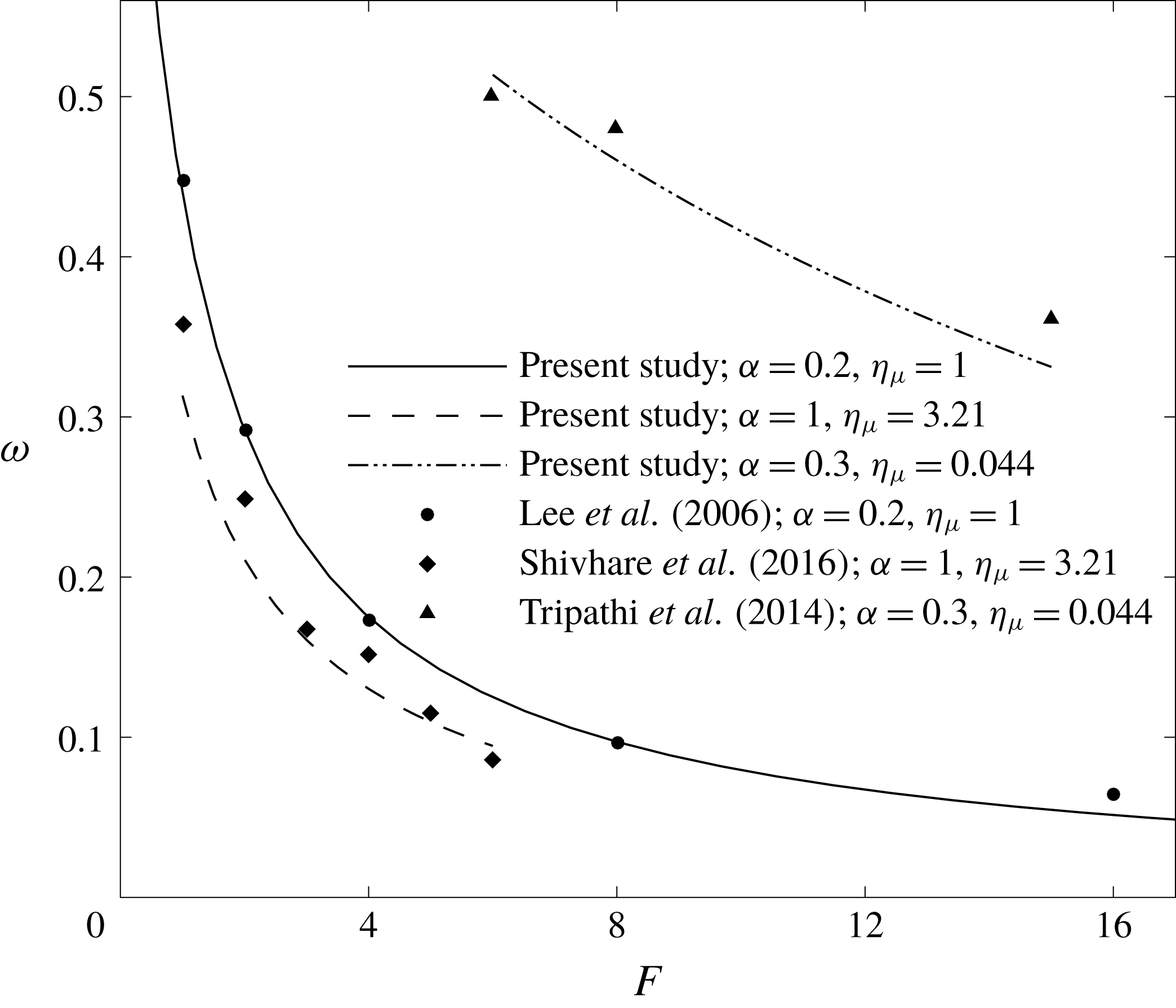
Equation (2.42) is the same as the expression derived by Tripathi et al. (Reference Tripathi, Chakravarty and Agrawal2014) for $\unicode[STIX]{x1D6FC}\ll 1$ . Finally, using the expression for $\unicode[STIX]{x1D714}$ , given by (2.41), the overall dimensionless mean velocity may be obtained as

(2.42) $$\begin{eqnarray}u_{m}^{\ast }=\unicode[STIX]{x1D714}u_{m,S}^{\ast }+(1-\unicode[STIX]{x1D714})u_{m,Sh}^{\ast }={\displaystyle \frac{\unicode[STIX]{x1D6FC}^{2}}{3}}{\displaystyle \frac{1+F}{1+F\unicode[STIX]{x1D702}_{\unicode[STIX]{x1D707}}}}.\end{eqnarray}$$

2.3 Concentration distribution

2.3.1 General solution

In the single-domain formulation, the species conservation equation is given by

(2.43) $$\begin{eqnarray}u{\displaystyle \frac{\unicode[STIX]{x2202}c}{\unicode[STIX]{x2202}x}}=D{\displaystyle \frac{\unicode[STIX]{x2202}^{2}c}{\unicode[STIX]{x2202}x^{2}}}+{\displaystyle \frac{\unicode[STIX]{x2202}}{\unicode[STIX]{x2202}y}}\left(D{\displaystyle \frac{\unicode[STIX]{x2202}c}{\unicode[STIX]{x2202}y}}\right)+{\displaystyle \frac{\unicode[STIX]{x2202}}{\unicode[STIX]{x2202}z}}\left(D{\displaystyle \frac{\unicode[STIX]{x2202}c}{\unicode[STIX]{x2202}z}}\right),\end{eqnarray}$$

where $c$ denotes the number concentration and $D$ represents the molecular diffusivity. Although our formulation is sufficiently general that we may specify any cross-sectional distribution of $D$ , here we consider $D$ to be constant within each phase with a possible change from $D_{S}$ to $D_{Sh}$ at the sample–sheath interface. The dimensionless form of (2.43) may be written as

(2.44) $$\begin{eqnarray}{\displaystyle \frac{u^{\ast }}{u_{m}^{\ast }}}{\displaystyle \frac{\unicode[STIX]{x2202}c^{\ast }}{\unicode[STIX]{x2202}x^{\ast }}}={\displaystyle \frac{D^{\ast }}{Pe^{2}}}{\displaystyle \frac{\unicode[STIX]{x2202}^{2}c^{\ast }}{\unicode[STIX]{x2202}x^{\ast 2}}}+{\displaystyle \frac{\unicode[STIX]{x2202}}{\unicode[STIX]{x2202}y^{\ast }}}\left(D^{\ast }{\displaystyle \frac{\unicode[STIX]{x2202}c^{\ast }}{\unicode[STIX]{x2202}y^{\ast }}}\right)+{\displaystyle \frac{\unicode[STIX]{x2202}}{\unicode[STIX]{x2202}z^{\ast }}}\left(D^{\ast }{\displaystyle \frac{\unicode[STIX]{x2202}c^{\ast }}{\unicode[STIX]{x2202}z^{\ast }}}\right),\end{eqnarray}$$

where $D^{\ast }=D/D_{S}$ and $c^{\ast }=c/c_{0}$ . In addition, $x^{\ast }=x/WPe$ with $Pe=u_{m}W/D_{S}$ being the Péclet number. The corresponding boundary conditions for (2.44) include

(2.45) $$\begin{eqnarray}\displaystyle & \displaystyle \left.{\displaystyle \frac{\unicode[STIX]{x2202}c^{\ast }}{\unicode[STIX]{x2202}y^{\ast }}}\right|_{y^{\ast }=0,\unicode[STIX]{x1D6FC}}=\left.{\displaystyle \frac{\unicode[STIX]{x2202}c^{\ast }}{\unicode[STIX]{x2202}z^{\ast }}}\right|_{z^{\ast }=\pm 1}=0, & \displaystyle\end{eqnarray}$$

(2.46) $$\begin{eqnarray}\displaystyle & \displaystyle \left.c^{\ast }\right|_{x^{\ast }=0}=\left\{\begin{array}{@{}ll@{}}0,\quad & -1\leqslant z^{\ast }<-\unicode[STIX]{x1D714}\\ 1,\quad & -\unicode[STIX]{x1D714}<z^{\ast }<\unicode[STIX]{x1D714}\\ 0,\quad & \unicode[STIX]{x1D714}<z^{\ast }\leqslant 1.\end{array}\right. & \displaystyle\end{eqnarray}$$

It should be pointed out that in (2.45) we apply the no-flux condition at $z^{\ast }=-1$ instead of utilizing the symmetry at $z^{\ast }=0$ for the sake of generality. This way, the majority of the analysis remains unchanged for any distribution of the inlet concentration along the channel width. The general solution of the dimensionless species conservation equation will contain the terms $\text{e}^{-\unicode[STIX]{x1D6FD}_{n}^{2}x^{\ast }}$ and $\text{e}^{\unicode[STIX]{x1D6FD}_{n}^{2}x^{\ast }}$ , wherein $\unicode[STIX]{x1D6FD}_{n}^{2}$ is a positive real eigenvalue. Since the solution should satisfy the condition of a bounded concentration at $x^{\ast }\rightarrow \infty$ , the exponential term of positive argument is not acceptable. The concentration distribution, hence, becomes

(2.47) $$\begin{eqnarray}c^{\ast }=\mathop{\sum }_{n=1}^{\infty }A_{n}G_{n}\left(y^{\ast },z^{\ast }\right)\text{e}^{-\unicode[STIX]{x1D6FD}_{n}^{2}x^{\ast }},\end{eqnarray}$$

where $G_{n}(y^{\ast },z^{\ast })$ is the eigenfunction associated with $\unicode[STIX]{x1D6FD}_{n}^{2}$ and $A_{n}$ is a constant coefficient. Substituting (2.47) into (2.44) and (2.45), gives the following problem for $G_{n}$ :

(2.48) $$\begin{eqnarray}\displaystyle & \displaystyle {\displaystyle \frac{\unicode[STIX]{x2202}}{\unicode[STIX]{x2202}y^{\ast }}}\left(D^{\ast }{\displaystyle \frac{\unicode[STIX]{x2202}G_{n}}{\unicode[STIX]{x2202}y^{\ast }}}\right)+{\displaystyle \frac{\unicode[STIX]{x2202}}{\unicode[STIX]{x2202}z^{\ast }}}\left(D^{\ast }{\displaystyle \frac{\unicode[STIX]{x2202}G_{n}}{\unicode[STIX]{x2202}z^{\ast }}}\right)+\unicode[STIX]{x1D6FD}_{n}^{2}\left({\displaystyle \frac{D^{\ast }\unicode[STIX]{x1D6FD}_{n}^{2}}{Pe^{2}}}+{\displaystyle \frac{u^{\ast }}{u_{m}^{\ast }}}\right)G_{n}=0, & \displaystyle\end{eqnarray}$$

(2.49) $$\begin{eqnarray}\displaystyle & \displaystyle \left.{\displaystyle \frac{\unicode[STIX]{x2202}G_{n}}{\unicode[STIX]{x2202}y^{\ast }}}\right|_{y^{\ast }=0,\unicode[STIX]{x1D6FC}}=\left.{\displaystyle \frac{\unicode[STIX]{x2202}G_{n}}{\unicode[STIX]{x2202}z^{\ast }}}\right|_{z^{\ast }=\pm 1}=0. & \displaystyle\end{eqnarray}$$

As before, variational calculus is utilized to solve (2.48) and (2.49). The appropriate functional is given as

(2.50) $$\begin{eqnarray}\displaystyle & & \displaystyle \displaystyle I_{G}=\displaystyle \int _{\mathbb{A}^{\ast }}\left\{D^{\ast }\left({\displaystyle \frac{\unicode[STIX]{x2202}G_{n}}{\unicode[STIX]{x2202}y^{\ast }}}\right)^{2}+D^{\ast }\left({\displaystyle \frac{\unicode[STIX]{x2202}G_{n}}{\unicode[STIX]{x2202}z^{\ast }}}\right)^{2}-\unicode[STIX]{x1D6FD}_{n}^{2}\left({\displaystyle \frac{D^{\ast }\unicode[STIX]{x1D6FD}_{n}^{2}}{Pe^{2}}}+{\displaystyle \frac{u^{\ast }}{u_{m}^{\ast }}}\right)G_{n}^{2}\right.\nonumber\\ \displaystyle & & \displaystyle \qquad \left.-\,{\displaystyle \frac{1}{2}}\left[{\displaystyle \frac{\unicode[STIX]{x2202}}{\unicode[STIX]{x2202}y^{\ast }}}\left(D^{\ast }{\displaystyle \frac{\unicode[STIX]{x2202}G_{n}^{2}}{\unicode[STIX]{x2202}y^{\ast }}}\right)+{\displaystyle \frac{\unicode[STIX]{x2202}}{\unicode[STIX]{x2202}z^{\ast }}}\left(D^{\ast }{\displaystyle \frac{\unicode[STIX]{x2202}G_{n}^{2}}{\unicode[STIX]{x2202}z^{\ast }}}\right)\right]\!\right\}\text{d}\mathbb{A}^{\ast }.\end{eqnarray}$$

Moreover, $G_{n}$ is considered to be

(2.51) $$\begin{eqnarray}G_{n}=\mathop{\sum }_{j=1}^{M}t_{nj}g_{j},\end{eqnarray}$$

wherein the basis functions are of the form

(2.52) $$\begin{eqnarray}g_{j}(y^{\ast },z^{\ast })=\cos (\unicode[STIX]{x1D709}_{q_{j}}y^{\ast }/\unicode[STIX]{x1D6FC})\cos [\unicode[STIX]{x1D709}_{r_{j}}(z^{\ast }+1)],\end{eqnarray}$$

where $\unicode[STIX]{x1D709}_{q_{j}}=q_{j}\unicode[STIX]{x03C0}$ and $\unicode[STIX]{x1D709}_{r_{j}}=r_{j}\unicode[STIX]{x03C0}/2$ with $q_{j}=0,1,2,\ldots ,q_{max}$ , $r_{j}=0,1,2,\ldots ,r_{max}$ , and $M=(q_{max}+1)(r_{max}+1)$ . We set $q_{max}=10$ and $r_{max}=300$ so that $M=3311$ . The minimization of $I_{G}(t_{n1},t_{n2},\ldots ,t_{nM})$ leads to the following set of equations:

(2.53) $$\begin{eqnarray}\displaystyle & & \displaystyle 2\displaystyle \int _{\mathbb{A}^{\ast }}\left[D^{\ast }{\displaystyle \frac{\unicode[STIX]{x2202}G_{n}}{\unicode[STIX]{x2202}y^{\ast }}}{\displaystyle \frac{\unicode[STIX]{x2202}g_{i}}{\unicode[STIX]{x2202}y^{\ast }}}+D^{\ast }{\displaystyle \frac{\unicode[STIX]{x2202}G_{n}}{\unicode[STIX]{x2202}z^{\ast }}}{\displaystyle \frac{\unicode[STIX]{x2202}g_{i}}{\unicode[STIX]{x2202}z^{\ast }}}-\unicode[STIX]{x1D6FD}_{n}^{2}\left({\displaystyle \frac{D^{\ast }\unicode[STIX]{x1D6FD}_{n}^{2}}{Pe^{2}}}+{\displaystyle \frac{u^{\ast }}{u_{m}^{\ast }}}\right)G_{n}g_{i}\right]\text{d}\mathbb{A}^{\ast }\nonumber\\ \displaystyle & & \displaystyle \quad -\,\displaystyle \int _{\mathbb{A}^{\ast }}\left\{{\displaystyle \frac{\unicode[STIX]{x2202}}{\unicode[STIX]{x2202}y^{\ast }}}\left[D^{\ast }{\displaystyle \frac{\unicode[STIX]{x2202}\left(G_{n}g_{i}\right)}{\unicode[STIX]{x2202}y^{\ast }}}\right]+{\displaystyle \frac{\unicode[STIX]{x2202}}{\unicode[STIX]{x2202}z^{\ast }}}\left[D^{\ast }{\displaystyle \frac{\unicode[STIX]{x2202}\left(G_{n}g_{i}\right)}{\unicode[STIX]{x2202}z^{\ast }}}\right]\!\right\}\text{d}\mathbb{A}^{\ast }=0\nonumber\\ \displaystyle & & \displaystyle \qquad \text{for }i=1,2,\ldots ,M.\end{eqnarray}$$

Similar to that of the velocity distribution, the second integral in (2.53) vanishes because of the boundary conditions. Hence, after substitution for $G_{n}$ from (2.51) into (2.53), it evolves into

(2.54) $$\begin{eqnarray}\displaystyle & & \displaystyle \mathop{\sum }_{j=1}^{M}t_{nj}\left[\displaystyle \int _{\mathbb{A}^{\ast }}\left(D^{\ast }{\displaystyle \frac{\unicode[STIX]{x2202}g_{i}}{\unicode[STIX]{x2202}y^{\ast }}}{\displaystyle \frac{\unicode[STIX]{x2202}g_{j}}{\unicode[STIX]{x2202}y^{\ast }}}+D^{\ast }{\displaystyle \frac{\unicode[STIX]{x2202}g_{i}}{\unicode[STIX]{x2202}z^{\ast }}}{\displaystyle \frac{\unicode[STIX]{x2202}g_{j}}{\unicode[STIX]{x2202}z^{\ast }}}\right)\text{d}\mathbb{A}^{\ast }\right.\nonumber\\ \displaystyle & & \displaystyle \left.\quad -\,{\displaystyle \frac{\unicode[STIX]{x1D6FD}_{n}^{2}}{u_{m}^{\ast }}}\displaystyle \int _{\mathbb{A}^{\ast }}u^{\ast }g_{i}g_{j}\text{d}\mathbb{A}^{\ast }-{\displaystyle \frac{\unicode[STIX]{x1D6FD}_{n}^{4}}{Pe^{2}}}\displaystyle \int _{\mathbb{A}^{\ast }}D^{\ast }g_{i}g_{j}\,\text{d}\mathbb{A}^{\ast }\right]=0\quad \text{for }i=1,2,\ldots ,M,\qquad\end{eqnarray}$$

which is a system of $M$ equations of $M+1$ unknowns including $t_{n1},t_{n2},\ldots ,t_{nM}$ , and $\unicode[STIX]{x1D6FD}_{n}^{2}$ and may be written in a compact form as

(2.55) $$\begin{eqnarray}(\unicode[STIX]{x1D643}+\unicode[STIX]{x1D6FD}^{2}\unicode[STIX]{x1D64B}+\unicode[STIX]{x1D6FD}^{4}\unicode[STIX]{x1D64E})\boldsymbol{t}=0,\end{eqnarray}$$

wherein vector $\boldsymbol{t}$ stands for the coefficients $t_{n1},t_{n2},\ldots ,t_{nM}$ and $\unicode[STIX]{x1D643}$ , $\unicode[STIX]{x1D64B}$ , and $\unicode[STIX]{x1D64E}$ are symmetric matrices with the following elements

(2.56) $$\begin{eqnarray}\displaystyle & \displaystyle h_{ij}=\displaystyle \int _{\mathbb{A}^{\ast }}\left(D^{\ast }{\displaystyle \frac{\unicode[STIX]{x2202}g_{i}}{\unicode[STIX]{x2202}y^{\ast }}}{\displaystyle \frac{\unicode[STIX]{x2202}g_{j}}{\unicode[STIX]{x2202}y^{\ast }}}+D^{\ast }{\displaystyle \frac{\unicode[STIX]{x2202}g_{i}}{\unicode[STIX]{x2202}z^{\ast }}}{\displaystyle \frac{\unicode[STIX]{x2202}g_{j}}{\unicode[STIX]{x2202}z^{\ast }}}\right)\text{d}\mathbb{A}^{\ast }, & \displaystyle\end{eqnarray}$$

(2.57) $$\begin{eqnarray}\displaystyle & \displaystyle p_{ij}=-{\displaystyle \frac{1}{u_{m}^{\ast }}}\displaystyle \int _{\mathbb{A}^{\ast }}u^{\ast }g_{i}g_{j}\,\text{d}\mathbb{A}^{\ast }, & \displaystyle\end{eqnarray}$$

(2.58) $$\begin{eqnarray}\displaystyle & \displaystyle s_{ij}=-\displaystyle \int _{\mathbb{A}^{\ast }}{\displaystyle \frac{D^{\ast }g_{i}g_{j}}{Pe^{2}}}\,\text{d}\mathbb{A}^{\ast }. & \displaystyle\end{eqnarray}$$

Substituting $u^{\ast }$ and $g$ from (2.8) and (2.52), respectively, and recalling that $D^{\ast }=1$ in $\mathbb{A}_{S}^{\ast }$ and $D^{\ast }=D_{Sh}/D_{S}=\unicode[STIX]{x1D702}_{D}$ in $\mathbb{A}_{Sh}^{\ast }$ , it can be shown that

(2.59) $$\begin{eqnarray}\displaystyle h_{ij} & = & \displaystyle {\displaystyle \frac{\unicode[STIX]{x1D709}_{q_{i}}\unicode[STIX]{x1D709}_{q_{j}}\unicode[STIX]{x1D6FF}_{q_{i},q_{j}}}{2\unicode[STIX]{x1D6FC}}}\left\{\vphantom{{\displaystyle \frac{\int }{\int }}}2[\unicode[STIX]{x1D702}_{D}+\unicode[STIX]{x1D714}(1-\unicode[STIX]{x1D702}_{D})]\unicode[STIX]{x1D6FF}_{0,r_{i}+r_{j}}\right.\nonumber\\ \displaystyle & & \displaystyle +\,\unicode[STIX]{x1D6FF}_{r_{i},r_{j}}(1-\unicode[STIX]{x1D6FF}_{0,r_{i}+r_{j}})\left[\unicode[STIX]{x1D702}_{D}+\unicode[STIX]{x1D714}(1-\unicode[STIX]{x1D702}_{D})+{\displaystyle \frac{(1-\unicode[STIX]{x1D702}_{D})(-1)^{r_{i}}}{\unicode[STIX]{x1D709}_{r_{i}}+\unicode[STIX]{x1D709}_{r_{j}}+\unicode[STIX]{x1D6FF}_{0,r_{i}+r_{j}}}}\sin (2\unicode[STIX]{x1D709}_{r_{i}}\unicode[STIX]{x1D714})\right]\nonumber\\ \displaystyle & & \displaystyle +\,(1-\unicode[STIX]{x1D702}_{D})(1-\unicode[STIX]{x1D6FF}_{r_{i},r_{j}})\left\{{\displaystyle \frac{\cos (\unicode[STIX]{x1D709}_{r_{i}}-\unicode[STIX]{x1D709}_{r_{j}})\sin [(\unicode[STIX]{x1D709}_{r_{i}}-\unicode[STIX]{x1D709}_{r_{j}})\unicode[STIX]{x1D714}]}{\unicode[STIX]{x1D709}_{r_{i}}-\unicode[STIX]{x1D709}_{r_{j}}+\unicode[STIX]{x1D6FF}_{r_{i},r_{j}}}}\right.\nonumber\\ \displaystyle & & \displaystyle +\left.\left.{\displaystyle \frac{\cos (\unicode[STIX]{x1D709}_{r_{i}}+\unicode[STIX]{x1D709}_{r_{j}})\sin [(\unicode[STIX]{x1D709}_{r_{i}}+\unicode[STIX]{x1D709}_{r_{j}})\unicode[STIX]{x1D714}]}{\unicode[STIX]{x1D709}_{r_{i}}+\unicode[STIX]{x1D709}_{r_{j}}+\unicode[STIX]{x1D6FF}_{0,r_{i}+r_{j}}}}\right\}\right\}\nonumber\\ \displaystyle & & \displaystyle +\,\unicode[STIX]{x1D6FF}_{q_{i},q_{j}}(1+\unicode[STIX]{x1D6FF}_{0,q_{i}+q_{j}}){\displaystyle \frac{\unicode[STIX]{x1D6FC}\unicode[STIX]{x1D709}_{r_{i}}\unicode[STIX]{x1D709}_{r_{j}}}{2}}\left\{\!\left[\unicode[STIX]{x1D702}_{D}+\unicode[STIX]{x1D714}(1-\unicode[STIX]{x1D702}_{D})+{\displaystyle \frac{(\unicode[STIX]{x1D702}_{D}-1)(-1)^{r_{i}}}{\unicode[STIX]{x1D709}_{r_{i}}+\unicode[STIX]{x1D709}_{r_{j}}+\unicode[STIX]{x1D6FF}_{0,r_{i}+r_{j}}}}\sin (2\unicode[STIX]{x1D709}_{r_{i}}\unicode[STIX]{x1D714})\right]\unicode[STIX]{x1D6FF}_{r_{i},r_{j}}\right.\nonumber\\ \displaystyle & & \displaystyle +\,(1-\unicode[STIX]{x1D702}_{D})(1-\unicode[STIX]{x1D6FF}_{r_{i},r_{j}})\left\{{\displaystyle \frac{\cos (\unicode[STIX]{x1D709}_{r_{i}}-\unicode[STIX]{x1D709}_{r_{j}})\sin [(\unicode[STIX]{x1D709}_{r_{i}}-\unicode[STIX]{x1D709}_{r_{j}})\unicode[STIX]{x1D714}]}{\unicode[STIX]{x1D709}_{r_{i}}-\unicode[STIX]{x1D709}_{r_{j}}+\unicode[STIX]{x1D6FF}_{r_{i},r_{j}}}}\right.\nonumber\\ \displaystyle & & \displaystyle -\left.\left.{\displaystyle \frac{\cos (\unicode[STIX]{x1D709}_{r_{i}}+\unicode[STIX]{x1D709}_{r_{j}})\sin [(\unicode[STIX]{x1D709}_{r_{i}}+\unicode[STIX]{x1D709}_{r_{j}})\unicode[STIX]{x1D714}]}{\unicode[STIX]{x1D709}_{r_{i}}+\unicode[STIX]{x1D709}_{r_{j}}+\unicode[STIX]{x1D6FF}_{0,r_{i}+r_{j}}}}\right\}\right\},\end{eqnarray}$$

(2.60) $$\begin{eqnarray}\displaystyle p_{ij} & = & \displaystyle -{\displaystyle \frac{\unicode[STIX]{x1D6FC}}{16u_{m}^{\ast }}}\mathop{\sum }_{k=1}^{N}d_{k}\left[{\displaystyle \frac{(-1)^{l_{k}-q_{i}+q_{j}}}{\unicode[STIX]{x1D709}_{l_{k}}-\unicode[STIX]{x1D709}_{q_{i}}+\unicode[STIX]{x1D709}_{q_{j}}}}+{\displaystyle \frac{(-1)^{l_{k}+q_{i}-q_{j}}}{\unicode[STIX]{x1D709}_{l_{k}}+\unicode[STIX]{x1D709}_{q_{i}}-\unicode[STIX]{x1D709}_{q_{j}}}}+{\displaystyle \frac{(-1)^{l_{k}-q_{i}-q_{j}}}{\unicode[STIX]{x1D709}_{l_{k}}-\unicode[STIX]{x1D709}_{q_{i}}-\unicode[STIX]{x1D709}_{q_{j}}}}\right.\nonumber\\ \displaystyle & & \displaystyle \left.+\,{\displaystyle \frac{(-1)^{l_{k}+q_{i}+q_{j}}}{\unicode[STIX]{x1D709}_{l_{k}}+\unicode[STIX]{x1D709}_{q_{i}}+\unicode[STIX]{x1D709}_{q_{j}}}}\right]\left[(1-\unicode[STIX]{x1D6FF}_{0,\unicode[STIX]{x1D709}_{m_{k}}-\unicode[STIX]{x1D709}_{r_{i}}+\unicode[STIX]{x1D709}_{r_{j}}}){\displaystyle \frac{(-1)^{m_{k}-r_{i}+r_{j}}+(-1)^{m_{k}}}{\unicode[STIX]{x1D709}_{m_{k}}-\unicode[STIX]{x1D709}_{r_{i}}+\unicode[STIX]{x1D709}_{r_{j}}+\unicode[STIX]{x1D6FF}_{0,\unicode[STIX]{x1D709}_{m_{k}}-\unicode[STIX]{x1D709}_{r_{i}}+\unicode[STIX]{x1D709}_{r_{j}}}}}\right.\nonumber\\ \displaystyle & & \displaystyle +\,(1-\unicode[STIX]{x1D6FF}_{0,\unicode[STIX]{x1D709}_{m_{k}}+\unicode[STIX]{x1D709}_{r_{i}}-\unicode[STIX]{x1D709}_{r_{j}}}){\displaystyle \frac{(-1)^{m_{k}+r_{i}-r_{j}}+(-1)^{m_{k}}}{\unicode[STIX]{x1D709}_{m_{k}}+\unicode[STIX]{x1D709}_{r_{i}}-\unicode[STIX]{x1D709}_{r_{j}}+\unicode[STIX]{x1D6FF}_{0,\unicode[STIX]{x1D709}_{m_{k}}+\unicode[STIX]{x1D709}_{r_{i}}-\unicode[STIX]{x1D709}_{r_{j}}}}}\nonumber\\ \displaystyle & & \displaystyle \left.+\,(1-\unicode[STIX]{x1D6FF}_{0,\unicode[STIX]{x1D709}_{m_{k}}-\unicode[STIX]{x1D709}_{r_{i}}-\unicode[STIX]{x1D709}_{r_{j}}}){\displaystyle \frac{(-1)^{m_{k}-r_{i}-r_{j}}+(-1)^{m_{k}}}{\unicode[STIX]{x1D709}_{m_{k}}-\unicode[STIX]{x1D709}_{r_{i}}-\unicode[STIX]{x1D709}_{r_{j}}+\unicode[STIX]{x1D6FF}_{0,\unicode[STIX]{x1D709}_{m_{k}}-\unicode[STIX]{x1D709}_{r_{i}}-\unicode[STIX]{x1D709}_{r_{j}}}}}+{\displaystyle \frac{(-1)^{m_{k}+r_{i}+r_{j}}+(-1)^{m_{k}}}{\unicode[STIX]{x1D709}_{m_{k}}+\unicode[STIX]{x1D709}_{r_{i}}+\unicode[STIX]{x1D709}_{r_{j}}}}\right],\end{eqnarray}$$

(2.61) $$\begin{eqnarray}\displaystyle s_{ij} & = & \displaystyle \unicode[STIX]{x1D6FF}_{q_{i},q_{j}}(1+\unicode[STIX]{x1D6FF}_{0,q_{i}+q_{j}}){\displaystyle \frac{\unicode[STIX]{x1D6FC}}{2Pe^{2}}}\left\{\vphantom{{\displaystyle \frac{\int }{\int }}}2\left[\unicode[STIX]{x1D714}(\unicode[STIX]{x1D702}_{D}-1)-\unicode[STIX]{x1D702}_{D}\right]\unicode[STIX]{x1D6FF}_{0,r_{i}+r_{j}}\right.\nonumber\\ \displaystyle & & \displaystyle +\,\unicode[STIX]{x1D6FF}_{r_{i},r_{j}}(1-\unicode[STIX]{x1D6FF}_{0,r_{i}+r_{j}})\left[\unicode[STIX]{x1D714}(\unicode[STIX]{x1D702}_{D}-1)-\unicode[STIX]{x1D702}_{D}+{\displaystyle \frac{(\unicode[STIX]{x1D702}_{D}-1)(-1)^{r_{i}}}{\unicode[STIX]{x1D709}_{r_{i}}+\unicode[STIX]{x1D709}_{r_{j}}+\unicode[STIX]{x1D6FF}_{0,r_{i}+r_{j}}}}\sin (2\unicode[STIX]{x1D709}_{r_{i}}\unicode[STIX]{x1D714})\right]\nonumber\\ \displaystyle & & \displaystyle +\,(\unicode[STIX]{x1D702}_{D}-1)(1-\unicode[STIX]{x1D6FF}_{r_{i},r_{j}})\left\{{\displaystyle \frac{\cos (\unicode[STIX]{x1D709}_{r_{i}}-\unicode[STIX]{x1D709}_{r_{j}})\sin [(\unicode[STIX]{x1D709}_{r_{i}}-\unicode[STIX]{x1D709}_{r_{j}})\unicode[STIX]{x1D714}]}{\unicode[STIX]{x1D709}_{r_{i}}-\unicode[STIX]{x1D709}_{r_{j}}+\unicode[STIX]{x1D6FF}_{r_{i},r_{j}}}}\right.\nonumber\\ \displaystyle & & \displaystyle +\,\left.\left.{\displaystyle \frac{\cos (\unicode[STIX]{x1D709}_{r_{i}}+\unicode[STIX]{x1D709}_{r_{j}})\sin [(\unicode[STIX]{x1D709}_{r_{i}}+\unicode[STIX]{x1D709}_{r_{j}})\unicode[STIX]{x1D714}]}{\unicode[STIX]{x1D709}_{r_{i}}+\unicode[STIX]{x1D709}_{r_{j}}+\unicode[STIX]{x1D6FF}_{0,r_{i}+r_{j}}}}\right\}\right\}.\end{eqnarray}$$

Equation (2.55) cannot be solved directly. As explained by Sadeghi (Reference Sadeghi2016), we should define new vectors $\boldsymbol{v}$ and $\boldsymbol{w}$ so that $\boldsymbol{w}=\unicode[STIX]{x1D6FD}^{2}\boldsymbol{t}=\unicode[STIX]{x1D6FD}^{2}\boldsymbol{v}$ in order to reduce (2.55) to a classical eigenvalue problem of the form

(2.62) $$\begin{eqnarray}\left[\begin{array}{@{}cc@{}}0 & \unicode[STIX]{x1D644}\\ \unicode[STIX]{x1D643} & \unicode[STIX]{x1D64B}\end{array}\right]\left[\begin{array}{@{}c@{}}\boldsymbol{v}\\ \boldsymbol{w}\end{array}\right]-\unicode[STIX]{x1D6FD}^{2}\left[\begin{array}{@{}cc@{}}\unicode[STIX]{x1D644} & 0\\ 0 & -\unicode[STIX]{x1D64E}\\ \end{array}\right]\left[\begin{array}{@{}c@{}}\boldsymbol{v}\\ \boldsymbol{w}\end{array}\right]=0.\end{eqnarray}$$

Equation (2.62), within which $\unicode[STIX]{x1D644}$ is the identity matrix, can be readily solved for the eigenvalues $\unicode[STIX]{x1D6FD}_{n}^{2}$ and eigenvectors $\boldsymbol{t}_{n}$ utilizing common computational methods. It is noteworthy that since the sizes of the matrices in (2.62) are twice those of the original ones, the solution provides $2M$ number of $\unicode[STIX]{x1D6FD}_{n}^{2}$ ; nevertheless, only $M$ of which including $\unicode[STIX]{x1D6FD}_{1}^{2}=0$ , corresponding to the fully mixed solution, and $M-1$ positive ones are acceptable since the others lead to solutions that are not finite at $x^{\ast }\rightarrow \infty$ .

The solution to the species transport equation is now determined up to the coefficients $A_{n}$ . These coefficients are evaluated by applying the inlet boundary condition (2.46). Inserting the general solution of $c^{\ast }$ into this equation, we will have

(2.63) $$\begin{eqnarray}\mathop{\sum }_{j=1}^{\infty }A_{j}G_{j}(y^{\ast },z^{\ast })=\left\{\begin{array}{@{}ll@{}}0,\quad & -1\leqslant z^{\ast }<-\unicode[STIX]{x1D714}\\ 1,\quad & -\unicode[STIX]{x1D714}<z^{\ast }<\unicode[STIX]{x1D714}\\ 0,\quad & \unicode[STIX]{x1D714}<z^{\ast }\leqslant 1.\end{array}\right.\end{eqnarray}$$

The principal difficulty associated with the determination of the coefficients $A_{n}$ is that (2.48) is a modified Sturm–Liouville problem for which there is no guarantee for the mutual orthogonality of the eigenfunctions. Hence, instead of direct evaluation of $A_{n}$ , a system of linear equations should be solved. Truncating the series in (2.63) from the $M$ th term, multiplying both sides by $(D^{\ast }\unicode[STIX]{x1D6FD}_{i}^{2}/Pe^{2}+u^{\ast }/u_{m}^{\ast })G_{i}$ for $i=1$ to $M$ , and integrating over $\mathbb{A}^{\ast }$ lead to the following system of equations

(2.64) $$\begin{eqnarray}\unicode[STIX]{x1D71E}\boldsymbol{A}=\unicode[STIX]{x1D726},\end{eqnarray}$$

where the vector $\boldsymbol{A}$ stands for the coefficients $A_{1},A_{2},\ldots ,A_{M}$ and the components of matrix $\unicode[STIX]{x1D71E}$ and vector $\unicode[STIX]{x1D726}$ are given as

(2.65) $$\begin{eqnarray}\displaystyle & \displaystyle \unicode[STIX]{x1D6FE}_{ij}=\displaystyle \int _{\mathbb{A}^{\ast }}\left({\displaystyle \frac{D^{\ast }\unicode[STIX]{x1D6FD}_{i}^{2}}{Pe^{2}}}+{\displaystyle \frac{u^{\ast }}{u_{m}^{\ast }}}\right)G_{i}G_{j}\,\text{d}\mathbb{A}^{\ast }, & \displaystyle\end{eqnarray}$$

(2.66) $$\begin{eqnarray}\displaystyle & \displaystyle \unicode[STIX]{x1D706}_{i}=\displaystyle \int _{\mathbb{A}_{S}^{\ast }}\left({\displaystyle \frac{\unicode[STIX]{x1D6FD}_{i}^{2}}{Pe^{2}}}+{\displaystyle \frac{u^{\ast }}{u_{m}^{\ast }}}\right)G_{i}\,\text{d}\mathbb{A}^{\ast }. & \displaystyle\end{eqnarray}$$

Performing the integrations in (2.65) and (2.66), $\unicode[STIX]{x1D6FE}_{ij}$ and $\unicode[STIX]{x1D706}_{i}$ are obtained as

(2.67)

(2.68) $$\begin{eqnarray}\displaystyle \hspace{1.0pt}\unicode[STIX]{x1D706}_{i} & = & \displaystyle 2{\displaystyle \frac{\unicode[STIX]{x1D6FC}\unicode[STIX]{x1D6FD}_{i}^{2}}{Pe^{2}}}\mathop{\sum }_{{\mathcal{K}}=1}^{M}t_{i{\mathcal{K}}}\unicode[STIX]{x1D6FF}_{0,q_{{\mathcal{K}}}}\left[\unicode[STIX]{x1D714}\unicode[STIX]{x1D6FF}_{0,r_{{\mathcal{K}}}}+(1-\unicode[STIX]{x1D6FF}_{0,r_{{\mathcal{K}}}}){\displaystyle \frac{\cos \unicode[STIX]{x1D709}_{r_{{\mathcal{K}}}}\sin (\unicode[STIX]{x1D709}_{r_{{\mathcal{K}}}}\unicode[STIX]{x1D714})}{\unicode[STIX]{x1D709}_{r_{{\mathcal{K}}}}+\unicode[STIX]{x1D6FF}_{0,r_{{\mathcal{K}}}}}}\right]\nonumber\\ \displaystyle & & \displaystyle +\,{\displaystyle \frac{\unicode[STIX]{x1D6FC}}{2u_{m}^{\ast }}}\mathop{\sum }_{k=1}^{N}\mathop{\sum }_{{\mathcal{K}}=1}^{M}d_{k}t_{i{\mathcal{K}}}\left[{\displaystyle \frac{(-1)^{l_{k}-q_{{\mathcal{K}}}}}{\unicode[STIX]{x1D709}_{l_{k}}-\unicode[STIX]{x1D709}_{q_{{\mathcal{K}}}}}}+{\displaystyle \frac{(-1)^{l_{k}+q_{{\mathcal{K}}}}}{\unicode[STIX]{x1D709}_{l_{k}}+\unicode[STIX]{x1D709}_{q_{{\mathcal{K}}}}}}\right]\left\{\cos \unicode[STIX]{x1D709}_{m_{k}}\left[\unicode[STIX]{x1D714}+{\displaystyle \frac{\sin (2\unicode[STIX]{x1D709}_{m_{k}}\unicode[STIX]{x1D714})}{2\unicode[STIX]{x1D709}_{m_{k}}}}\right]\unicode[STIX]{x1D6FF}_{\unicode[STIX]{x1D709}_{m_{k}},\unicode[STIX]{x1D709}_{r_{{\mathcal{K}}}}}\right.\nonumber\\ \displaystyle & & \displaystyle +\,\left.(1-\unicode[STIX]{x1D6FF}_{\unicode[STIX]{x1D709}_{m_{k}},\unicode[STIX]{x1D709}_{r_{{\mathcal{K}}}}})\cos \unicode[STIX]{x1D709}_{r_{{\mathcal{K}}}}\left\{{\displaystyle \frac{\sin [(\unicode[STIX]{x1D709}_{m_{k}}-\unicode[STIX]{x1D709}_{r_{{\mathcal{K}}}})\unicode[STIX]{x1D714}]}{\unicode[STIX]{x1D709}_{m_{k}}-\unicode[STIX]{x1D709}_{r_{{\mathcal{K}}}}+\unicode[STIX]{x1D6FF}_{\unicode[STIX]{x1D709}_{m_{k}},\unicode[STIX]{x1D709}_{r_{{\mathcal{K}}}}}}}+{\displaystyle \frac{\sin [(\unicode[STIX]{x1D709}_{m_{k}}+\unicode[STIX]{x1D709}_{r_{{\mathcal{K}}}})\unicode[STIX]{x1D714}]}{\unicode[STIX]{x1D709}_{m_{k}}+\unicode[STIX]{x1D709}_{r_{{\mathcal{K}}}}}}\right\}\right\}.\end{eqnarray}$$

Now that matrix $\unicode[STIX]{x1D71E}$ and vector $\unicode[STIX]{x1D726}$ are evaluated, $\boldsymbol{A}$ can be easily determined through (2.64) as $\boldsymbol{A}=\unicode[STIX]{x1D71E}^{-1}\unicode[STIX]{x1D726}$ .

The evaluation of the concentration field paves the way for the assessment of the physical parameters of interest. The probability of clogging depends on solute abundance in the sheath flow. This may be quantified by the average concentration within the sheath flow, that is $c_{m,Sh}=\int _{\unicode[STIX]{x1D714}W}^{W}\int _{0}^{H}c\,\text{d}y\,\text{d}z/\int _{\unicode[STIX]{x1D714}W}^{W}\int _{0}^{H}\,\text{d}y\,\text{d}z$ . This parameter is scaled with the sample flow average concentration $c_{m,S}$ so that the resulting factor, termed dispersion index, may also be used as a measure of the mixing in HF-based micromixers. Based on definition, the dispersion index is given as

(2.69) $$\begin{eqnarray}I_{dis}(x^{\ast })={\displaystyle \frac{c_{m,Sh}}{c_{m,S}}}={\displaystyle \frac{c_{m,Sh}^{\ast }}{c_{m,S}^{\ast }}}={\displaystyle \frac{\displaystyle \int _{\unicode[STIX]{x1D714}}^{1}\!\displaystyle \int _{0}^{\unicode[STIX]{x1D6FC}}c^{\ast }\,\text{d}y^{\ast }\,\text{d}z^{\ast }\bigg/\!\displaystyle \int _{\unicode[STIX]{x1D714}}^{1}\displaystyle \int _{0}^{\unicode[STIX]{x1D6FC}}\text{d}y^{\ast }\,\text{d}z^{\ast }}{\displaystyle \int _{0}^{\unicode[STIX]{x1D714}}\displaystyle \int _{0}^{\unicode[STIX]{x1D6FC}}c^{\ast }\,\text{d}y^{\ast }\,\text{d}z^{\ast }\bigg/\!\displaystyle \int _{0}^{\unicode[STIX]{x1D714}}\!\displaystyle \int _{0}^{\unicode[STIX]{x1D6FC}}\text{d}y^{\ast }\,\text{d}z^{\ast }}}={\displaystyle \frac{\unicode[STIX]{x1D714}}{1-\unicode[STIX]{x1D714}}}{\displaystyle \frac{\displaystyle \int _{\unicode[STIX]{x1D714}}^{1}\displaystyle \int _{0}^{\unicode[STIX]{x1D6FC}}c^{\ast }\,\text{d}y^{\ast }\,\text{d}z^{\ast }}{\displaystyle \int _{0}^{\unicode[STIX]{x1D714}}\displaystyle \int _{0}^{\unicode[STIX]{x1D6FC}}c^{\ast }\,\text{d}y^{\ast }\,\text{d}z^{\ast }}}.\end{eqnarray}$$

Substitution of the dimensionless concentration formula from (2.47) into (2.69) and carrying out the integrations, the final expression for $I_{dis}$ is obtained as

(2.70) $$\begin{eqnarray}\displaystyle & & \displaystyle \hspace{-12.0pt}I_{dis}(x^{\ast })\nonumber\\ \displaystyle & & \displaystyle \hspace{-12.0pt}\quad ={\displaystyle \frac{\unicode[STIX]{x1D714}}{1-\unicode[STIX]{x1D714}}}{\displaystyle \frac{\displaystyle \mathop{\sum }_{n=1}^{M}\displaystyle \mathop{\sum }_{j=1}^{M}A_{n}t_{nj}\text{e}^{-\unicode[STIX]{x1D6FD}_{n}^{2}x^{\ast }}\unicode[STIX]{x1D6FF}_{0,q_{j}}\left\{(1-\unicode[STIX]{x1D714})\unicode[STIX]{x1D6FF}_{0,r_{j}}+(1-\unicode[STIX]{x1D6FF}_{0,r_{j}}){\displaystyle \frac{\sin (2\unicode[STIX]{x1D709}_{r_{j}})-\sin [\unicode[STIX]{x1D709}_{r_{j}}(1+\unicode[STIX]{x1D714})]}{\unicode[STIX]{x1D709}_{r_{j}}+\unicode[STIX]{x1D6FF}_{0,r_{j}}}}\right\}}{\displaystyle \mathop{\sum }_{n=1}^{M}\displaystyle \mathop{\sum }_{j=1}^{M}A_{n}t_{nj}\text{e}^{-\unicode[STIX]{x1D6FD}_{n}^{2}x^{\ast }}\unicode[STIX]{x1D6FF}_{0,q_{j}}\left\{\unicode[STIX]{x1D714}\unicode[STIX]{x1D6FF}_{0,r_{j}}+(1-\unicode[STIX]{x1D6FF}_{0,r_{j}}){\displaystyle \frac{\sin [\unicode[STIX]{x1D709}_{r_{j}}(1+\unicode[STIX]{x1D714})]-\sin \unicode[STIX]{x1D709}_{r_{j}}}{\unicode[STIX]{x1D709}_{r_{j}}+\unicode[STIX]{x1D6FF}_{0,r_{j}}}}\right\}}}.\nonumber\\ \displaystyle & & \displaystyle\end{eqnarray}$$

Although the solution derived in this section corresponded to the case for which the solutes are located in the central stream, the approach can also be used for the configuration in which the solutes are injected from the side inlets, provided small modifications are made. For this case, the governing equation and all the boundary conditions are the same as before, except for the inlet condition, which is

(2.71) $$\begin{eqnarray}c^{\ast }|_{x^{\ast }=0}=\left\{\begin{array}{@{}ll@{}}1,\quad & -1\leqslant z^{\ast }<-\unicode[STIX]{x1D714}\\ 0,\quad & -\unicode[STIX]{x1D714}<z^{\ast }<\unicode[STIX]{x1D714}\\ 1,\quad & \unicode[STIX]{x1D714}<z^{\ast }\leqslant 1.\end{array}\right.\end{eqnarray}$$

It can be shown that by replacing $c^{\ast }$ with $1-c^{\ast }$ , everything remains unchanged except (2.71), which becomes the same as (2.46). This means that the solution to this case is obtained simply by changing $c^{\ast }$ to $1-c^{\ast }$ in (2.47). Moreover, the dispersion index for this case is just the inverse of (2.70). It is also worth noting that the concentration distribution for the general case with differing constant (non-zero) concentrations of solute in the sheath and sample flows can be determined by considering the linear superposition of the solutions corresponding to the inlet conditions (2.46) and (2.71).

2.3.2 Special solution for $Pe\rightarrow \infty$

When axial diffusion is neglected, that is in the limit $Pe\rightarrow \infty$ , the differential equation (2.48) is reduced to a classical Sturm–Liouville problem for which the associated eigenfunctions are mutually orthogonal (Myint-U & Debnath Reference Myint-U and Debnath2007). Under these circumstances, $\unicode[STIX]{x1D6FE}_{ij}=0$ for $i\neq j$ and, hence, the set of linear equations given by (2.64) are decoupled. Accordingly, the coefficients $A_{i}$ are directly obtained as

(2.72) $$\begin{eqnarray}A_{i}={\displaystyle \frac{\unicode[STIX]{x1D706}_{i}}{\unicode[STIX]{x1D6FE}_{ii}}}={\displaystyle \frac{\displaystyle \int _{\mathbb{A}_{S}^{\ast }}u^{\ast }G_{i}\,\text{d}\mathbb{A}^{\ast }}{\displaystyle \int _{\mathbb{A}^{\ast }}u^{\ast }G_{i}^{2}\,\text{d}\mathbb{A}^{\ast }}},\end{eqnarray}$$

where

(2.73) $$\begin{eqnarray}\displaystyle \unicode[STIX]{x1D706}_{i} & = & \displaystyle {\displaystyle \frac{\unicode[STIX]{x1D6FC}}{2}}\displaystyle \mathop{\sum }_{k=1}^{N}\displaystyle \mathop{\sum }_{{\mathcal{K}}=1}^{M}d_{k}t_{i{\mathcal{K}}}\left[{\displaystyle \frac{(-1)^{l_{k}-q_{{\mathcal{K}}}}}{\unicode[STIX]{x1D709}_{l_{k}}-\unicode[STIX]{x1D709}_{q_{{\mathcal{K}}}}}}+{\displaystyle \frac{(-1)^{l_{k}+q_{{\mathcal{K}}}}}{\unicode[STIX]{x1D709}_{l_{k}}+\unicode[STIX]{x1D709}_{q_{{\mathcal{K}}}}}}\right]\left\{\cos \unicode[STIX]{x1D709}_{m_{k}}\left[\unicode[STIX]{x1D714}+{\displaystyle \frac{\sin (2\unicode[STIX]{x1D709}_{m_{k}}\unicode[STIX]{x1D714})}{2\unicode[STIX]{x1D709}_{m_{k}}}}\right]\unicode[STIX]{x1D6FF}_{\unicode[STIX]{x1D709}_{m_{k}},\unicode[STIX]{x1D709}_{r_{{\mathcal{K}}}}}\right.\nonumber\\ \displaystyle & & \displaystyle \left.+\,(1-\unicode[STIX]{x1D6FF}_{\unicode[STIX]{x1D709}_{m_{k}},\unicode[STIX]{x1D709}_{r_{{\mathcal{K}}}}})\cos \unicode[STIX]{x1D709}_{r_{{\mathcal{K}}}}\left\{{\displaystyle \frac{\sin [(\unicode[STIX]{x1D709}_{m_{k}}-\unicode[STIX]{x1D709}_{r_{{\mathcal{K}}}})\unicode[STIX]{x1D714}]}{\unicode[STIX]{x1D709}_{m_{k}}-\unicode[STIX]{x1D709}_{r_{{\mathcal{K}}}}+\unicode[STIX]{x1D6FF}_{\unicode[STIX]{x1D709}_{m_{k}},\unicode[STIX]{x1D709}_{r_{{\mathcal{K}}}}}}}+{\displaystyle \frac{\sin \left[(\unicode[STIX]{x1D709}_{m_{k}}+\unicode[STIX]{x1D709}_{r_{{\mathcal{K}}}})\unicode[STIX]{x1D714}\right]}{\unicode[STIX]{x1D709}_{m_{k}}+\unicode[STIX]{x1D709}_{r_{{\mathcal{K}}}}}}\right\}\right\},\end{eqnarray}$$

(2.74) $$\begin{eqnarray}\displaystyle \unicode[STIX]{x1D6FE}_{ii} & = & \displaystyle {\displaystyle \frac{\unicode[STIX]{x1D6FC}}{16}}\displaystyle \mathop{\sum }_{k=1}^{N}\displaystyle \mathop{\sum }_{{\mathcal{K}}=1}^{M}\displaystyle \mathop{\sum }_{\unicode[STIX]{x1D55C}=1}^{M}d_{k}t_{i{\mathcal{K}}}t_{i\unicode[STIX]{x1D55C}}\left[{\displaystyle \frac{(-1)^{l_{k}-q_{{\mathcal{K}}}+q_{\unicode[STIX]{x1D55C}}}}{\unicode[STIX]{x1D709}_{l_{k}}-\unicode[STIX]{x1D709}_{q_{{\mathcal{K}}}}+\unicode[STIX]{x1D709}_{q_{\unicode[STIX]{x1D55C}}}}}+{\displaystyle \frac{(-1)^{l_{k}+q_{{\mathcal{K}}}-q_{\unicode[STIX]{x1D55C}}}}{\unicode[STIX]{x1D709}_{l_{k}}+\unicode[STIX]{x1D709}_{q_{{\mathcal{K}}}}-\unicode[STIX]{x1D709}_{q_{\unicode[STIX]{x1D55C}}}}}\right.\nonumber\\ \displaystyle & & \displaystyle +\,\left.{\displaystyle \frac{(-1)^{l_{k}-q_{{\mathcal{K}}}-q_{\unicode[STIX]{x1D55C}}}}{\unicode[STIX]{x1D709}_{l_{k}}-\unicode[STIX]{x1D709}_{q_{{\mathcal{K}}}}-\unicode[STIX]{x1D709}_{q_{\unicode[STIX]{x1D55C}}}}}+{\displaystyle \frac{(-1)^{l_{k}+q_{{\mathcal{K}}}+q_{\unicode[STIX]{x1D55C}}}}{\unicode[STIX]{x1D709}_{l_{k}}+\unicode[STIX]{x1D709}_{q_{{\mathcal{K}}}}+\unicode[STIX]{x1D709}_{q_{\unicode[STIX]{x1D55C}}}}}\right]\nonumber\\ \displaystyle & & \displaystyle \times \,\left[(1-\unicode[STIX]{x1D6FF}_{0,\unicode[STIX]{x1D709}_{m_{k}}-\unicode[STIX]{x1D709}_{r_{{\mathcal{K}}}}+\unicode[STIX]{x1D709}_{r_{\unicode[STIX]{x1D55C}}}}){\displaystyle \frac{(-1)^{m_{k}-r_{{\mathcal{K}}}+r_{\unicode[STIX]{x1D55C}}}+(-1)^{m_{k}}}{\unicode[STIX]{x1D709}_{m_{k}}-\unicode[STIX]{x1D709}_{r_{{\mathcal{K}}}}+\unicode[STIX]{x1D709}_{r_{\unicode[STIX]{x1D55C}}}+\unicode[STIX]{x1D6FF}_{0,\unicode[STIX]{x1D709}_{m_{k}}-\unicode[STIX]{x1D709}_{r_{{\mathcal{K}}}}+\unicode[STIX]{x1D709}_{r_{\unicode[STIX]{x1D55C}}}}}}\right.\nonumber\\ \displaystyle & & \displaystyle +\,\left(1-\unicode[STIX]{x1D6FF}_{0,\unicode[STIX]{x1D709}_{m_{k}}+\unicode[STIX]{x1D709}_{r_{{\mathcal{K}}}}-\unicode[STIX]{x1D709}_{r_{\unicode[STIX]{x1D55C}}}}\right){\displaystyle \frac{(-1)^{m_{k}+r_{{\mathcal{K}}}-r_{\unicode[STIX]{x1D55C}}}+(-1)^{m_{k}}}{\unicode[STIX]{x1D709}_{m_{k}}+\unicode[STIX]{x1D709}_{r_{{\mathcal{K}}}}-\unicode[STIX]{x1D709}_{r_{\unicode[STIX]{x1D55C}}}+\unicode[STIX]{x1D6FF}_{0,\unicode[STIX]{x1D709}_{m_{k}}+\unicode[STIX]{x1D709}_{r_{{\mathcal{K}}}}-\unicode[STIX]{x1D709}_{r_{\unicode[STIX]{x1D55C}}}}}}\nonumber\\ \displaystyle & & \displaystyle \left.+\,\left(1-\unicode[STIX]{x1D6FF}_{0,\unicode[STIX]{x1D709}_{m_{k}}-\unicode[STIX]{x1D709}_{r_{{\mathcal{K}}}}-\unicode[STIX]{x1D709}_{r_{\unicode[STIX]{x1D55C}}}}\right){\displaystyle \frac{(-1)^{m_{k}-r_{{\mathcal{K}}}-r_{\unicode[STIX]{x1D55C}}}+(-1)^{m_{k}}}{\unicode[STIX]{x1D709}_{m_{k}}-\unicode[STIX]{x1D709}_{r_{{\mathcal{K}}}}-\unicode[STIX]{x1D709}_{r_{\unicode[STIX]{x1D55C}}}+\unicode[STIX]{x1D6FF}_{0,\unicode[STIX]{x1D709}_{m_{k}}-\unicode[STIX]{x1D709}_{r_{{\mathcal{K}}}}-\unicode[STIX]{x1D709}_{r_{\unicode[STIX]{x1D55C}}}}}}+{\displaystyle \frac{(-1)^{m_{k}+r_{{\mathcal{K}}}+r_{\unicode[STIX]{x1D55C}}}+(-1)^{m_{k}}}{\unicode[STIX]{x1D709}_{m_{k}}+\unicode[STIX]{x1D709}_{r_{{\mathcal{K}}}}+\unicode[STIX]{x1D709}_{r_{\unicode[STIX]{x1D55C}}}}}\right].\nonumber\\ \displaystyle & & \displaystyle\end{eqnarray}$$

It is noteworthy that (2.55) reduces to a classical eigenvalue problem for this case since $\boldsymbol{S}=0$ and, accordingly, it may be directly solved without any special treatment.

2.3.3 Special solution for a uniform high Péclet number flow

When the HF device enjoys electrokinetic flow generation mechanisms, the mass transport analysis is drastically simplified because the corresponding velocity profile is actually uniform (Ruey-Jen et al. Reference Ruey-Jen, Chih-Chang, Sung-Bin and Gwo-Bin2005). As a result, in the absence of a heightwise concentration gradient, there is no tendency for the solutes to travel along the channel height (Sadeghi Reference Sadeghi2016) and, accordingly, the concentration becomes a function of $x$ and $z$ only. The problem is further simplified by assuming a high Péclet number flow to allow discarding the axial diffusion. Under these conditions, the dimensionless species transport equation for both sample and sheath flows is reduced to

(2.75) $$\begin{eqnarray}{\displaystyle \frac{\unicode[STIX]{x2202}c^{\ast }}{\unicode[STIX]{x2202}x^{\ast }}}=D^{\ast }{\displaystyle \frac{\unicode[STIX]{x2202}^{2}c^{\ast }}{\unicode[STIX]{x2202}z^{\ast 2}}},\end{eqnarray}$$

which possesses the following solution

(2.76) $$\begin{eqnarray}c^{\ast }=\displaystyle \mathop{\sum }_{n=1}^{\infty }A_{n}G_{n}(z^{\ast })\text{e}^{-\unicode[STIX]{x1D6FD}_{n}^{2}x^{\ast }}.\end{eqnarray}$$

It is worth noting that, similar to § 2.2.3, matching the sample and sheath flow solutions is easy for this case. Therefore, the species conservation equation is directly solved instead of utilizing the variational calculus. Substituting the form (2.76) into (2.75), the following differential equation is obtained for $G_{n}$

(2.77) $$\begin{eqnarray}{\displaystyle \frac{\text{d}^{2}G_{n}}{\text{d}z^{\ast 2}}}+{\displaystyle \frac{\unicode[STIX]{x1D6FD}_{n}^{2}}{D^{\ast }}}G_{n}=0.\end{eqnarray}$$

Solving (2.77) yields

(2.78) $$\begin{eqnarray}G_{n}(z^{\ast })=a\cos (D^{\ast -1/2}\unicode[STIX]{x1D6FD}_{n}z^{\ast })+b\sin (D^{\ast -1/2}\unicode[STIX]{x1D6FD}_{n}z^{\ast }).\end{eqnarray}$$

Since $D^{\ast }$ is different for sample and sheath flows, two sets of the coefficients $a$ and $b$ should be provided. These coefficients as well as the eigenvalues $\unicode[STIX]{x1D6FD}_{n}$ are determined by applying the following boundary and interfacial conditions

(2.79a-c ) $$\begin{eqnarray}\left.{\displaystyle \frac{\text{d}G_{n,S}}{\text{d}z^{\ast }}}\right|_{z^{\ast }=0}=\left.{\displaystyle \frac{\text{d}G_{n,Sh}}{\text{d}z^{\ast }}}\right|_{z^{\ast }=1}=0,\quad G_{n,S}|_{z^{\ast }=\unicode[STIX]{x1D714}}=\left.G_{n,Sh}\right|_{z^{\ast }=\unicode[STIX]{x1D714}},\quad \left.{\displaystyle \frac{\text{d}G_{n,S}}{\text{d}z^{\ast }}}\right|_{z^{\ast }=\unicode[STIX]{x1D714}}=\unicode[STIX]{x1D702}_{D}\left.{\displaystyle \frac{\text{d}G_{n,Sh}}{\text{d}z^{\ast }}}\right|_{z^{\ast }=\unicode[STIX]{x1D714}}.\end{eqnarray}$$

Determining the coefficients $a$ and $b$ from (2.79), $G_{n,S}$ and $G_{n,Sh}$ become

(2.80) $$\begin{eqnarray}\displaystyle & \displaystyle G_{n,S}(z^{\ast })=K_{n}\cos (\unicode[STIX]{x1D6FD}_{n}z^{\ast }), & \displaystyle\end{eqnarray}$$

(2.81) $$\begin{eqnarray}\displaystyle & \displaystyle G_{n,Sh}(z^{\ast })=\cos (\unicode[STIX]{x1D702}_{D}^{-1/2}\unicode[STIX]{x1D6FD}_{n}z^{\ast })+\tan (\unicode[STIX]{x1D702}_{D}^{-1/2}\unicode[STIX]{x1D6FD}_{n})\sin (\unicode[STIX]{x1D702}_{D}^{-1/2}\unicode[STIX]{x1D6FD}_{n}z^{\ast }), & \displaystyle\end{eqnarray}$$

where

(2.82) $$\begin{eqnarray}K_{n}={\displaystyle \frac{\cos (\unicode[STIX]{x1D702}_{D}^{-1/2}\unicode[STIX]{x1D6FD}_{n}\unicode[STIX]{x1D714})}{\cos (\unicode[STIX]{x1D6FD}_{n}\unicode[STIX]{x1D714})}}+\tan (\unicode[STIX]{x1D702}_{D}^{-1/2}\unicode[STIX]{x1D6FD}_{n}){\displaystyle \frac{\sin (\unicode[STIX]{x1D702}_{D}^{-1/2}\unicode[STIX]{x1D6FD}_{n}\unicode[STIX]{x1D714})}{\cos (\unicode[STIX]{x1D6FD}_{n}\unicode[STIX]{x1D714})}}.\end{eqnarray}$$

Moreover, the eigenvalues $\unicode[STIX]{x1D6FD}_{n}$ are the roots of the following nonlinear equation

(2.83) $$\begin{eqnarray}\tan (\unicode[STIX]{x1D6FD}_{n}\unicode[STIX]{x1D714})[1+\tan (\unicode[STIX]{x1D702}_{D}^{-1/2}\unicode[STIX]{x1D6FD}_{n})\tan (\unicode[STIX]{x1D702}_{D}^{-1/2}\unicode[STIX]{x1D6FD}_{n}\unicode[STIX]{x1D714})]=\unicode[STIX]{x1D702}_{D}^{1/2}[\tan (\unicode[STIX]{x1D702}_{D}^{-1/2}\unicode[STIX]{x1D6FD}_{n}\unicode[STIX]{x1D714})-\tan (\unicode[STIX]{x1D702}_{D}^{-1/2}\unicode[STIX]{x1D6FD}_{n})].\end{eqnarray}$$

As expected, $\unicode[STIX]{x1D6FD}_{1}=0$ , corresponding to the fully mixed solution, is one of the roots of (2.83). As the last step, the coefficients $A_{n}$ are obtained by applying the inlet condition (2.46). Substituting (2.76) into (2.46) after changing the dummy index to $m$ , multiplying both sides by $G_{n}$ , integrating the resultant equation over $z^{\ast }$ from 0 to 1, and applying the orthogonality conditions, the coefficients $A_{n}$ are obtained to be

(2.84) $$\begin{eqnarray}\displaystyle & \displaystyle A_{1}=\unicode[STIX]{x1D714}, & \displaystyle\end{eqnarray}$$

(2.85) $$\begin{eqnarray}\displaystyle & \displaystyle A_{n\geqslant 2}={\displaystyle \frac{4\unicode[STIX]{x1D702}_{D}^{-1/2}K_{n}\sin (\unicode[STIX]{x1D6FD}_{n}\unicode[STIX]{x1D714})}{L_{n}+\unicode[STIX]{x1D702}_{D}^{-1/2}K_{n}^{2}[2\unicode[STIX]{x1D714}\unicode[STIX]{x1D6FD}_{n}+\sin (2\unicode[STIX]{x1D6FD}_{n}\unicode[STIX]{x1D714})]}}, & \displaystyle\end{eqnarray}$$

where

(2.86) $$\begin{eqnarray}\displaystyle L_{n} & = & \displaystyle 2\unicode[STIX]{x1D702}_{D}^{-1/2}(1-\unicode[STIX]{x1D714})\unicode[STIX]{x1D6FD}_{n}[1+\tan ^{2}(\unicode[STIX]{x1D702}_{D}^{-1/2}\unicode[STIX]{x1D6FD}_{n})]\nonumber\\ \displaystyle & & \displaystyle +\,[1-\tan ^{2}(\unicode[STIX]{x1D702}_{D}^{-1/2}\unicode[STIX]{x1D6FD}_{n})][\sin (2\unicode[STIX]{x1D702}_{D}^{-1/2}\unicode[STIX]{x1D6FD}_{n})-\sin (2\unicode[STIX]{x1D702}_{D}^{-1/2}\unicode[STIX]{x1D6FD}_{n}\unicode[STIX]{x1D714})]\nonumber\\ \displaystyle & & \displaystyle -\,2\tan (\unicode[STIX]{x1D702}_{D}^{-1/2}\unicode[STIX]{x1D6FD}_{n})[\cos (2\unicode[STIX]{x1D702}_{D}^{-1/2}\unicode[STIX]{x1D6FD}_{n})-\cos (2\unicode[STIX]{x1D702}_{D}^{-1/2}\unicode[STIX]{x1D6FD}_{n}\unicode[STIX]{x1D714})].\end{eqnarray}$$

Finally, the dispersion index is determined as follows

(2.87) $$\begin{eqnarray}I_{dis}={\displaystyle \frac{\unicode[STIX]{x1D714}}{1-\,\unicode[STIX]{x1D714}}}{\displaystyle \frac{\unicode[STIX]{x1D714}(1-\unicode[STIX]{x1D714})-\!\displaystyle \mathop{\sum }_{n=2}^{\infty }A_{n}\unicode[STIX]{x1D702}_{D}^{1/2}\text{e}^{-\unicode[STIX]{x1D6FD}_{n}^{2}x^{\ast }}[\sin (\unicode[STIX]{x1D702}_{D}^{-1/2}\unicode[STIX]{x1D6FD}_{n}\unicode[STIX]{x1D714})-\tan (\unicode[STIX]{x1D702}_{D}^{-1/2}\unicode[STIX]{x1D6FD}_{n})\cos (\unicode[STIX]{x1D702}_{D}^{-1/2}\unicode[STIX]{x1D6FD}_{n}\unicode[STIX]{x1D714})]/\unicode[STIX]{x1D6FD}_{n}}{\unicode[STIX]{x1D714}^{2}+\displaystyle \mathop{\sum }_{n=2}^{\infty }A_{n}K_{n}\text{e}^{-\unicode[STIX]{x1D6FD}_{n}^{2}x^{\ast }}\sin (\unicode[STIX]{x1D6FD}_{n}\unicode[STIX]{x1D714})/\unicode[STIX]{x1D6FD}_{n}}}.\end{eqnarray}$$

3.1 Hydrodynamic characteristics

Before discussing the mass transport characteristics, we present a detailed discussion of the hydrodynamic characteristics. The available data in the literature are pertinent to very narrow ranges of the governing factors. For example, the maximum viscosity ratio that has been considered theoretically is 25 (Tripathi et al. Reference Tripathi, Chakravarty and Agrawal2014) whereas values up to 610 have been experimentally reported (Cubaud & Mason Reference Cubaud and Mason2009). Exploring the flow characteristics beyond the available limits is made possible through the variational calculus, which provides solutions that are much more robust than the available analytical solutions, which may fail in the presence of extremely small or large values of the governing parameters.

The cross-sectional distribution of the fluid velocity normalized by the overall mean velocity, at different values of $\unicode[STIX]{x1D6FC}$ and $\unicode[STIX]{x1D702}_{\unicode[STIX]{x1D707}}$ , is illustrated in figure 2. Qualitatively different flow patterns are established by changing $\unicode[STIX]{x1D6FC}$ for $\unicode[STIX]{x1D702}_{\unicode[STIX]{x1D707}}<1$ . At sufficiently small values of the channel aspect ratio, such as $\unicode[STIX]{x1D6FC}=0.1$ , the sample stream lags behind the sheath streams owing to its higher resistance to flow. The average normalized velocity of the sample flow increases with increasing $\unicode[STIX]{x1D6FC}$ until it exceeds that of the sheath flows, as is the case for $\unicode[STIX]{x1D6FC}=10$ . It should be pointed out that, even for a large $\unicode[STIX]{x1D6FC}$ , the velocity gradient is lower for the sample flow in response to its higher viscosity when $\unicode[STIX]{x1D702}_{\unicode[STIX]{x1D707}}<1$ and, as predicted by Williams (Reference Williams1975), in the limit $\unicode[STIX]{x1D702}_{\unicode[STIX]{x1D707}}\rightarrow 0$ one would observe a slug flow profile for the sample stream. For clarification of the velocity profile variations with $\unicode[STIX]{x1D6FC}$ , attention should be given to the boundaries of the sample flow. It is obvious that the sample flow is pushed forward by the sheath streams at the liquid–liquid interfaces for $\unicode[STIX]{x1D702}_{\unicode[STIX]{x1D707}}<1$ and $\unicode[STIX]{x1D6FC}\ll 1$ , whereas it is retarded by parts of the horizontal walls. For a fixed channel width, the interfaces are enlarged by increasing $\unicode[STIX]{x1D6FC}$ , thereby magnifying the sample–sheath interactions, which results in larger sample velocities. This is accompanied by a reduction in the focused width to maintain the flow rate, which further increases the velocity of the sample flow through reducing its contact with the walls. For $1<\unicode[STIX]{x1D702}_{\unicode[STIX]{x1D707}}$ , the sample flow surpasses the sheath flows since it possesses a smaller viscosity and is, therefore, less impeded by the channel wall. Note that higher sample–sheath interaction for a larger $\unicode[STIX]{x1D6FC}$ manifests itself not through significantly changing the velocity profile for $1<\unicode[STIX]{x1D702}_{\unicode[STIX]{x1D707}}$ but rather through lowering the velocity variations over the cross-sectional area. As expected, the well-known parabolic-like profiles of a single-phase flow are recovered for $\unicode[STIX]{x1D702}_{\unicode[STIX]{x1D707}}=1$ .

Figure 2.

Velocity distribution at different values of $\unicode[STIX]{x1D6FC}$ and $\unicode[STIX]{x1D702}_{\unicode[STIX]{x1D707}}$ while keeping $F=1$ .

Figure 3 demonstrates the dependence of $u_{m}^{\ast }$ on the dimensionless parameters governing the hydrodynamic characteristics. It can be seen that $u_{m}^{\ast }$ is an increasing function of $\unicode[STIX]{x1D6FC}$ until it becomes constant at sufficiently high values of this parameter. The limiting values of $u_{m}^{\ast }$ at large values of $\unicode[STIX]{x1D6FC}$ are shown to be in agreement with the predictions of the solution for large aspect ratio derived in § 2.2.3. The results for small values of $\unicode[STIX]{x1D6FC}$ also match those predicted by (2.42). A plausible reason for the mean velocity variations with $\unicode[STIX]{x1D6FC}$ is the alteration of the pressure and resistive viscous forces that are in equilibrium at the hydrodynamically fully developed conditions. The former is proportional to the channel cross-sectional area, whereas the latter acts on the perimeter. The channel area to perimeter ratio, given as $\unicode[STIX]{x1D6FC}W/(1+\unicode[STIX]{x1D6FC})$ , increases with increasing $\unicode[STIX]{x1D6FC}$ for a fixed $W$ , the reference length scale in the analysis. Accordingly, the pressure force would prevail over the viscous force at higher values of $\unicode[STIX]{x1D6FC}$ if the velocity field remained unaltered. Hence, higher velocities are found as $\unicode[STIX]{x1D6FC}$ increases to retain the force balance. As the area to perimeter ratio tends to $W$ as $\unicode[STIX]{x1D6FC}\rightarrow \infty$ , the dimensionless mean velocity becomes constant.

Figure 3.

Dependence of $u_{m}^{\ast }$ on the dimensionless parameters governing the hydrodynamic characteristics. The arrows in parts (a) and (b) denote the direction of decrease in $\unicode[STIX]{x1D702}_{\unicode[STIX]{x1D707}}$ and $\unicode[STIX]{x1D6FC}$ , respectively.

Inspection of the dimensionless mean velocity variations with the viscosity ratio in figure 3(a,b) reveals that $u_{m}^{\ast }$ is generally a decreasing function of $\unicode[STIX]{x1D702}_{\unicode[STIX]{x1D707}}$ . This is not surprising because the shear force at the wall is amplified by increasing $\unicode[STIX]{x1D707}_{Sh}$ for a fixed $\unicode[STIX]{x1D707}_{S}$ that is used in the definition of $u^{\ast }$ . An interesting trend in figure 3(a,c) is that higher values of $F$ lead to a lower $u_{m}^{\ast }$ when $\unicode[STIX]{x1D707}_{S}<\unicode[STIX]{x1D707}_{Sh}$ , whereas the reverse is right for $\unicode[STIX]{x1D707}_{S}>\unicode[STIX]{x1D707}_{Sh}$ . This is consistent with the intuition that magnifying the flow rate of the more viscous fluid in stratified flows is not cost-effective. The influence of the flow-rate ratio on $u_{m}^{\ast }$ , however, vanishes at very low or high values of $F$ . Under these circumstances, one fluid is practically absent and the flow characteristics are governed by the physical properties of the dominant fluid alone.

The dependence of $\unicode[STIX]{x1D714}$ on the governing parameters is shown in figure 4. Figure 4(a,b) demonstrates that the influence of $\unicode[STIX]{x1D6FC}$ on $\unicode[STIX]{x1D714}$ depends upon $\unicode[STIX]{x1D702}_{\unicode[STIX]{x1D707}}$ . As noted previously, the sample–sheath interactions increase with $\unicode[STIX]{x1D6FC}$ . Accordingly, when $1\ll \unicode[STIX]{x1D702}_{\unicode[STIX]{x1D707}}$ , the situation where the sample stream flows much faster than the sheath flows, an increase in $\unicode[STIX]{x1D6FC}$ is accompanied by a reduction in $u_{m,S}/u_{m,Sh}$ . This, in turn, leads to a wider focused width so as to produce the same mass flow rate. The opposite is true for $\unicode[STIX]{x1D702}_{\unicode[STIX]{x1D707}}\ll 1$ . The situation is more complex when $\unicode[STIX]{x1D707}_{Sh}$ is comparable to $\unicode[STIX]{x1D707}_{S}$ . For these cases, the changes with $\unicode[STIX]{x1D6FC}$ are determined through the interplay between two mechanisms, namely the sample–sheath interaction and the resistive viscous force at the wall. Before discussing this further, attention should be given to the fact that, unlike the sample flow which is in contact with the horizontal walls only, the sheath flows are in contact with both the horizontal and vertical walls. Hence, by increasing $H$ while keeping $W$ fixed, that is by magnifying $\unicode[STIX]{x1D6FC}$ , the shear force experienced by the sheath flows is notably pronounced, whereas the changes in the force acting on the sample flow is much smaller. Accordingly, when $u_{m,S}$ is not sufficiently larger than $u_{m,Sh}$ , the degree of increase in the sample–sheath interactions by increasing $\unicode[STIX]{x1D6FC}$ is not high enough to overcome the extra drag force experienced by the sheath flows; hence, an increase in $\unicode[STIX]{x1D6FC}$ will be accompanied by a reduction in $u_{m,Sh}/u_{m,S}$ . This is the case for $\unicode[STIX]{x1D702}_{\unicode[STIX]{x1D707}}<2$ when the flow-rate ratio is 1 and renders the dimensionless focused width a decreasing function of $\unicode[STIX]{x1D6FC}$ . For $2<\unicode[STIX]{x1D702}_{\unicode[STIX]{x1D707}}$ , the sample velocity is sufficiently high to overcome the extra viscous drag experienced by the sheath flows and thus $\unicode[STIX]{x1D714}$ increases with increasing $\unicode[STIX]{x1D6FC}$ . At a threshold value of $\unicode[STIX]{x1D702}_{\unicode[STIX]{x1D707}}$ , which is approximately 2 and 1.7 for $F=1$ and $F=10$ , respectively, the two above-mentioned effects are balanced and, therefore, $\unicode[STIX]{x1D714}$ becomes independent of $\unicode[STIX]{x1D6FC}$ .

Figure 4.

Dependence of $\unicode[STIX]{x1D714}$ on the dimensionless parameters governing the hydrodynamic characteristics. The arrow in part (b) denotes the direction of decrease in  $\unicode[STIX]{x1D6FC}$ .

In addition, it is observed from figure 4(a,b) that $\unicode[STIX]{x1D714}$ is a decreasing function of $\unicode[STIX]{x1D702}_{\unicode[STIX]{x1D707}}$ . This may be attributed to the fact that the sheath flows spread out laterally in response to their lower velocity caused by increasing $\unicode[STIX]{x1D707}_{Sh}$ to keep the flow-rate constant. Figure 4(c) illustrates that, as expected, the normalized focused width decreases by increasing the sheath to sample flow-rate ratio and tends to zero in the limit $F\rightarrow \infty$ . Altogether, figure 4 illustrates that, for a given HF device, $\unicode[STIX]{x1D714}$ may be reduced by either utilizing a more viscous sheath fluid or increasing the sheath flow rate. Note that decreasing the focused width is crucial not only to ensure the single-file passage of the cells in flow cytometry, but also to diminish the hydrodynamic dispersion of solutes in liquid-phase transportation (Simonnet & Groisman Reference Simonnet and Groisman2005).

In figures 3 and 4, the governing parameters were varied over wide ranges to illustrate the model behaviour across parameter regimes. However, it should be noted that for some regimes the model assumptions may no longer hold. For example, the heightwise variations in the focused width due to the interface curvature may be significant in the limit $F\rightarrow \infty$ , rendering the interfacial tension important, thereby reducing the accuracy of the results.

In figure 5, the dependence of $u_{m,S}^{\ast }$ and $u_{m,Sh}^{\ast }$ on $\unicode[STIX]{x1D702}_{\unicode[STIX]{x1D707}}$ are shown at different values of $\unicode[STIX]{x1D6FC}$ and $F$ . Figure 5(b) shows that the sheath flows slow down as $\unicode[STIX]{x1D702}_{\unicode[STIX]{x1D707}}$ increases in response to the higher resistive forces that are inevitable in the presence of more viscous sheath fluids. This leads to a two-fold influence on the sample flow. First, a lower sheath flow velocity tends to decelerate the sample flow. Second, it leads to lowering $\unicode[STIX]{x1D714}$ which, in turn, tends to increase the sample flow velocity to retain the mass balance. Since the above-mentioned effects are against each other, the graphs of $u_{m,S}^{\ast }$ versus $\unicode[STIX]{x1D702}_{\unicode[STIX]{x1D707}}$ are non-monotonic, as observed in figure 5(a). At smaller values of $\unicode[STIX]{x1D702}_{\unicode[STIX]{x1D707}}$ , as evidenced by figure 4, $\unicode[STIX]{x1D714}$ decreases rapidly with $\unicode[STIX]{x1D702}_{\unicode[STIX]{x1D707}}$ ; hence, $u_{m,S}^{\ast }$ experiences a slight increase. This is true for both $F=1$ and $F=10$ but is less visible for the former. At higher values of $\unicode[STIX]{x1D702}_{\unicode[STIX]{x1D707}}$ , however, the trend reverses since the variations of $\unicode[STIX]{x1D714}$ are less pronounced and the retarded sheath flows decelerate the sample flow. Due to the same reasoning as that employed for $u_{m}^{\ast }$ , both $u_{m,S}^{\ast }$ and $u_{m,Sh}^{\ast }$ are increasing functions of $\unicode[STIX]{x1D6FC}$ . As observed, the influence of $F$ on both $u_{m,S}^{\ast }$ and $u_{m,Sh}^{\ast }$ depends on $\unicode[STIX]{x1D702}_{\unicode[STIX]{x1D707}}$ and may disappear at very high or low values of this parameter.

Figure 5.

Dependence of $u_{m,S}^{\ast }$ and $u_{m,Sh}^{\ast }$ on $\unicode[STIX]{x1D702}_{\unicode[STIX]{x1D707}}$ at different values of $\unicode[STIX]{x1D6FC}$ and $F$ . The arrows denote the direction of decrease in $\unicode[STIX]{x1D6FC}$ .

We only considered the variations of $u_{m,S}^{\ast }$ and $u_{m,Sh}^{\ast }$ with $\unicode[STIX]{x1D702}_{\unicode[STIX]{x1D707}}$ in figure 5. To determine the variations of these parameters with $F$ and $\unicode[STIX]{x1D714}$ , we use (2.21) and (2.24) to express $u_{m,S}^{\ast }$ and $u_{m,Sh}^{\ast }$ in terms of $F$ , $\unicode[STIX]{x1D714}$ , and $u_{m}^{\ast }$ as

(3.1) $$\begin{eqnarray}\displaystyle & \displaystyle u_{m,S}^{\ast }={\displaystyle \frac{u_{m}^{\ast }}{\unicode[STIX]{x1D714}(1+F)}}, & \displaystyle\end{eqnarray}$$

(3.2) $$\begin{eqnarray}\displaystyle & \displaystyle u_{m,Sh}^{\ast }={\displaystyle \frac{Fu_{m}^{\ast }}{(1-\unicode[STIX]{x1D714})(1+F)}}. & \displaystyle\end{eqnarray}$$

Substituting data given in figures 3 and 4 into (3.1) and (3.2) then enables the values of $u_{m,S}^{\ast }$ and $u_{m,Sh}^{\ast }$ to be determined.

In order to examine the practical relevance of the analytical model developed, a comparison is made in figure 6 between the values of $\unicode[STIX]{x1D714}$ predicted in the present study and the available experimental data. It can be seen that the results are in close agreement with the experimental data, especially for single-phase flow. Besides the inherent uncertainties associated with observations at the microscale, the small discrepancy between the results for two-phase flow may be attributed to the simplifying assumptions made in the construction of the model, such as the neglect of interfacial tension effects. Note that the studies referenced in figure 6 include analytical solutions for the velocity field; nevertheless, all of them are subject to limitations that render them less effective than the present modelling. For example, the model developed by Lee et al. (Reference Lee, Chang, Huang and Yang2006) is only applicable to single-phase flows. Although the solutions presented by Shivhare et al. (Reference Shivhare, Bhadra, Sajeesh, Prabhakar and Sen2016) and Tripathi et al. (Reference Tripathi, Chakravarty and Agrawal2014) are applicable to two-phase flows, both involve coefficients for which the denominator tends to zero at a high value of the associated eigenvalues. This means that only a limited number of the series terms may be used and, consequently, accuracy of the solution is low, especially for limiting values of the governing parameters for which even the computation of the first series terms may be impossible. The variational-based solution developed here, however, enables the use of a theoretically unlimited number of the series terms for any values of the governing parameters, and any desired accuracy may be achieved.

Figure 6.

Comparison between the values of $\unicode[STIX]{x1D714}$ predicted in the present study and the available experimental data (Lee et al. Reference Lee, Chang, Huang and Yang2006; Tripathi et al. Reference Tripathi, Chakravarty and Agrawal2014; Shivhare et al. Reference Shivhare, Bhadra, Sajeesh, Prabhakar and Sen2016).

3.2 Mass transport characteristics

Figure 7 demonstrates the 3D contours of the dimensionless concentration for $\unicode[STIX]{x1D6FC}=0.5$ , $\unicode[STIX]{x1D702}_{\unicode[STIX]{x1D707}}=1$ , $F=1$ and $Pe=10$ . The heterogeneous solute transport, manifesting itself in the well-known butterfly-shaped concentration profiles (Ahmadian-Yazdi, Sadeghi & Saidi Reference Ahmadian-Yazdi, Sadeghi and Saidi2014), is observed in the $y$ – $z$ plane. This phenomenon is a direct consequence of the different residence times of species in a non-uniform velocity profile: solutes located adjacent to the horizontal walls are moving much more slowly than those travelling near the centreline and, hence, reside much more in the device, paving the way for higher diffusion effects. The ultimate outcome is the creation of diffusion zones, the regions within which there are noticeable cross-stream concentration gradients, that are wider near the horizontal walls, just like the wings of a butterfly. It is noteworthy that the heightwise concentration gradient caused by the butterfly effect induces a significant migration of the solutes from the wall-adherent region to the core, where they are conveyed much faster downstream. The combined influence of this transverse diffusion and axial convection leads to an enhanced axial movement according to Taylor dispersion theory (Taylor Reference Taylor1953). Since both the butterfly effect and Taylor dispersion are due to the velocity variations over the channel cross-section, they cannot be captured utilizing the available solutions based on a uniform velocity field (Wu & Nguyen Reference Wu and Nguyen2005). Notice also that the no-flux boundary conditions at the channel walls are reflected in zero gradients of the solute concentration at the boundaries.

Figure 7.

Contours of dimensionless concentration for $\unicode[STIX]{x1D6FC}=0.5$ , $\unicode[STIX]{x1D702}_{\unicode[STIX]{x1D707}}=1$ , $F=1$ and $Pe=10$ from $x=0$ up to the axial position $x=2.168W$ . The arrows show the orientation of the coordinate system.

The contours of $c^{\ast }$ at the horizontal centreplane for three distinct values of $\unicode[STIX]{x1D702}_{\unicode[STIX]{x1D707}}$ are given in figure 8. As observed, the patterns are quite different, especially comparing $\unicode[STIX]{x1D702}_{\unicode[STIX]{x1D707}}=0.1$ and $\unicode[STIX]{x1D702}_{\unicode[STIX]{x1D707}}=10$ , for which the change of the concentration gradient at the liquid–liquid interfaces is obvious. Although the fully mixed situation is reached within the considered domain for $\unicode[STIX]{x1D702}_{\unicode[STIX]{x1D707}}=0.1$ and $\unicode[STIX]{x1D702}_{\unicode[STIX]{x1D707}}=1$ , the case with $\unicode[STIX]{x1D702}_{\unicode[STIX]{x1D707}}=10$ is still at the earlier stages of development. In this case, the very small diffusion coefficient of the sheath fluid means that it acts as a barrier for solute transport. Furthermore, the fully mixed concentrations are different due to the role of axial diffusion at the inlet; we will return to this issue later. Figure 8 indicates that the models considering the same molecular diffusivity in the sample and sheath flows (Nguyen & Huang Reference Nguyen and Huang2005; Wu & Nguyen Reference Wu and Nguyen2005; Chang et al. Reference Chang, Huang and Yang2007; Rhee et al. Reference Rhee, Valencia, Rodriguez, Langer, Farokhzad and Karnik2011; Zhang et al. Reference Zhang, Lian, Harnett and Brehob2012; Jiang et al. Reference Jiang, Wang, Chau and Yao2013) may not be a good representative of the mass transport characteristics in hydrodynamic focusing devices.

Figure 8.

Contours of dimensionless concentration at the horizontal centreplane for $\unicode[STIX]{x1D6FC}=0.5$ , $F=1$ and $Pe=5$ from $x=0$ up to the axial position $x=4.5W$ . The dashed lines show the locations of the sample–sheath interfaces.

In figure 9, we now examine the cross-sectional contours of $c^{\ast }$ at different values of $x^{\ast }$ and $\unicode[STIX]{x1D702}_{\unicode[STIX]{x1D707}}$ . The existence of two separate diffusion zones at the sample–sheath interfaces is visible for all three cases of the viscosity ratio at dimensionless axial position $0.005$ . The diffusion zones are thinner for $\unicode[STIX]{x1D702}_{\unicode[STIX]{x1D707}}=10$ because of the retarding action of the associated high viscosity sheath flows. Although the velocity field is non-uniform, the diffusion zones are nearly symmetric with respect to the liquid–liquid interfaces for $\unicode[STIX]{x1D702}_{\unicode[STIX]{x1D707}}=1$ , since the interfacial concentration gradients are large for a small  $x^{\ast }$ , thereby rendering diffusion the dominant solute transport mechanism. Although the contours are of butterfly shapes for a single-phase flow, the isoconcentration lines are almost vertical within the sheath flows for $\unicode[STIX]{x1D702}_{\unicode[STIX]{x1D707}}=0.1$ owing to their very small viscosity, which paves the way for an enhanced solute mobility. This is also true for the sample flow of the case with $\unicode[STIX]{x1D702}_{\unicode[STIX]{x1D707}}=10$ , exactly due to the same reason. At downstream axial positions, the diffusion zones start interacting and, as seen, the butterfly shapes of $\unicode[STIX]{x1D702}_{\unicode[STIX]{x1D707}}=1$ are lost to a large extent at $x^{\ast }=0.1$ . Now, spindle-like profiles are established at the core of the sample flow since a considerable part of it is almost unaffected by cross-stream diffusion. The same is true for $\unicode[STIX]{x1D702}_{\unicode[STIX]{x1D707}}=0.1$ , but the diffusion zones are still separate for $\unicode[STIX]{x1D702}_{\unicode[STIX]{x1D707}}=10$ .

Figure 9.

Cross-sectional contours of $c^{\ast }$ at different values of $x^{\ast }$ and $\unicode[STIX]{x1D702}_{\unicode[STIX]{x1D707}}$ for $\unicode[STIX]{x1D6FC}=0.5$ , $F=1$ and $Pe=5$ . The dashed lines show the locations of the sample–sheath interfaces.

Figure 10.

Plots of $c^{\ast }$ versus $z^{\ast }$ at the horizontal centreline for different values of $x^{\ast }$ and $\unicode[STIX]{x1D702}_{\unicode[STIX]{x1D707}}$ while keeping $\unicode[STIX]{x1D6FC}=0.5$ , $F=1$ , and $Pe=5$ .

We now turn our attention to the plots of $c^{\ast }$ versus $z^{\ast }$ at the horizontal centreline for different values of $x^{\ast }$ and $\unicode[STIX]{x1D702}_{\unicode[STIX]{x1D707}}$ , illustrated in figure 10. The change of the concentration gradient is obvious at the sample–sheath interfaces for non-unity values of $\unicode[STIX]{x1D702}_{\unicode[STIX]{x1D707}}$ . A sizeable penetration of solutes into the sheath flows are observed for $\unicode[STIX]{x1D702}_{\unicode[STIX]{x1D707}}=0.1$ so that the fronts of the diffusion zones have reached the vertical walls even at $x^{\ast }=0.0045$ . The same is true for $\unicode[STIX]{x1D702}_{\unicode[STIX]{x1D707}}=1$ despite its sheath fluid diffusion coefficient, which is smaller by a factor of 10; this is due to the fact that the diffusion path, the average distance needed to be travelled by the solutes to reach the sheath fluid, is smaller for this case owing to its thinner focused width. The very high diffusivity of the sheath fluid for $\unicode[STIX]{x1D702}_{\unicode[STIX]{x1D707}}=0.1$ quickly damps any concentration gradient therein so that the wall concentration is nearly the same as that of the sample–sheath interface at $x^{\ast }=0.1952$ . Whereas this is favourable in micromixers, it may cause issues in sample transport by hydrodynamic focusing. From this point of view, the case with $\unicode[STIX]{x1D702}_{\unicode[STIX]{x1D707}}=10$ shows a much better performance. Here, the diffusion front has not yet reached the centre of the sheath flows at $x^{\ast }=0.0303$ . Even at larger axial positions, there are sharp gradients within the sheath fluid owing to its very small diffusion coefficient, so that the wall concentration remains much lower than that of the liquid–liquid interface. For example, whereas the dimensionless solute concentration at the sample–sheath boundary is approximately 0.75 at $x^{\ast }=0.27$ , it is only 0.03 at the vertical walls. This means that the use of more viscous sheath fluids is an effective tool to prevent clogging of the channels caused by the accumulation of the solutes at the wall. Even higher degrees of effectiveness may be achieved by increasing the flow rates to reduce the residence time of the solutes.

Having studied the concentration distribution in detail, we now explore the influence of the governing parameters on the axial dependence of $I_{dis}$ , given in figure 11. Figure 11(a) shows that, although $I_{dis}$ is generally higher for a larger $\unicode[STIX]{x1D6FC}$ , the influence of this parameter is rather small. The main reasons for increasing $I_{dis}$ with $\unicode[STIX]{x1D6FC}$ are that a larger channel height means a higher area of the sample–sheath interface and the solutes require lower times to travel across the channel when it gets thinner.

Figure 11.

Axial dependence of $I_{dis}$ at different values of the governing parameters. The default parameters include $\unicode[STIX]{x1D6FC}=0.5$ , $\unicode[STIX]{x1D702}_{\unicode[STIX]{x1D707}}=1$ , $F=1$ and $Pe=5$ . The symbols in part (d) show the results of the uniform velocity solution.

In figure 11(b), the impact of $\unicode[STIX]{x1D702}_{\unicode[STIX]{x1D707}}$ on the dispersion index is demonstrated. Surprisingly, the maximum $I_{dis}$ and hence, the minimum mixing length, is achieved by choosing $\unicode[STIX]{x1D702}_{\unicode[STIX]{x1D707}}=1$ . Although the very long mixing length for $\unicode[STIX]{x1D702}_{\unicode[STIX]{x1D707}}=10$ is expected because of the very small diffusion coefficient of the sheath fluid, the fact that the mixing length for $\unicode[STIX]{x1D702}_{\unicode[STIX]{x1D707}}<1$ is larger than that of a single-phase flow seems strange at first glance. As noted when interpreting the graphs of figure 10, one cause of this seemingly counterintuitive results is the lower diffusion path for a single-phase flow compared to the cases for which $\unicode[STIX]{x1D702}_{\unicode[STIX]{x1D707}}<1$ . Another cause is that there is a significant upstream movement of the solutes within the low-velocity parts of the sheath streams due to axial diffusion when the sheath fluid viscosity is low. It should be pointed out, however, that the case with $\unicode[STIX]{x1D702}_{\unicode[STIX]{x1D707}}<1$ is still the worst regarding the clogging issue.

Figure 12.

Axial dependence of $c_{m,Sh}^{\ast }$ at different values of $\unicode[STIX]{x1D702}_{\unicode[STIX]{x1D707}}$ for $\unicode[STIX]{x1D6FC}=0.5$ and $F=1$ . Lines without symbols: $Pe=5$ ; lines with symbols: $Pe\rightarrow \infty$ .

The effects of the flow-rate ratio on the dispersion index are illustrated in figure 11(c). As seen, an increase in $F$ is accompanied by a decrease in $I_{dis}$ , but the changes are marginal. The Péclet number is shown in figure 11(d) to have a significant influence on $I_{dis}$ . The dimensionless mixing length considerably increases as the Péclet number decreases for $Pe<5$ . The main reason for this trend is that as axial diffusion contributes to the axial movement of the solutes, their resident times get smaller. Note that, by definition, $x^{\ast }=x/WPe$ and the dimensional mixing length actually increases with increasing $Pe$ due to higher velocity magnitudes. By comparing the results of $Pe\rightarrow \infty$ with $Pe=10$ in figure 11(d), it may be concluded that $Pe=10$ may be considered as the threshold above which the axial diffusion effects are negligible for a single-phase flow. The predictions of the uniform velocity solution (UVS) derived in § 2.3.3 for $\unicode[STIX]{x1D714}=0.3842$ , corresponding to a data set of $\unicode[STIX]{x1D6FC}=0.5$ , $\unicode[STIX]{x1D702}_{\unicode[STIX]{x1D707}}=1$ and $F=1$ , are also shown by symbols in this part of the figure. As expected, lower values of $I_{dis}$ are predicted by considering a uniform velocity field.

One of the model assumptions was that the focusing length is small as compared to the channel length. The validity of this assumption may be examined through figure 11. Since the mixing length is higher for a larger $Pe$ , it may be concluded that the validity of a negligible cross-stream diffusion for $x<0$ increases with increasing $Pe$ . The importance of the focusing region is also considerably lower for $1<\unicode[STIX]{x1D702}_{\unicode[STIX]{x1D707}}$ .

An approximate estimate for the mixing length may be obtained by calculating only the smallest non-zero $\unicode[STIX]{x1D6FD}_{n}^{2}$ corresponding to $\unicode[STIX]{x1D6FD}_{2}^{2}$ , and approximating the concentration expression for large axial positions as $A_{1}+A_{2}G_{2}\left(y^{\ast },z^{\ast }\right)\text{e}^{-\unicode[STIX]{x1D6FD}_{2}^{2}x^{\ast }}$ (see (2.47)). The fully mixed situation may be considered to correspond to the axial position at which $\unicode[STIX]{x1D6FD}_{2}^{2}x^{\ast }=4$ (yielding a value below 0.02 for the exponential term). We calculate $\unicode[STIX]{x1D6FD}_{2}^{2}$ to be 2.730 and 0.820 for $\unicode[STIX]{x1D702}_{\unicode[STIX]{x1D707}}=1$ and $\unicode[STIX]{x1D702}_{\unicode[STIX]{x1D707}}=10$ , respectively. Hence, the dimensionless mixing length for these cases is estimated to be 1.47 and 4.88. As can be seen in figure 11(b), these quantities are close to the exact values, especially for $\unicode[STIX]{x1D702}_{\unicode[STIX]{x1D707}}=10$ .

As mentioned before, the value of the fully mixed concentration may not be the same for different values of $\unicode[STIX]{x1D702}_{\unicode[STIX]{x1D707}}$ (all other parameters being fixed). This issue that occurs in the presence of axial diffusion is clarified in figure 12 that depicts $c_{m,Sh}^{\ast }$ versus $x^{\ast }$ at various $\unicode[STIX]{x1D702}_{\unicode[STIX]{x1D707}}$ and $Pe$ . It can be seen that, in the absence of axial diffusion ( $Pe\rightarrow \infty$ ), all the graphs merge together at the fully mixed situation irrespective of $\unicode[STIX]{x1D702}_{\unicode[STIX]{x1D707}}$ . At these conditions, the amount of solute passing through the channel outlet is only determined by the inlet concentration and the volumetric flow rate of the sample stream. Performing a mass balance, the fully mixed concentration in dimensionless form is obtained as $c_{FM}^{\ast }=(1+F)^{-1}$ . Hence, $c_{FM}^{\ast }$ is dependent only upon the flow-rate ratio in the limit $Pe\rightarrow \infty$ and is calculated to be 0.5 for $F=1$ , the value deduced from figure 12. In contrast to the limiting case $Pe\rightarrow \infty$ , $c_{FM}^{\ast }$ is in general dependent on all the governing parameters, since there is a net axial diffusion at the inlet. This takes place because the flow characteristics of the sample and sheath flows are quite different. Consequently, solute diffusion in the sample flow is not balanced by that within the sheath flows. Since the inlet concentration gradient is negative in the sample flow, solutes diffuse into the main channel from there, whereas some quit the device from the areas occupied by the sheath flows. The net amount of solute diffusing into the channel is different in different cases and it may be positive, negative, or even zero in some special cases. Figure 12 shows that, assuming $Pe=5$ , this amount is positive for $\unicode[STIX]{x1D702}_{\unicode[STIX]{x1D707}}=10$ (because $0.5<c_{FM}^{\ast }$ ), whereas it is negative for $\unicode[STIX]{x1D702}_{\unicode[STIX]{x1D707}}=0.1$ and $\unicode[STIX]{x1D702}_{\unicode[STIX]{x1D707}}=1$ . The values of $c_{FM}^{\ast }$ for $\unicode[STIX]{x1D702}_{\unicode[STIX]{x1D707}}=1$ and $\unicode[STIX]{x1D702}_{\unicode[STIX]{x1D707}}=10$ are 0.478 and 0.530, respectively, so the discrepancy from 0.5 is small. Nevertheless, $c_{FM}^{\ast }$ for $\unicode[STIX]{x1D702}_{\unicode[STIX]{x1D707}}=0.1$ is only 0.259, revealing a very strong influence of axial diffusion. This is because the Péclet number is defined based on $D_{S}$ , whereas $D_{Sh}$ is 10 times larger for this case. This means that the Péclet number for the sheath flows is actually 0.5 and the axial diffusion is much stronger therein. When we set $Pe=50$ to create a sheath flow Péclet number of 5, $c_{FM}^{\ast }$ was obtained as 0.464, a value which is comparable to those of $\unicode[STIX]{x1D702}_{\unicode[STIX]{x1D707}}=1$ and $\unicode[STIX]{x1D702}_{\unicode[STIX]{x1D707}}=10$ at $Pe=5$ . This leads one to the conclusion that the true criterion for deciding about the importance of the axial diffusion effects in stratified flows is the Péclet number based on the larger diffusivity; based on the presented results, $Pe=10$ may be considered as the pertinent threshold.

Finally, we consider the fact the stepwise inlet concentration, considered in this analysis, is not a true reflection of the inlet concentration profile due to the influence of axial diffusion. The same issue occurs when axial conduction is considered in the Graetz problems and is circumvented by extending the domain under consideration to include $-\infty <x<0$ (Sadeghi et al. Reference Sadeghi, Saidi, Waezi and Chakraborty2013). Since the present problem includes a junction, such an extended domain cannot be dealt with analytically and should be solved numerically. However, the presented analysis may be easily extended to account for any specified (but symmetric with respect to $y$ -coordinate) inlet conditions since the analysis remains unchanged except for vector $\unicode[STIX]{x1D726}$ , which depends on the inlet concentration.