The Americas figures prominently in discussions about the divergence in the world economy. The United States and Canada are among the richest countries in the world, while Latin America is markedly poorer. North and South America were settled by people of various parts of Europe who brought with them different legal frameworks and political arrangements modeled on the countries they came from, along with different religions, languages, and other cultural traits. Also, the geographies of the continents differ in topography, indigenous populations, disease environment, agricultural potential, and mineral resources. These variations raise the tantalizing possibility that the causes of economic success can be reduced to culture, institutions, or geography, and different analysts have championed one or another of these possibilities.
Whereas most of the cultural arguments lack substantial support,Footnote 1 the various versions of institutional stories are generally regarded as plausible.Footnote 2 The simplest is Douglass C. North, William Summerhill, and Barry R. Weingast's contention that English institutions, which predominated in the North, were superior to Spanish and Portuguese institutions, and that the colonial experience strengthened these differences. Secure property rights and limited government allowed a market economy to flourish in the North, while communal ownership of native land, insecure property rights among the Spanish, and meddlesome interventions by the state shackled the market south of the Rio Grande.Footnote 3
Other institutional arguments are ultimately geographical since they explain institutions by geography rather than colonial heritage. Thus, Stanley L. Engerman and Kenneth L. Sokoloff have proposed an account that begins with geography and ends with institutions.Footnote 4 The geography of the Caribbean and Brazil favored sugar production, which was carried out on large plantations staffed with African slaves. The result was exceptionally unequal societies. They underpinned nondemocratic governments that taxed and spent in ways that benefited the elite rather than the majority. This was true whether the colony was English, French, Spanish, or Portuguese. Likewise, the large native populations in Mexico and the Andes were ruled by comparatively small settler populations with the same outcome. In contrast, New England and the middle Atlantic colonies had economies of family farms that sustained participatory government from an early date. These participatory governments acted with a wider range of interests and provided benefits for a larger proportion of society. There were many policy differences between the North and the South, and education was one that had implications for long-run development. The democratic governments of North America established mass education at an early date, while universal education was not achieved in Latin America until the late twentieth century. Daron Acemoglu, Simon Johnson, and James A. Robinson have advanced an alternative formulation in which settler mortality was the key geographical variable.Footnote 5 If many settlers died (say, the colony was malarial), an “extractive” regime was established in which Europeans extorted income and labor from the natives. In contrast, where European settlers faced low mortality, they settled in great numbers and institutions were established to facilitate their land ownership and trading opportunities. The extractive colonies developed weak property rights and arbitrary governments that shackled economic development, while the settler colonies develop secure property rights and governments that promoted trade and growth.
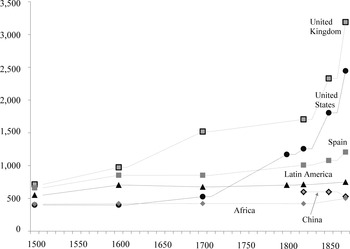
While these arguments are clever and revealing, we find them to be ultimately unsatisfying. Our reservations are both empirical and theoretical. Empirically, the problem is that there are no satisfactory measures of economic performance for North America before the mid-eighteenth century and for Latin America before the late nineteenth century. Except for a few odd national income estimates, measures of GDP are lacking before these dates—a weakness that did not prevent Angus Maddison from concocting numbers to fill the void.Footnote 6 Maddison's original figures, reworked by John H. Coatsworth and depicted here in Figure 1, show North America slightly behind Latin America in the colonial period and both substantially behind the leading countries of Western Europe. Acemoglu, Johnson, and Robinson have put colonial Latin America much further ahead than North America, based on conjectured urbanization rates and a review of Bairoch's very weak estimates of industrial output.Footnote 7 The authors conclude “that the reversal in relative incomes [when the North became richer than the South] took place during the late eighteenth and early nineteenth centuries and was linked to industrialization.”Footnote 8 The truth is that nobody knows when the Great Divergence occurred in the Americas, so explanations of that divergence drift across the centuries without any firm anchor. In this article, we aim to fill the evidential gap using estimates of real wages in leading cities in North and South America between 1500 and 1800.
MADDISON (1995) ESTIMATES OF GDP P.C., IN GEARY-KHAMIS INTERNATIONAL DOLLARS OF 1990

We also find the explanations of divergent development in terms of geography, culture, or institutions to be unsatisfying on the theoretical plane because the discussion is carried on without reference to the markets involved. Most incomes were returns to labor, capital, or land, and reflected the prices of these resources and the quantities owned. The prices are critical, and we focus on the labor market because it determined the incomes of most members of society. Once we see how the markets worked, it is easier to see the role of geography, culture, and institutions in the development of the New World.
The main empirical contribution of this article is the measurement of standards of living in leading parts of North and South America from the early colonial period to the beginning of the nineteenth century. We begin by estimating series of real wages in a group of cities across the continent (Boston, Philadelphia, the Chesapeake Bay, Mexico, Potosi, and Bogota) between colonization and independence, and comparing them to Europe and Asia. We find that for much of the seventeenth and eighteenth centuries, North America was the most prosperous region of the world, offering living standards at least as high as those in the booming parts of North-Western Europe. Latin America, on the other hand, was much poorer and offered a standard of living like that in Spain and less prosperous parts of the world in general. Next, we explore some of the market mechanisms that could have yielded these results including international migration, the demography of the American Indian populations, slavery, and the various labor regimes that the Spanish used to manipulate American Indian labor in the colonial period. We conclude that the long-run income levels in the colonies reflected income levels in the corresponding colonial powers and the Malthusian demography of the Indians. Colonial features like political arrangements, institutions, or culture affected the size of the colony's economy (GDP) but had little bearing on its income level (GDP per capita).
THE PRICE AND WAGE HISTORY OF THE AMERICAS
There have been many studies of both prices and wages for the American continents, but usually they focus on a country or region without a comparative perspective, which is the one we want to stress here. We concentrate on Boston, Philadelphia, and the Chesapeake Bay region of the future United States of America, and Mexico, Potosi, and Bogota in Latin America.Footnote 9 For all of these places, we collected wage rates and the prices of consumer goods. The latter were combined into a consumer price index to gauge the standard of living that workers could purchase with their earnings, calibrating our index so that living standards can be expressed as multiples of the World Bank (Extreme) Poverty Line (WBPL). The following sections discuss the general lines in which we carried out these estimations, and the Appendix available online provides exhaustive details on sources, assumptions, and methods of calculation.Footnote 10
Dealing with Empirical Choices
All studies of this sort confront a series of standard problems regarding the nature of sources, the conversions applied, the type of labor represented, and the kind of wage quotations used. Regarding sources, our data were drawn from price histories conducted by historians of the places that we study. These data were generally derived from the accounts of long-lasting institutions, the records of merchants and manufacturers, the state administrative records, and market reports in newspapers.Footnote 11 Often these sources reported wholesale prices or import valuations rather than retail prices, which are relevant to consumer purchasing power, so in those cases we estimated approximate markups and applied a conversion. Concerning conversions, wages and prices were recorded in units of account like Massachusetts shillings (old tenor and new), Spanish maravedís, and Mexican reales. All units of account have been converted to grams of silver, since silver coins were the principal media of exchange or could be purchased with the paper currencies that sometimes circulated in British North America. Most prices were quoted in local weights and measures, and these have been converted to metric equivalents.
With regards to types of labor, here we concentrate on unskilled workers—generally, building laborers, agricultural laborers, or miners. As is well-known, labor exploitation of various forms was common in the Americas, either as a modified version of precolonial indigenous traditions or as “novel” institutions brought by Europeans.Footnote 12 In all major cities in the continent, unskilled labor markets comprised workers under a variety of contractual arrangements, from extreme forms of coercion to completely free laborers. This study focuses on the section of that continuum where nonvoluntary workers (normally Indians, but sometimes European) met those that were free (mostly European, occasionally Indian or mixed). Slaves are, then, excluded from the present analysis, yet we also include the wages of native Indians employed under labor regimes like repartimiento and mita. While these latter were not voluntary arrangements, earnings can still be meaningfully compared to prices to measure consumption possibilities.Footnote 13 Sometimes wages were paid exclusively in cash, and sometimes they included food, drink, or accommodation. We have focused primarily on cash wages because estimating the value of in-kind payments is difficult. Generally, we have used daily wage rates rather than monthly or annual wages since the latter were much more likely to include unrecorded payments in kind.Footnote 14
Nominal Wages
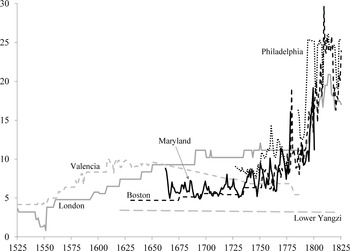
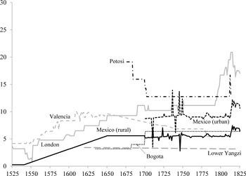
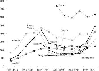
We have been able to assemble unskilled wages for three colonies in British North America—Massachusetts from its founding in 1630, Philadelphia from 1727, and Maryland from 1662.Footnote 15 For Latin America, we have rural and urban wages for Mexico from 1525, Bogota from 1635, and Potosi from 1677.Footnote 16 These have been converted to grams of silver per day based on the silver value of the currency in each year. Figures 2 and 3 summarize our results. For the sake of clarity, we plotted silver wages annually for North America in Figure 2 and for Latin America in Figure 3, in both cases contrasting with silver wages in London, Valencia, and the Lower Yangzi delta, which are meant to illustrate the main patterns in Europe and Asia.Footnote 17 The patterns are striking. Between 1650 and 1700 Potosi had by far the highest wages in the world—almost double those of London, which was in second place. Potosi's lead was not a surprise since it was likely subjected to inflationary pressure as the world's biggest silver mine.Footnote 18 Silver wages elsewhere in the Americas were not exceptional, however. By the early eighteenth century, Potosi's lead had slipped, and between 1750 and 1799 Philadelphia had leapt into first place with the highest wage level in the world. Boston, London, Amsterdam, and Mexico City were close behind. Throughout the early modern period, central and southern Europe had low wage levels as did Bogota and rural Mexico.
NOMINAL WAGES (IN GRAMS OF SILVER PER DAY) IN NORTH AMERICAN CITIES AND AROUND THE WORLD

NOMINAL WAGES (IN GRAMS OF SILVER PER DAY) IN LATIN AMERICAN CITIES AND AROUND THE WORLD

Price of Subsistence
In order to compare living standards across the cities, however, it is necessary to measure the purchasing power of wages over time. High wages in Potosi could have been accompanied by high prices, lowering the purchasing power of wages and eliminating welfare gains. Therefore, wages must be compared to a consumer price index.
Since even the poorest people consume a range of goods, the prices of many things must be taken into account to infer the standard of living from the wage rate. In measuring changes over time, the ideal procedure is to use the results of consumer expenditure surveys to determine the shares of spending on different items and then use those shares as weights in the consumer price index. Our problem is, however, more complicated because we want to measure differences across space as well as changes over time and because diet differed profoundly in different parts of the world. Workers in the Yangtze delta, for instance, subsisted on rice, while their counterparts in Mexico ate maize.
However, despite differences in the staple grain, there were strong similarities in the spending patterns of poor laborers around the world, and these similarities underlie the price indices we construct. Most poor people ate a quasi-vegetarian diet and derived most of their calories from the cheapest available grain. This was either boiled into gruel (e.g., oatmeal or rice) or ground to a coarse flour and fried into unleavened bread (chipatis or tortillas). Peas, beans, or other legumes formed the second important component of the diet and were especially rich sources of protein, although a considerable amount also came from the grain. Some fat (butter, ghee, and olive oil) was also consumed. Meat was rare and consumed mainly on ceremonial occasions. Alcohol was seldom enjoyed. In addition to food, poor laborers also bought some cloth for clothing and used small quantities of fuel for heating or cooking and oil and candles for light. There was also a cost for housing, but it represented only a small fraction of income.
Eighteenth-century descriptions show that the world can be divided into two regions insofar as the consumption of laborers is concerned. Workers in Southern England and the Low Countries were a privileged minority who ate wheat bread, beef, and beer and also had the purchasing power to buy luxuries like sugar, tea, and even pictures for their walls. Elsewhere living standards were much lower.Footnote 19 The quasi-vegetarian diet characteristic of continental Europe was also the norm across Asia. Laboring people across most of Eurasia spent little on items other than food in the eighteenth century, and most of their food spending was directed towards the most economical grain.Footnote 20
Consumption patterns were similar in colonial Latin America.Footnote 21 In Peru, for instance, working-class Indians mostly ate “small girdle cakes of quinoa flour” and roasted maize.Footnote 22 They also consumed small amounts of haricot beans and gourds. Fresh meat was rarely consumed outside of holidays, with some dried meat providing protein in between. Native Peruvians were also limited to crude cooking implements and ovens that filled their homes with soot. These Native Peruvian laborers consumed the same high carbohydrate diet as the poor in other parts of the world.
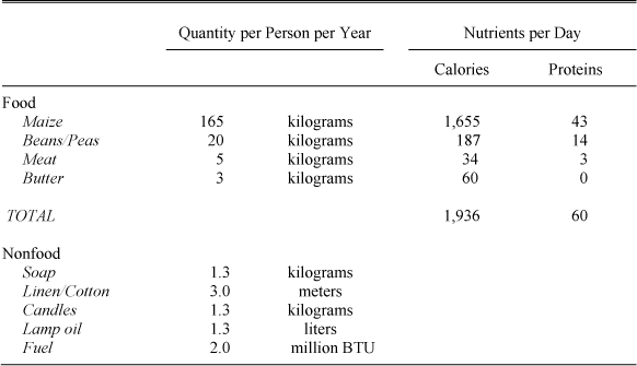
BARE-BONES SUBSISTENCE BASKET OF GOODS
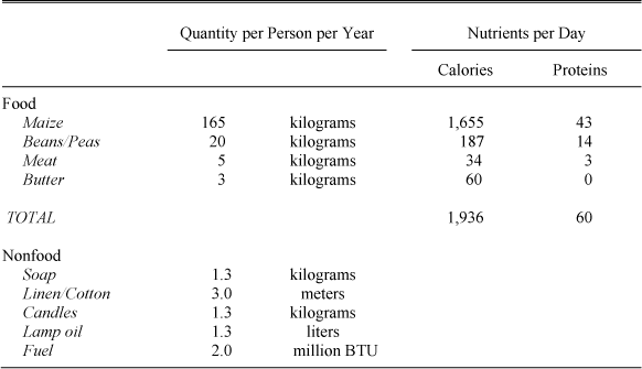
Notes:
The table is based on quantities and nutritional values for the maize diet of the Americas. For other parts of the world, the diet uses the cheapest available grain, and the exact quantities consequently vary. See Allen, “Great Divergence”; and Allen et al., “Wages.”
We use these descriptions to specify a basket of consumer goods representing subsistence consumption for one adult male per year, as shown in Table 1. The total daily intake of calories is set to 1,936—intentionally a modest value. Most calories come from maize and, indeed, it accounts for most of the cost of the basket. We can use this basket for most places in the Americas. For other parts of the world where other grains formed the staple, the diet is modified by replacing the maize with the quantity of oatmeal, millet, sorghum, etc., that brings the total calories in the diet to 1,936. Other items remain the same.
Our cost of living index, therefore, is the cost of purchasing the quantities of each good in the subsistence basket laid out in Table 1.Footnote 23 To compute the index, we gathered prices for the goods in there and converted these prices into silver currency to make them comparable across countries.Footnote 24 The costs of the subsistence baskets are shown in Figure 4.
COST OF SUBSISTENCE (BARE-BONES BASKET, GRAMS OF SILVER PER ADULT MALE PER YEAR) AROUND THE WORLD, 25-YEAR AVERAGES

The cost of living indexes immediately highlight the inflationary effect of the silver economy. Potosi had the highest price level by far, followed by Spain and Mexico. Silver was the most important export of Mexico, so it is not surprising that its prices were elevated like Bolivia's. A considerable proportion of the Potosi and Mexican silver was shipped, in the first instance, to Spain, and its prices were also inflated as a result.Footnote 25 Prices were generally lower in London than in the Spanish Empire, although British prices were also high compared to Central Europe and East Asia, the great sink for the world's silver. Prices were usually lower in British North America than in England. Cheaper commodities were the basis of the staple economies of the east coast of the future United States of America. This pattern was changing at the end of the eighteenth century, as prices in England and the United States of America began to rise with respect to Spain.
Subsistence Ratios
We could measure and compare “real wages” by dividing nominal wages by the price of subsistence, but we can calculate a more revealing real wage index by comparing a laborer's annual income to the cost of supporting his family at subsistence. First, we calculate annual full-time earnings by multiplying the daily wage by the number of days worked in a year. Of course, this varied. The maximum number of working days depended on the number of saint days and religious holidays, but was generally 250–275. For uniformity, we assume 250. Second, we increase the cost of the subsistence basket by 5 percent as an allowance for rent.Footnote 26 Third, we multiply the rent adjusted subsistence basket by 3 to estimate the cost of supporting a family. That cost, of course, varied with family composition, but the assumption that a family's consumption was close to that of three men is justified by the norms for recommended daily calorie consumption. Typically, the calorie consumption of a woman is about four-fifths that of a man, and children receive even less.Footnote 27 Consequently, the recommended calorie intake of one man, one woman, and two children is approximately equal to that of three men.
Thus, the welfare indicator studied in this article—the “subsistence ratio”—equals full-time, full-year earnings of a male unskilled laborer divided by the annual cost of maintaining a family at the subsistence level. If the ratio equaled one, a laborer working full-time earned just enough to keep a family at the subsistence level specified in Table 1. Subsistence ratios greater than one indicate the chance to purchase either more items like those shown in Table 1 or to expand consumption to more “luxurious” items. Ratios less than one suggest that families faced serious economic difficulties. There was little scope for reducing consumption below subsistence, so if the man's income fell short of subsistence either other members of the family had to work more to maintain the minimum standard of living, or some other source of income had to be secured.
The cost of subsistence for a family has another useful interpretation. If we calculate the cost of the subsistence basket in Table 1 (and its counterparts using other carbohydrates) with United States prices in 2005, multiply the result by 3.15 to allow for rent and to convert it to a family basis, and divide by four people per family, the cost per day averages out to be $1.30. This is very close to the World Bank's (extreme) poverty line of $1.25 per day.Footnote 28 Hence, the consumption pattern in Table 1 shows what the World Bank Poverty Line (WBPL) means in practice. A worker with a subsistence ratio of one, by our calculation, earned enough to keep his family at the WBPL. More generally, our subsistence ratio measures the standard of living as multiples of the WBPL.
Previous research has shown two patterns of real wages in early modern Eurasia.Footnote 29 The first pattern characterized the maritime cities of North-Western Europe like London and Amsterdam. They had the highest standard of living. Laborers in these cities earned about four times the WBPL from the fourteenth century to the 1870s when living standards began to rise rapidly. Workers in southern English towns like Oxford had a marginally lower standard of living. This wage pattern is especially surprising considering that North-Western Europe had rapidly rising populations, which could have led to a decline in real wages along Malthusian and Ricardian lines: fertility increases and diminishing returns from a rising land-labor ratio could have overcome any real wage increases. However, the economic growth caused by expanding international trade was enough to offset the rising population and maintain the wage at rough equality.Footnote 30
The second pattern characterized most of continental Europe as well as Asia. In European cities like Vienna and Florence, real wages were almost as high in the fifteenth century as they were in London or Amsterdam. However, the standard of living declined in the next centuries under the impact of growing population and in the absence of a source of growth like the trade boom in North-Western Europe. India suffered a similar drop between the seventeenth and the nineteenth centuries. The standard of living in China was similarly low as well. All of these societies ended up with the wage of unskilled workers equal to 75–150 percent of the WBPL in the late eighteenth century. Surprisingly, Spain followed this second pattern as well. Wages in Valencia and Madrid dropped from four times subsistence in the mid-fifteenth century to only 1.35 WBPL in the eighteenth century. Spain certainly had a colonial empire, but it may have suffered from one that was too valuable. As we have noted, silver was Spain's main colonial import, and the American bullion inflated the Spanish price level. This “Dutch Disease” phenomenon depressed Spanish agriculture and depopulated the medieval industrial centers,Footnote 31 the reverse of the situation in England and the Netherlands where colonies stimulated manufacturing. The population of Spain almost doubled between 1500 and 1800. Without a corresponding increase in the demand for labor, real wages collapsed.
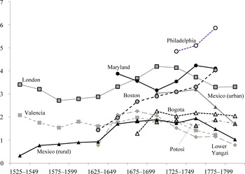
How did the experience of the Americas compare to the European and Asian patterns? Several features stand out from Figure 5, which displays welfare ratios for American, European, and Asian cities from 1500–1800. First, Philadelphia had the highest standard of living for laborers in the eighteenth century, and Boston and the Chesapeake were not far behind. In 1630 living standards for laborers in Boston were below those in London, not dissimilar to those in provincial towns in Southern England, like Oxford.Footnote 32 The standard of living rose in Boston in the seventeenth century, and, by the mid eighteenth, it was above London and almost as high as Philadelphia's. Maryland labor incomes were exceptionally high during the tobacco boom of the 1660s and 1670s and then slid to the London level. North America pulled ahead of London after 1750 as wages advanced slowly in the new world and slumped in the old.
Living standards were much lower in Latin America. Our longest wage series is for Mexico. It begins in 1527 with a wage equal to only one-quarter of subsistence. This was not enough to support a family and barely enough to feed a man for a day. Such low wages undoubtedly worsened the disease mortality that led to a 90 percent drop in the native population in the century and a half following Cortés's conquest. Demography trumped Spanish coercion, however, and decreasing population coincided with increasing wages in rural Mexico, which rose to about 1.75 times subsistence in the late eighteenth century. Wages in other parts of Spanish America were similar.Footnote 33 Laborers in Potosi earned a bit less than twice subsistence in the seventeenth and eighteenth centuries: the very high wages paid in Potosi were indeed cancelled by very high prices. Their counterparts in Bogota earned just over twice subsistence. The highest earning workers in Latin America in our sample were laborers in Mexican cities who earned about three times subsistence in the eighteenth century. This wage, however, was still much less than the wage workers earned in British North America or in North-Western Europe. Using real wages as the metric, the future United States of America was far ahead of Latin America throughout the seventeenth and eighteenth centuries.
WELFARE RATIOS AROUND THE WORLD, 25-YEAR AVERAGES

WAGE PATTERNS AND TRANSATLANTIC INTEGRATED LABOR MARKETS
Why was the unskilled real wage so much higher in North America than in Latin America? We can explain the difference within a simple supply and demand framework. The demand for labor in both continents depended on natural resources, technological efficiency, transportation costs, the ratio of export to import prices, and the quality of political institutions. Improvement in any of these factors raised the demand for labor. However, the long-run supply curve of labor was horizontal in the North and Latin American colonies because international migration and the Malthusian demography of the native population provided a steady supply of labor to the colonies at the respective wage level. The first affected both continents, while the second was important only in Latin America. Therefore, increases in demand would not raise wages but instead increase the population and total GDP of the colony. The wage rate would not be affected and the increase in GDP per capita would be limited to the impact of a greater population on the value of land.
International migration was the major factor determining wages throughout the Americas.Footnote 34 The North American colonies drew labor from Britain so long as they offered a wage that equaled the English wage plus a premium for moving to the New World. Likewise, the Latin American colonies drew labor from the Iberian Peninsula if the same condition was satisfied. Since English wages were twice Iberian wages, the North American colonies faced a higher labor supply curve than the Latin American colonies. Thus, the different wage levels in the colonies originated from the different wage levels in the European countries from which the migrants came.Footnote 35
There are few reliable figures on the actual level of emigration to the Americas, but some estimates suggest that between 1500 and 1800 about 1.5 million Europeans settled in the New World.Footnote 36 These settlers were mostly from Britain or the Iberian Peninsula. In the three periods 1580–1640, 1640–1700, and 1700–1760, there were 293, 248, and 372 thousand immigrants from Britain to its Atlantic colonies respectively. Meanwhile, Spanish immigration was smaller, with 188, 158, and 193 thousand people immigrating in those same three periods. Spanish immigration, however, began earlier with an estimated 140 thousand immigrants traveling to the New World between 1500 and 1580.Footnote 37 Considering that there was also illegal immigration, especially in Spanish America where there were more bureaucratic restrictions to movement, these figures are most likely lower bounds.Footnote 38
Labor market integration was facilitated by a series of institutional arrangements that fostered and regulated European migration to the Americas. More than half of British migrants, for instance, relied on indentured servitude contracts to cover the expensive relocation costs associated with migration.Footnote 39 Given the high productivity of labor in the British Atlantic colonies, most servants successfully completed their contracts and entered a growing free labor market. As the demand for labor increased in the British colonies with the expansion of the staples trade of wheat, tobacco, and rice, more migrants immigrated to the Atlantic colonies. Because immigration was highly sensitive to economic expansion, GDP and population increased at roughly equal rates keeping wage rates or GDP per capita from increasing above the long-run equilibrium level.
Labor markets in Spanish America were more complicated because of the presence of a large native labor market. However, there were still significant flows of immigrants from the Iberian Peninsula to the Spanish colonies. Research on the flow of Spanish migrants has been patchy, making generalizations difficult, but evidence suggests that restrictions to movement imposed by the Crown were often circumvented and people of varied socioeconomic backgrounds were able to migrate to the Americas.Footnote 40 For instance, Castilian immigrants in the colonial period were mostly of middling background, excluding both the extremely rich and the extremely poor. Emigrants maintained contact with their families and often sent for their families after spending some time in the colonies. Thus, there was good information in Spain on the labor market in the colonies, allowing Smithian growth in the colonies to stimulate additional migration from Spain.Footnote 41
However, most laborers in Latin America were natives, and the factors affecting their labor supply in the long run had a profound impact on wages. We hypothesize that the demography of the natives was essentially Malthusian. When wages exceeded subsistence, the population expanded; when wages were lower, it contracted. In the period after 1650, wages were marginally greater than subsistence, inducing a continuous increase in population. From 1650 to 1800, the Mexican population grew from around 1–1.5 million to 6 million. This increase was propelled by a growth in the demand for labor due to technological progress in Mexico. Agriculture was transformed by the integration of European crops and animals (wheat, sheep, and cattle) with the indigenous crops (maize, beans, squash, tomatoes, and chilies). Transportation was revolutionized by European draught animals (horses and mules). Manufacturing gained impetus through the fabrication of new products (woolen cloth) and the concentration of production in specialized regions that promoted the division of labor. The expansion of the Latin American economy took place under the sway of Spanish rule and shows that Spain's policies, however illiberal, were not sufficiently detrimental to prevent economic expansion along Smithian lines.
The expansion was not perfectly smooth and the irregularities provide more support for the Malthusian view. After 1750 there was a slight decline in real wages, consistent with findings of decreasing stature among Mexican army recruits from 1740–1830. Perhaps by the end of the eighteenth century, population growth had outstripped the Smithian expansion leading to a decline in living standards.Footnote 42 In any event, elastic supplies of Indian and Mexican labor stabilized the wage in Mexico at about twice WBPL for a century as the economy developed rapidly and the population expanded.
In conclusion, integrated transatlantic labor markets and the demography of the native population in Spanish America acting together set Spanish American wages at a lower level than wages in British North America. However, this discussion must be tempered with an examination of the forced labor regimes that were so prominent in the Americas during the colonial period.
FORCED LABOR AND WAGES
One of the key features of colonial American economies was the prevalence of coerced labor in its various forms: slavery in North America and the Caribbean and the encomienda, mita, and repartimiento in Latin America. These labor systems, however, were less important in determining wage levels in the colonies than one might expect. White and slave labor were not close substitutes in North America, and forced labor regimes had lost most of their power by the early seventeenth century in Latin America.
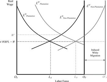
Our analysis does not explicitly include slaves in North America. This could bias our results in two ways. First, because slaves likely had lower earnings than their free counterparts, including slaves in the analysis would decrease the average real wage of laborers in North America.Footnote 43 Factoring in slavery into the average would not affect our figures for Boston or Philadelphia and would not affect our Maryland figures until the eighteenth century when slavery became dominant in the Chesapeake.Footnote 44 However (and secondly), slavery did not have a strong influence on white real wages or discourage white migration to slave holding regions because at least by the eighteenth century, white and black labor were complements rather than substitutes. Throughout the seventeenth century, indentured servants and African slaves provided substitutable labor in the tobacco and rice farms of the Chesapeake Bay region and the Carolinas, but by the eighteenth century, black slaves had replaced indentured servants because they were the cheaper source of labor and additional flows of indentured servants from Britain worked in skilled and management roles.Footnote 45 Indeed, a lower supply price of slaves would have raised white wages in the short run if we assume slaves and free whites were complements, not close substitutes.Footnote 46 This is plausible by the eighteenth century because they performed different functions. Most slaves were employed on plantations producing rice or tobacco. Part of the white economy was also tied to the slave economy through the provision of food and services to the plantations. To analyze the impact of slavery, we conceptually divide the white economy into the part that serviced the plantations and the other part that was independent of plantations. The demand for labor in the two sectors (LDPlantation and LDNon-Plantation) is shown in a standard labor allocation diagram (Figure 6).
SLAVERY AND THE WHITE LABOR MARKET

The demand for white labor related to the slave economy is measured rightwards from the axis at OS and the other demands for white labor are measured leftward from OF. A horizontal line at W = 4 WBPL shows the long-run supply of labor from England. The diagram shows an economy that was, at the outset, in long-run equilibrium with OSLA white labor employed in the plantation-related sector and LAOF elsewhere. Suppose next that the price of slaves in the international market fell. In that case, it would have been profitable for the plantation sector to expand into more remote or less fertile areas, and the demand for white labor in support activities would have risen (to LD’Plantation). The increase in demand would have raised the wage of white workers to W’ in Figure 6 as the plantation sector bid for labor. In the long run, however, the white population of the colony would have grown as migrants arrived in response to the higher wage. This is shown geometrically by the rightward shift in vertical axis on the right side of the diagram. The population would have swollen until the wage in the colony dropped back to W. The increase in the slave economy due to the fall in the price of slaves would have induced an increase in the white population, a short-run rise in its wage, but no permanent improvement in its standard of living, which was set in the British labor market.
The influence of coerced labor in Latin America on real wages was different. We concentrate on the history of Mexico, but the trends in real wages were similar in Bogota and the vicinity (Figure 5), as were the labor market institutions and the reasons for their evolution.Footnote 47 In the 1530s, shortly after Cortés’ conquest, the real wage in Mexico was very low—about 25 percent of subsistence. In the next century, the wage rose gradually towards 2, and it remained at that level in Mexico, Potosi, and Bogota through the eighteenth century.
In the period before 1650, our wages apply to native workers. This was a catastrophic period for the natives whose number fell from about 25 million in 1500 to less than 1.5 million in 1650.Footnote 48 Much of the decline was due to the introduction of Western diseases (small pox, typhus, measles, and influenza), but much was also due to mistreatment and war.
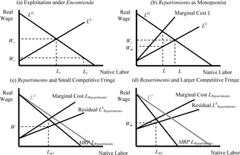
After Cortés's triumph, colonists regarded natives as slaves by right of conquest, and slavery expanded for a few decades after conquest, till the Crown severely curtailed the institution.Footnote 49 An alternative institutional arrangement was regularized through the system of encomienda. Leading conquistadores and political favorites were granted the right to extract labor and tribute from groups of natives. There were few limits on Spanish behavior, and Cortés was not alone in branding and selling his Indians. The major public and private buildings in Mexico at this time were erected by encomienda labor, brutally forced to do the task. Wages were no more than food for the day (perhaps 25 percent of WBPL)—this is shown as We in Panel A in Figure 7—or often zero. Both the quantity and compensation for the labor was dictated by the Spanish, so the natives were driven “off their supply curve.”
Encomienda largely disappeared in the generation after 1550 when it was replaced with less onerous systems of exploitation. Some historians attribute the change to the drop in the native population, but that explanation is hard to credit because labor became more valuable as its supply decreased, enlarging the potential benefits of coercion. A more plausible explanation is that the Spanish Crown preferred wage labor in the colonies and, while consistently opposing the system, allowed the use of encomienda because it was a way of maximizing the rent extracted from Indian labor during the transition to a wage labor market.Footnote 50 As such, encomienda were made non-heritable and regulations were introduced to restrict the rights of encomienda owners. Although some owners finagled a single bequest, eventually they all reverted to the Crown.Footnote 51
ENCOMIENDA, REPARTIMIENTO, AND IMPERFECT LABOR MARKETS

The encomienda was replaced with the repartimiento labor system, which was a compulsory system for obtaining wage laborers. The Crown had hoped that Indian workers could be mobilized by wages, and wages rose in quarter real steps from one-quarter real per day in 1549 to one real per day in 1590 and ultimately 1.75 reales in 1650. Villages were issued quotas of workers to supply at these wages. The village leaders faced sanctions for not complying and could be compelled to participate. This power was limited, however, because Indians drifted away from villages to become casual workers. As population declined in the last half of the sixteenth century, the proportional demands on native villages increased, and villages ceased to supply the laborers demanded irrespective of sanctions. Repartimiento eventually stopped functioning at all and was abolished in 1633, allowing wage labor to become the principal employment system.Footnote 52
Given these historical realities, it is possible to create a model to explain how repartimiento influenced real wages. Because repartimiento was ultimately ineffective in generating a work force, we are inclined to regard Indian labor as essentially voluntary and offered according to a supply curve. The function of the repartimiento was to create an employers’ cartel (a labor monopsony) that could offer lower wages by preventing competition amongst Spanish employers. The equilibrium of the monopsony is shown in Panel B of Figure 7 where the competitive equilibrium (Lc and Wc) is contrasted with the monopsonist's equilibrium (Lm and Wm).Footnote 53 The monoposonist employs Lm workers determined by the intersection of the demand curve and marginal cost of labor from the native economy. The monopsonist pays Wm, which is the wage that induces the supply of Lm. This quantity of labor was shared out amongst the employers who comprised the cartel.
Yet treating the repartimiento as a pure monopsonist overstates its power. The bottom panels in Figure 7 describe a more realistic representation of the Mexican labor market, what is called “a monopsony with a competitive fringe.” In this scenario, there is a dominant firm or cartel, in this case the firms getting repartimiento workers, and a group of outsiders who hire labor in the normal manner. With this arrangement, the labor supply curve shown in the figure should be regarded as the residual supply curve of labor from the competitive fringe, i.e., the total supply to the market less the demand of the fringe for workers.
The dominant employer (the repartimiento) seeks to maximize its profit but has to adjust its wage offer to the competition of other agents in the economy, and that competition limits how much wages can be depressed. In the middle of the sixteenth century, the fringe was small, as described in Panel C. The demand for labor from the repartimiento (its marginal revenue product) made up most of the demand from the whole colonial economy (LD), and the residual supply of labor was not much less than the total labor supply, so the equilibrium (Lm1,Wm1) was probably not far from (Lm,Wm) in Panel B. But the fringe grew substantially as Spaniards acquired native lands for agricultural purposes, making the supply of labor increasingly elastic, as shown in Panel D and reducing the monopsonistic power of repartimiento. By 1620 at least half of the agricultural land in the valley of Mexico had been taken from the Indians and given to colonists mainly in blocks of several hundred acres.Footnote 54 The hacienda was born, and these employers made up much of the fringe.
Two changes governed the evolution of repartimiento: the growth of the hacienda economy in the late sixteenth and early seventeenth centuries increased the demand for labor among the fringe; and the decline in the Indian population reduced the total labor supply. Together they reduced the excess supply of labor in Figure 7. The profit maximizing response of the employer's cartel was to raise the wage in the manner that we have seen occurring. In addition, the growth of the hacienda reduced the share of repartimiento employment, and that directly reduced the power of the employers’ cartel to push the wage below the competitive equilibrium. By the 1620s this power was negligible, repartimiento no longer had a purpose, and it was abolished. Native Mexicans then earned the WBPL.
From then on, the labor market was fundamentally different in two ways. First, labor markets were largely free in the Latin American countries represented in our data set. Although coercive labor such as the mita continued, we are certain that the nominal wages used in Potosi and Bogota reflect the nominal wages of free laborers.Footnote 55 Second, although most laborers continued to be natives, Spaniards began working as laborers, especially in the cities since the wage had risen to Iberian levels. Indeed, international migration set a limit on wages in the Spanish unskilled labor market, just as it had in British North America, although the wage ceiling was lower in Latin America because wages were lower in Spain than in England.
COLONIAL ORIGINS OF THE GREAT DIVERGENCE
The Great Divergence in the Americas was not sparked by the religion or institutions of the conquerors, settler mortality, or geographically determined modes of production but was a product of initial differences in wages between North and Latin America. Over the long run in the colonial period, the growth of per capita income was determined by wages and (we suspect) profit rates in Britain and Spain where the colonies competed for labor and capital, and by the demography of the native population, which expanded in Latin America at similar wage levels to those which induced migration from Spain. Since London offered unskilled workers a wage that was four times the WBPL, while Madrid paid only twice the WBPL, labor incomes in North America were twice those in Latin America for most of the seventeenth and eighteenth centuries. The relative prosperity of North America arose early in the colonial period.
In contrast, the growth of total GDP and population was determined by different factors that were specific to the colonies. These included the efficiency of production, the effectiveness of political institutions, cultural propensities, the healthfulness of the environment, the prices of exported goods, and so forth. Improvements in these regards led to increases in the demand for labor and induced European migration and population growth among the natives. While some historians have argued that North America was advantaged in one or another of these regards, the most striking feature of colonial development is that after the sixteenth century the populations of both North and South America grew rapidly without any prolonged depression of wages. Indeed, they were often rising. It would be hard to argue on the basis of the population histories that bad institutions, bad culture, or bad geography held Latin America back or that North America benefitted from good “fundamentals.” Clearly, various factors influenced the economic expansion of a colony both in total GDP and in population, but because GDP and population were expanding at similar rates, these factors would have little effect on real wages or income per capita.
After independence, these two integrated transatlantic labor markets were broken by the creation of new states with independent immigration and economic policies, yet initial income levels continued to influence later development. Although the post-independence period lies outside the scope of the current article, we speculate that our framework is compatible with two other arguments explaining later divergence between North America and Latin America: Engerman and Sokoloff's emphasis on human capital formation and H. J. Habbakuk's hypothesis that high wages promoted labor augmenting technical change.
Concerning human capital, the widespread commercial activity of the North American staples colonies increased the value of reading and writing for many people, while high wages provided most people with the resources to educate their children—a notable difference from Latin America. In Latin America, lower wages and an agriculture-oriented economy did not provide the same incentives for human capital formation. This is somewhat similar to Engerman and Sokoloff's argument, except we maintain that initial income levels were set by wages in colonial powers rather than by colonial geography and its corresponding mode of production.
In addition, high wages increased the incentive to invent and adopt labor-saving machinery. The invention of labor-saving machinery increased the productivity of labor and wages leading to further invention and wage increases. The result was an ascending spiral of progress in North America but not in Latin America. This conjecture has something in common with Habakkuk's explanation of American industrial preeminence, but there are important differences.Footnote 56 The common feature is the contention that high wages led to labor augmenting technical change; the difference lies in the explanation of the high wages. We attribute them to European wage differences and the demography of Indians in Latin America, while Habakkuk attributed them to free land on the frontier. Since there was lots of “free land” in Latin America as well as in the United States of America, it is hard to see how free land explains North America's development trajectory; indeed, Peter Temin has shown that this link is not consistent with simple general equilibrium models.Footnote 57 Moreover, free land was a colony-specific factor, which, we have argued, affected the size of the new world population, but not the wage.
In conclusion, two streams of migrations in the colonial period—one emanating from North-Western Europe at high wages and the other from Iberia at lower wages—created an early difference in income levels in British and Spanish America. These initial differences were compounded by differences in human capital accumulation and differences in the incentives to mechanize production, which accelerated divergence after independence. Thus, these initial wage differences led to the Great Divergence in the Americas.