1. Introduction

In recent decades, computer simulation has attracted significant interest from philosophers of science. Much of the discussion has centered on how computer simulation compares to other modes of scientific investigation, especially whether it has the same epistemic powers as—and thus might serve as a replacement for—traditional experimentation and observation. This focus is understandable, given that scientists often refer to computer simulation studies as “computer experiments” and sometimes characterize simulation results as “virtual observations.” Nevertheless, a number of important, related questions remain underexplored. For example, it is worth considering not just whether simulation can replace experimentation or observation but also how simulation can work together with these traditional modes of investigation, in order to better achieve scientific aims. This is the topic of the current article, which will offer examples of cooperation between simulation and observation from the fields of meteorology and climate science.

Edwards (Reference Edwards1999, Reference Edwards2010) has made a case already that, in these fields, there is a symbiotic relationship between models and observational data: a mutually beneficial but mutually dependent relationship. However, his focus is primarily on what I will call general model-data symbiosis, in which there are multiple interdependencies among various models and data sets in a field. By contrast, I will be concerned with a more local variety of model-data symbiosis, in which there is two-way interdependence between a particular computer simulation model and data set, or between closely related simulation models and data sets. These local symbiotic relationships are of interest in part because they involve especially close, and two-way, cooperation between simulation and observation. Consequently, however, they also can raise concerns about problematic circularity, for example, if models are tested against data sets that they played some role in constructing.

In section 2, I discuss the idea of model-data symbiosis in more detail and develop the distinction between general and local symbiosis. I then present three examples of local model-data symbiosis in meteorology and climate science, involving data assimilation (sec. 3), targeted observation (sec. 4), and synthetic data (sec. 5). In each case, I show how the local symbiotic relationship works—what the interdependence consists in and how it is supposed to be beneficial—and I consider whether, alongside the benefits, there is any genuine risk of problematic circularity.

2. General and Local Model-Data Symbiosis

Edwards’s (Reference Edwards1999, Reference Edwards2010) notion of model-data symbiosis emerges from his examination of how models and data sets are produced in climate science. On the one hand, complex simulation models of the climate system contain numerous “semi-empirical” parameterizations, that is, observationally derived representations of physical processes that occur on spatial and temporal scales smaller than those that can be explicitly simulated using theory-based equations. This allows for important small-scale processes to be given some representation in these models, rather than none. As a consequence, however, these global climate models are “data laden” (Edwards Reference Edwards1999, 449; Reference Edwards2010, 282). On the other hand, climate data sets are produced with the help of a host of models—not just models of instrument behavior and statistical models used for error detection and interpolation but in some cases computer simulation models too. Some climate data sets, for instance, are a melding of traditional observations and weather forecasts, which help to fill in gaps in the data (see sec. 5). Thus, climate data sets are “model filtered” to various degrees (Edwards Reference Edwards1999, 449; see also Bokulich Reference Bokulich2020). Edwards concludes that, in this domain, models and data have a “mutually constitutive character” (Reference Edwards2010, 433) and enjoy a symbiotic relationship: one that involves mutual dependence but also mutual benefit.

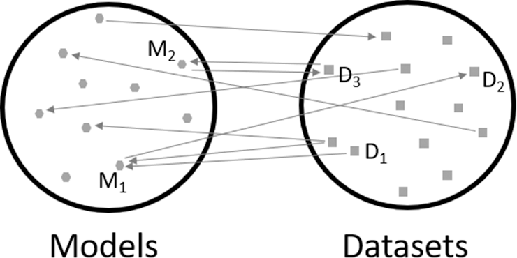
The symbiosis described by Edwards is a feature of a scientific field: in climate science, it is common to have data-laden models and model-filtered data, and these interdependencies are thought to facilitate achieving a number of important aims (e.g., estimating and predicting climate change). Figure 1 depicts this general variety of model-data symbiosis, which holds at the level of a research program or an entire field. Note that, in general model-data symbiosis, there is no requirement that a two-way beneficial relationship holds between any particular model and data set: simulation model M₁ might be constructed with the help of data set D₁, which was not constructed with the help of any simulation model; a different data set D₂, representing a different set of variables or conditions to D₁, might be constructed with the help of that simulation model M₁, and so on.

Figure 1.

General and local model-data symbiosis in a domain of research. Arrows represent beneficial dependencies between individual models and data sets. The many arrows taken together indicate a situation of general model-data symbiosis in the domain of research. A local symbiotic relationship holds between model M₂ and data set D₃.

But we can also envision a more local variety of model-data symbiosis, occurring either within the context of general symbiosis or independently, which involves two-way interdependence between a particular model and data set or between closely related models and data sets. For instance, computer model M₂ might be used in the development of observational data set D₃, which is then used to initialize or evaluate the same, or a closely related, computer model (also depicted in fig. 1). Sections 3–5 will discuss several examples of local model-data symbiosis in the study of weather and climate.

In his discussion of general model-data symbiosis in climate science, Edwards addresses the worry that such symbiosis involves a vicious circularity: “[Symbiosis] is not (or need not be) a form of contamination. Interdependence is not identity; data sets are still derived primarily from observation, and models primarily from theory. Multiple sources of data; multiple, independently developed models; and cross-correlation and intercomparison of all of these make the increasing convergence of climate model results and climate data unlikely to be artefactual” (Reference Edwards2010, 454). Of particular interest has been their convergence on a picture of a warming world: multiple semi-independent simulations that probe the consequences of rising greenhouse gas emissions and other climate-forcing factors (e.g., aerosols, volcanos) increasingly align with multiple semi-independent observationally based estimates of how climate is changing. In other fields, of course, and even with respect to other conclusions within climate science, it may be less clear that model-data convergence is not an artifact of a symbiotic relationship. Moreover, worries about problematic circularity seem especially acute in cases of local model-data symbiosis. In examining examples of local symbiosis below, however, we will see that problematic circularity is only sometimes a genuine concern.

3. Local Symbiosis: Data Assimilation

In numerical weather prediction, a set of dynamical equations that represent physical processes in the atmosphere is used to calculate forecasts of later conditions from a set of initial conditions. The equations are solved at each of many (e.g., thousands or millions of) regularly spaced model grid points, each of which is associated with a volume of atmosphere. The initial conditions for the forecast provide an estimate of the recent state of the atmosphere (its pressure, temperature, winds, etc.) for each of those grid points. How can these initial conditions be obtained? Observations of atmospheric conditions are made every day around the world at ground-based stations, using weather balloons and satellites, via instrumentation on airplanes, and so on, but these observations do not provide uniform, global coverage. To arrive at a complete set of initial conditions, one option is to perform a kind of spatial interpolation among the observations that are available. This was the approach taken in the early days of computer-based weather forecasting.

Today, however, a different approach is used. In data assimilation, observational data and previously generated forecasts (simulation results) are used together to arrive at initial conditions; the simulation results serve as a first-guess estimate of conditions at the time t of interest, providing an estimate for each model variable on the model grid, which is updated in light of observations made around time t (see, e.g., Kalnay Reference Kalnay2003; Parker Reference Parker2017). In this process, the forecast serves as an additional source of information about conditions at t, an estimate generated in light of observations made at an earlier time. Some assimilation algorithms even consider a window of time around t (e.g., a 12-hour window); they attempt to make use of information implicit in the time-ordering of observations when arriving at a best estimate of the atmospheric state for time t. Depending on the details of the algorithm, the state estimate (or “analysis”) of conditions that ultimately is produced can be either a blending of forecasts and observations or a pure model state (i.e., simulation results for time t) selected in light of observations. Such analyses are often characterized as “data products” or as “observationally based” estimates of conditions; in philosophers’ terminology, they are a sophisticated variety of data model.

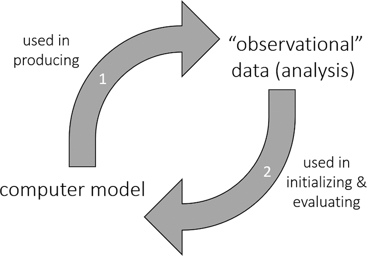
Here, then, weather-forecasting models (computer simulation models) are facilitating the development of analyses (“observational” data sets), which in turn serve as initial conditions for the same (or closely related) weather-forecasting models. In addition, analyses are commonly used to evaluate weather forecasts. To learn about the accuracy of a forecast for time t, the forecast is compared to the analysis for time t—generated with the help of the same (or a similar) forecast model. This is simpler than comparing weather forecasts with observations, because the forecast and analysis are on the same model grid; there is no need to map results from the space of the model (where grid points represent large volumes of atmosphere) to the particular point location where the observation is made (or vice versa), a procedure that itself can introduce error. These symbiotic relationships are represented in figure 2.

Figure 2.

Local model-data symbiosis involving data assimilation.

One might worry, however, that estimates of forecast accuracy obtained by comparing forecasts with analyses will be artificially inflated; perhaps the analyses and the forecasts err in some of the same ways, because of limitations of the computer simulation model involved in generating them both. Indeed, there is some evidence of this: forecasts tend to score best (i.e., are found to have the greatest accuracy or skill) when they are compared with “in-house” analyses, that is, those generated at the same weather-forecasting center, often using the same or a closely related forecast model (see, e.g., Park, Buizza, and Leutbecher Reference Park, Buizza and Leutbecher2008). Here, then, concern about problematic circularity is not entirely unfounded.

But it is important not to exaggerate the problem. For at least some variables, such as temperature, there is quite good agreement among analyses in many regions (Park et al. Reference Park, Buizza and Leutbecher2008). It is also possible to compare forecasts with traditional observations (e.g., of temperature, precipitation, pressure), providing an alternative route to evaluation, at least where observations are available. Moreover, the concern about circularity only arises in connection with forecast evaluation; the use of models to develop analyses for forecast (i.e., model) initialization raises no such concern. In fact, the development and improvement of data assimilation methods for purposes of forecast initialization is seen as one contributor to the significant (and genuine) improvement in forecast skill that has occurred over the last few decades (see, e.g., Kalnay Reference Kalnay2003, 2).

4. Local Symbiosis: Targeted Observation

A second example of local model-data symbiosis can be found in the practice of targeted observation. For high-impact weather events, such as hurricanes, accurate prediction of key characteristics (e.g., hurricane path and intensity) is especially desirable; a poor forecast can result in additional damage to property as well as injury and loss of life to people who are not prepared. Since the behavior of weather-forecasting models is sensitively dependent on initial conditions, one way to reduce forecast uncertainty—at least in principle—is to reduce uncertainty about the initial conditions from which the forecast will be made. The most obvious way to reduce uncertainty about initial conditions is to make additional observations, providing further information to the data assimilation system that generates the analysis/initial conditions.

But making additional observations can be expensive. In the case of hurricanes, for example, additional observations are commonly obtained using specially instrumented aircraft that are flown for the express purpose of making those observations. Given the expense, as well as the limited time available to make observations before the weather event arrives, meteorologists must choose the additional observation sites and variables carefully; they want to make observations that will be especially effective in reducing forecast uncertainty, that is, that will reduce initial condition uncertainty in locations/variables where even small changes mean a relatively large difference in the forecast produced. How can these sensitive locations/variables be identified?

What will not work is simply perturbing the values of variables in the forecast model and seeing how much difference it makes to the forecast that is produced; there are simply too many variables (i.e., millions) and not enough time or computing power. In practice, various methods have been employed, each of which makes use of the forecast model itself or a simplified, linearized version of it (see, e.g., Wu et al. Reference Wu2009). For instance, one approach uses a simplified, linearized version of the forecast model—an “adjoint model”—to trace sensitivities backward in time; the adjoint model allows the calculation of a gradient in a quantity of interest with respect to model input (initial conditions) from a gradient in that quantity with respect to model output (forecasted quantity; see, e.g., Errico Reference Errico1997; Wu et al. Reference Wu, Chen, Lin and Chou2007). In this way, forecasters estimate which locations in the observing region are such that uncertainty about conditions in those locations now is expected to translate into large uncertainty in the forecasted quantity of interest; these sensitive locations can then be targeted for observation.

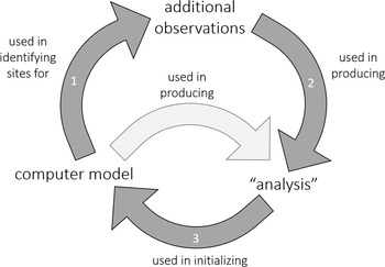
So the local symbiosis in this case works as follows: a forecast model is used to guide the making of additional observations of the atmosphere, in order to produce an improved (reduced uncertainty) estimate of the atmospheric state for a time t, which in turn provides initial conditions for the forecast model, whose forecasts now hopefully are less uncertain in precisely those respects that are of particular interest (e.g., the pathway of a hurricane). Indeed, the forecast model might be used not just in guiding the selection of observing sites/variables but also in performing the subsequent data assimilation that generates the state estimate for t. Figure 3 depicts this local symbiosis.

Figure 3.

Local model-data symbiosis involving targeted observation. The lighter arrow represents the use of the forecast model in data assimilation (see sec. 3).

Focusing on the primary symbiotic relationship under discussion (represented by the darker arrows in fig. 3), there does not seem to be much threat of problematic circularity. The value of targeted observations can be investigated by comparing the accuracy of forecasts with and without the extra observations collected and, even if forecast accuracy is calculated relative to analyses, there is no reason to think that the evaluation would artificially favor one set of forecasts (e.g., those with the extra observations) over the other. Because the production of the analysis involves data assimilation (represented by the lighter arrow in fig. 3), however, the possibility of problematic circularity noted in the previous section is present.

In practice, studies so far have tended to find only a mixed/small forecast advantage from targeted observations (Majumdar Reference Majumdar2016). There are a number of possible reasons for this. Most obviously, it could stem from limitations of the forecast models themselves, for example, distortions in how they represent key atmospheric processes. In addition, methods like adjoint modeling are efficient because they involve a linear approximation to a nonlinear process, that is, the unfolding of atmospheric conditions; in weather situations involving strong nonlinearity, these methods can give less accurate results, even when forecast models are of high quality. Given the significant costs involved, the operational use of targeted observation remains relatively limited at present; it is of greatest interest in situations of very-high-impact weather.

5. Local Symbiosis: Synthetic Data for Benchmarking

Time series of temperature and other variables collected at land-based weather observing stations are a valuable resource for climate scientists investigating long-term climate change. These time series in some cases extend back a century or more, whereas other sources of data (e.g., satellites) cover only more recent periods. But these time series also can contain spurious jumps and trends, stemming from various factors: an instrument is moved from one side of a building to another at an observing site, a new instrument replaces an old one, a new observing technique or time is adopted, and so on. Station metadata reporting such changes in instrument siting and observing practices are very useful when it comes to identifying spurious jumps and trends, but such metadata are often absent. In practice, statistical “homogenization” algorithms are applied to try to identify and remove such artifacts (or “inhomogeneities”), so that changes found in observational data reflect real changes in climate (see, e.g., Costa and Soares Reference Costa and Soares2009; Cowtan Reference Cowtan2015). Such an algorithm, for example, might seek to identify artifacts by looking for a change in the way that temperature observations made at an observing station tend to deviate from those made at nearby observing stations.

How can such homogenization algorithms be evaluated? After all, climate scientists cannot go back in time and measure again; they do not have access to the “true” past temperature values. One approach is to test homogenization algorithms on “synthetic data”—time series generated to contain artifacts similar to those that plausibly are present in the real data.Footnote ¹ Synthetic data can be generated via statistical methods: time series are produced that display certain statistical properties (e.g., related to variation and autocorrelation) similar to those expected in homogeneous data, and then artifacts/inhomogeneities like those thought to be present in real data are added (see, e.g., Venema et al. Reference Venema2012). Another approach, currently envisioned in connection with the development of a publicly available database of surface temperature observations, will use climate model simulations as the “true” or “clean” data to which artifacts are added (Rennie et al. Reference Rennie2014). Unlike statistically produced time series for small networks of stations, the simulation-generated data will have global coverage and consequently will include more physically coherent spatiotemporal variability (e.g., associated with events like El Niño–Southern Oscillation; Willett et al. Reference Willett2014). Whatever method is used to generate the artifact-containing synthetic data, the question is to what extent a homogenization algorithm successfully recovers the “clean” data. For the best test, of course, algorithm developers should not be told too much about the artifacts that will be present.

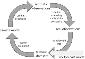
A local symbiotic relationship emerges once we consider subsequent uses of homogenized data. Either on their own or in conjunction with other information, these data are a key ingredient of climate data sets, including so-called reanalysis data sets. Reanalysis data sets are produced by dividing a past period (e.g., of several decades) into consecutive short time windows (e.g., 12 hours) and performing data assimilation for each of those windows, generating a long sequence of analyses.Footnote ² Climate data sets, including reanalysis data sets, are used for many purposes in climate research—not just for estimating how much climate has changed but also for evaluating climate models. Thus, we can have climate models facilitating the production of synthetic data, which are used to evaluate homogenization algorithms for processing real data, which are transformed (via homogenization and perhaps data assimilation) into climate data sets, which are used in evaluating climate models—including perhaps the very climate models originally used in generating the synthetic data. This complex, local symbiosis is depicted in figure 4.

Figure 4.

Local symbiosis involving synthetic data. The lighter arrow represents the optional use of data assimilation.

This sort of symbiosis carries a relatively low risk of problematic circularity. Suppose a homogenization algorithm is chosen because it did a good job of removing known artifacts from synthetic data generated with the help of a particular climate model, C. There is little reason to think that a climate data set obtained by applying that homogenization algorithm to real data would fit better with simulations from C than with simulations from other climate models. After all, C has no direct role in producing the climate data set; it merely plays a supporting role in efforts to evaluate methods for removing artifacts when producing the data set. The most plausible threat of problematic circularity once again seems to be that due to the use of data assimilation, which is employed in producing only some climate data sets (i.e., reanalysis data sets). In particular, since weather-forecasting models (used in data assimilation) and climate models take a similar approach to representing physical processes in the atmosphere, it could be that reanalysis data sets and climate simulations have some shared errors. However, when variations in temperature and precipitation in fields from climate models and reanalysis data sets are examined, it turns out that reanalysis data sets appear to be more similar to one another than to climate simulations (Masson and Knutti Reference Masson and Knutti2011), which goes some way toward alleviating this worry.

6. Conclusion

The foregoing discussion has called attention to local, model-data symbiosis in the fields of meteorology and climate science. In contrast to the general model-data symbiosis identified by Edwards (Reference Edwards1999, Reference Edwards2010), which involves multiple interdependencies among various models and data sets in a field, local model-data symbiosis involves two-way interdependence between a particular simulation model and data set or between closely related models and data sets. In each of the examples of local symbiosis presented above, a simulation model aids in the production of one or more data sets, which in turn is used to initialize or evaluate that same (or a related) simulation model.

As those examples illustrated, such interdependence can, but need not, involve some problematic circularity. If simulation results directly shape the content of a data set, and the data set is then used to evaluate the simulation model that produced the results (or even the very same simulation results), then the apparent skill or accuracy of the model can be artificially inflated. But if those data sets are used only to initialize the simulation model—not to evaluate it—or if simulation results only play an indirect role in the development of a data set (e.g., as a test bed for evaluating data-processing methods, rather than directly shaping the content of the data set) that is subsequently used to evaluate the simulation model, then there is little, if any, risk of such circularity.

While the issue of circularity merits consideration, it is important not to lose sight of the benefits that local model-data symbiosis can bring. In the examples discussed here, from meteorology and climate science, these benefits include arriving at initial conditions that result in better weather forecasts, evaluating weather forecasts and climate simulations in a more straightforward and convenient way, gaining insight into the kinds of artifacts that may go undetected in climate data sets, and more. Analyzing examples of local model-data symbiosis in other fields (e.g., Bokulich Reference Bokulich2018) may shed further light on the valuable ways in which computer simulation can cooperate with traditional modes of scientific investigation like experimentation and observation, regardless of whether it can replace them.