

Introduction
China has achieved impressive economic growth during the last three decades due to rapid industrialization that has been facilitated by the creation of Special Economic Zones. In addition, the internal migration of over 150 million workers from rural to urban areas (Hu et al., Reference Hu, Cook and Salazer2008; Chan, Reference Chan2013) has been critical for economic development. However, migration has separated married couples for extended periods and has potentially lowered measures of self-reported health (Chen et al., Reference Chen, Liu, Vikram and Guo2015). China’s crude divorce rate, measured by number of divorces per 1000 population, increased from 0.33 in 1979 to 2.8 in 2015 (Ministry of Civil Affairs of the People’s Republic of China, 2015). Moreover, enforcement of the one-child policy since 1979 has intensified the patrilineal emphasis on sons (Sun & Zhao, Reference Sun and Zhao2014) and can differentially affect men’s and women’s chances of divorce. While the effects of rapid industrialization on air pollution are evident in Chronic Obstructive Pulmonary Disease prevalence (Gao & Prasad, Reference Gao and Prasad2013), the effects on family structures, marital dissolution and individual well-being are complex (e.g. Mascie-Taylor & Krzyzanowska, Reference Mascie-Taylor and Krzyzanowska2017). It is important to conduct comprehensive analyses of data from China to understand the inter-relationships between internal migration, marital dissolution and well-being.
Modelling the inter-relationships between migration, divorce and well-being requires a long time frame since the effects of explanatory variables on outcomes are likely to be gradual and there is heterogeneity in couples’ circumstances. The availability of nine waves of data from the China Health and Nutrition Surveys (CHNS) during 1989–2011 provides a unique opportunity to investigate at least three sets of hypotheses that are useful for the specification of empirical models. First, the frequency and durations of husbands’ and wives’ migration are likely to differentially affect their chances of divorce and indicators of health and well-being. For example, men and women from rural areas working in urban settings are exposed to modern aspects of social life that can increase the chances of divorce. Moreover, living conditions for poor migrants may not be conducive to healthy lifestyles such as the availability of nutritious meals at affordable prices; extended separation periods can lower the health status of migrants.
The study’s second hypothesis is that, due to patrilineal family structures, husbands in unhappy marriages with a first-born daughter might be inclined to divorce and re-marry with the expectation of producing a son; such pressures need not apply to wives. This is especially relevant for China due to the one-child policy. Thus, the gender composition of surviving children (Muhuri & Preston, Reference Muhuri and Preston1991; Bhargava, Reference Bhargava2003a) is likely to have differential effects for husbands’ and wives’ chances of marital dissolution. While the inter-dependence of family members’ decisions is recognized in social sciences (Mincer, Reference Mincer1962; Bhargava, Reference Bhargava1997), it is important to investigate asymmetries in the divorce decisions of Chinese couples (Xu et al., Reference Xu, Yu and Qiu2015). Estimation of comprehensive probit models for the chances of divorce controlling for unobserved heterogeneity can shed light on these issues.
It is important to augment the analyses of self-reported measures of health with objective physiological measures such as blood pressures, which are affected by domestic tension. Accordingly, the third hypothesis is that couples in unhappy marriages could experience elevated blood pressure levels that might be reduced by amicable separation so that divorce might have beneficial effects for health (cf. Waite & Gallagher, Reference Waite and Gallagher2000). By contrast, the self-reported health of husbands and wives is a subjective assessment that can be influenced by increased earnings due to migration. Longitudinal data on self-reported health and systolic and diastolic blood pressures are available in four waves of the CHNS during 1997–2006 and can facilitate dynamic modelling of the factors affecting health and well-being. This is important for China where divorce rates are still relatively low and social and economic pressures against marital dissolution can complicate the interpretation of findings.
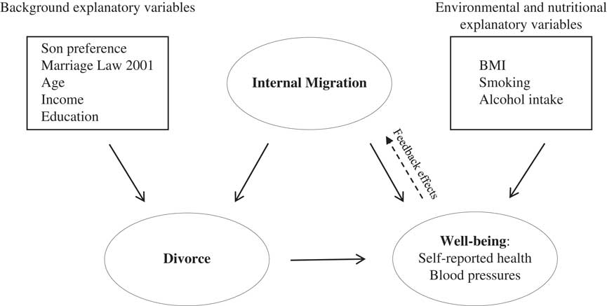
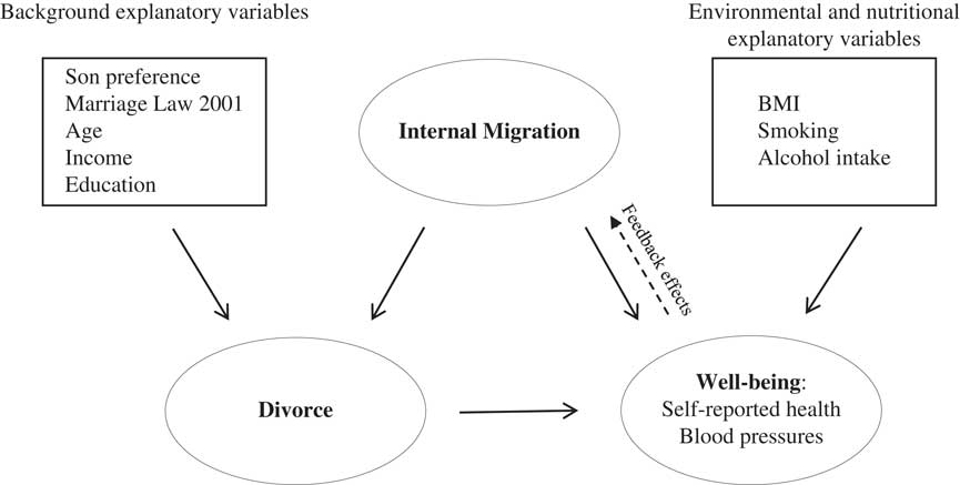
Several methodological issues need to be tackled to draw robust inferences from empirical models. For example, while it is important to explain individuals’ chances of migration by measures reflecting health status, previous researchers have primarily estimated cross-sectional models (e.g. Tong & Piotrowski, Reference Tong and Piotrowski2012). Such models cannot account for the dynamics in the inter-dependence between outcomes. Moreover, couples’ health is likely to be influenced by the frequency and durations of migration spells, which can introduce feedback effects (‘simultaneity’) into the relationships. It is useful to employ econometric methods for longitudinal data (Bhargava & Sargan, Reference Bhargava and Sargan1983) to investigate inter-relationships. The estimation of dynamic random effects models for self-reported health and blood pressures, incorporating the additional aspects discussed below, can provide insights into the effects of divorce on health in China. Figure 1 shows the salient aspects of these inter-relationships.
Graphical representation of the empirical models for the inter-relationships between internal migration, divorce and well-being in China.
Methods
Data
The China Health and Nutrition Surveys (CHNS) were conducted by the Carolina Population Center, Institute for Nutrition and Food Hygiene, and the Chinese Academy of Preventive Medicine (Du et al., Reference Du, Lu, Zhai and Popkin2002). A multistage clustering design was used to draw the sample in nine Chinese provinces (Liaoning, Heilongjian, Shandong, Jiangsu, Henan, Hubei, Hunan, Guangxi and Guizhou). The counties in the provinces were stratified by income (low, middle and high) and a weighted sampling scheme was used to randomly select four counties in each province. Villages and townships within counties and neighbourhoods in cities were randomly selected. The longitudinal cohort consisted of 7132 households with over 19,000 individuals observed in nine survey waves during 1989–2011. Previous analyses of the data indicate that CHNS households were comparable to national samples (Short et al., Reference Short, Ma and Yu2000; Entwisle & Chen, Reference Entwisle and Chen2002).
The CHNS compiled demographic variables such as gender, ethnicity, age, household’s location in rural and urban areas and household size. Adult members’ marital status and the numbers of male and female children were recorded. Education levels were recorded and a categorical variable was created that ranged from 0–6, with ‘6’ reflecting a postgraduate degree. The per capita and total household incomes were constructed from the responses to various items.
Internal migration patterns were investigated for individuals by inquiring whether they had been away from home and the duration in months. The questions were typically answered by the head of the household though other members were approached if the household head was unavailable. Note that in view of the practice of parents living with adult children in China, in households comprising a married couple and children the ‘respondent’ and ‘spouse’ would be the husband and wife. There were changes in the questionnaires from 1997 pertaining to months that individuals were away; numbers of months away were inquired for all household members whenever possible during the survey rounds. The numbers of months that husbands and wives were away were used to create time-varying variables for migration durations in 1989–2011 in the ‘unbalanced’ panels that were used to model the chances of marital dissolution. In the analyses of self-reported health and blood pressures, numbers of months that husbands and wives were away at four time points in 1997–2006 were averaged to reduce missing observations in the ‘balanced’ panels. Lastly, indices of internal migration were created by summing the binary responses to whether husbands and wives had been away during each of the nine survey rounds.
The self-reported health of individuals was inquired in four survey rounds in 1997–2006 on a scale 1–4, which was transformed so that 1 and 4 indicated, respectively, ‘poor’ and ‘excellent’ health status. Moreover, individuals’ systolic and diastolic blood pressures were measured in all survey rounds using a spirometer. The heights of individuals were measured using Shorr boards; weight was measured in all survey rounds using electronic scales that had been calibrated. The questionnaires inquired if individuals were smokers and recorded the number of cigarettes smoked daily. Alcohol consumption was inquired and an index was constructed by summing the amount of beer, wine and liquor consumed per week.
Analytical framework and empirical models
The problems of internal migration and individual health are dynamic in nature in China due to rapid industrialization; the availability of jobs in the Special Economic Zones has fuelled the flow of millions of workers from rural areas. Moreover, the extent to which migrants can work under difficult conditions depends on their health status (e.g. Mou et al., Reference Mou, Cheng, Zhang, Jiang, Lin and Griffiths2009); the problems are compounded by inadequate facilities for migrants with their hukou (household registration) in rural areas. Previous research on China has not simultaneously addressed such issues. While Tong and Piotrowski (Reference Tong and Piotrowski2012) explained the chances of internal migration by self-reported health using CHNS data, Chen et al. (Reference Chen, Liu, Vikram and Guo2015) explained self-reported health by dichotomous variables for the spouse being away. The analytical framework for modelling the inter-relationships between internal migration, marital dissolution and well-being incorporated the three hypotheses outlined in the Introduction and certain related aspects.
First, migration to urban areas in China has afforded employment opportunities for the rural poor and has reduced poverty levels via remittances (money sent home by migrant workers) (World Bank, 2011). From the standpoint of specification of empirical models for outcomes such as marital dissolution and health status, internal migration is an important explanatory variable. The first set of models investigated the effects of husbands’ and wives’ migration frequencies and durations for the chances of marital dissolution. Because time spent away from home can be stressful for marital relationships, it is important to employ flexible models to investigate if husbands’ and wives’ migration durations affected their chances of divorce.
Second, it has been argued that marriage has benefits for individuals’ health and happiness in countries such as the US and that divorce often has adverse consequences (Waite & Gallagher, Reference Waite and Gallagher2000). However, such analytical frameworks need not extend to China, where divorce rates were below 5% even in 2011. This is because unhappy couples may not divorce due to social pressures unless the relationship is unbearable. The Marriage Law amendment of 2001 in China extended greater inheritance and maintenance rights to women and has facilitated marital dissolution. Thus, it is important to investigate the effects of divorce on indicators such as self-reported health using dynamic models that allow previous health status to affect current health. An indicator variable can be included for individuals who divorced during the sample period to investigate if divorce had negative effects on health status.
Third, models for systolic and diastolic blood pressure levels of husbands and wives can provide substantive insights into the effects of divorce on health. Moreover, it is plausible that individuals’ migration durations are correlated with the errors affecting the models for blood pressures. For example, individuals in poor health may not be able to work away from home for extended periods so that the errors affecting the model for blood pressures might be correlated with migration durations. Such issues can be tackled using econometric methods for longitudinal data. Moreover, China is experiencing increases in obesity due to dietary and lifestyle changes (Whang et al., Reference Whang, Zhai, Zhang and Popkin2012), and this needs to be taken into account in the empirical models.
The preceding discussion enables the specification of models for individuals’ chances of divorce, and for self-reported health and systolic and diastolic blood pressures. The random effects probit model for chances of divorce of the i th husband (wife) in time period t can be written as:
 $$\eqalignno{ & \left( {{\rm Divorce}} \right)_{{it}} \,a_{0} {\plus}a_{{\rm 1}} \left( {{\rm Indicator}\,{\rm rural}\,{\rm areas}} \right)_{i} {\plus}{a}_{{\rm 2}} \,{\rm ln}\left( {{\rm Age}} \right)_{{it}} {\plus}a_{{\rm 3}} \left[ {{\rm ln}\left( {{\rm Age}} \right)_{{it}} } \right]^{{\rm 2}} \cr & \qquad {\plus}a_{{\rm 4}} \,{\rm ln}\left( {{\rm Age}\,{\rm difference}} \right)_{i} {\plus}a_{{\rm 5}} \left( {{\rm Education}} \right)_{i} \cr & \qquad {\plus} a_{{\rm 6}} \,{\rm ln}\left( {Per\,capita\,{\rm household}\,{\rm income}} \right)_{{it}} {\plus}a_{{\rm 7}} \,{\rm ln}\left( {{\rm Months}\,{\rm away}-{\rm husband}} \right)_{{it}} \cr & \qquad {\plus}a_{{\rm 8}} \,{\rm ln}\left( {{\rm Months}\,{\rm away}-{\rm wife}} \right)_{{it}} {\plus}a_{{\rm 9}} \left( {{\rm Number}\,{\rm of}\,{\rm sons}} \right)_{{it}} {\plus}a_{{{\rm 1}0}} \left( {{\rm Marriage}\,{\rm Law}\,{\rm 2}00{\rm 1}} \right)_{{it}} \cr & \qquad {\plus}u_{{it}} \left( {i\, {\equals}\, {\rm 1},...,N;\,t\, {\equals}\, {\rm 1},\,\ldots\,,J_{i} } \right) $$
Here ‘ln’ represents natural logarithms; ‘Age difference’ is the difference between couples’ ages and ‘Months away’ is the time spent working away from home. Both husbands’ and wives’ time away from home in months were included in the model; these variables were replaced by the migration index, which summed the binary responses for whether the individual had been away. However, coefficients of the time the spouse spent away from home were not significantly different from zero and these variables were dropped to enhance the efficiency of the parameter estimates. Also, individuals were dropped from the sample in subsequent periods if they had divorced.
The model in equation (1) was an ‘unbalanced panel’ in that different numbers (J i ) of time observations were available for the i th individual. The model was initially estimated by pooling the data for husbands and wives and by including an indicator variable for wives. Likelihood ratio tests rejected the null hypothesis that the model parameters were constant across the two groups and the results are reported separately for husbands and wives. Note that eight indicator variables were included in the model in equation (1) to account for differences in means of variables in the provinces; eight indicator variables were included to account for differences in means over time. The u it values were error terms that can be decomposed in a simple random effects fashion as:
 $$u_{{it}} \, {\equals}\, \delta _{i} {\plus}v_{{it}} $$
where δ i were individual specific effects that were assumed to be normally distributed with zero means and constant variance; v it values were normally distributed variables with zero means and constant variance.
The dynamic random effects model for self-reported health is not spelled out to economize on space; it was similar to the model for systolic (and diastolic) blood pressure for husbands (wives):
 $$\eqalignno{ & {\rm ln}\left( {{\rm Systolic}\,{\rm BP}} \right)_{{it}} \, {\equals}\, b_{0} {\plus}b_{{\rm 1}} \,{\rm ln}\left( {{\rm Age}} \right)_{{it}} {\plus}b_{{\rm 2}} \left[ {{\rm ln}\,\left( {{\rm Age}} \right)_{{it}} } \right]^{{\rm 2}} {\plus}b_{{\rm 3}} \left( {{\rm Education}} \right)_{i} \cr & \qquad {\plus}b_{{\rm 4}} \,{\rm ln}\left( {{\rm Months}\,{\rm away}\!-\!{\rm husband}} \right)_{i} \cr & \qquad {\plus}b_{{\rm 5}} \left[ {{\rm ln}\left( {{\rm Months}\,{\rm away\!-\!\rm husband}} \right)_{i} } \right]^{{\rm 2}} {\plus}b_{{\rm 6}} \,{\rm ln}\left( {{\rm Months}\,{\rm away}\!-\!\ \!\!\rm wife}} \right)_{i} \cr & \qquad {\plus}b_{{\rm 7}} \left[ {{\rm ln}\left( {{\rm Months}\,{\rm away\!-\!\rm wife}} \right)_{i} } \right]^{{\rm 2}} {\plus}b_{{\rm 8}} \left( {{\rm Divorce}} \right)_{{it}} {\plus}b_{{{\rm 11}}} \,{\rm ln}({\rm BMI})_{{it}} \cr & \qquad {\plus}b_{{{\rm 12}}} \,{\rm ln}\left( {{\rm Systolic}\,{\rm BP}} \right)_{{it{\minus}{\rm 1}}} {\plus}u_{{{\rm 2}it}} \left( {i\, {\equals}\, {\rm 1},...,N;\,t\, {\equals}\, {\rm 2},{\rm 3},{\rm 4}} \right) $$
Note that the dynamic models for individuals’ self-reported health and systolic and diastolic blood pressures were estimated using four time observations during 1997–2006. Because the estimation methods required ‘balanced panels’, there was a reduction in the sample sizes that was likely to affect mainly the coefficients of constant terms (Wang et al., Reference Wang, Wang and Carroll1997). The previous levels of blood pressure were postulated to affect current levels (Bhargava, Reference Bhargava2003b) thereby enabling a distinction between the short- and long-run effects of explanatory variables. For example, short-run ‘elasticity’ of systolic blood pressure with respect to BMI (weight in kilograms divided by squared height in metres; Cole, Reference Cole1991) was b 11; the long-run elasticity was b 11/(1−b 12). Note that household income was not a significant predictor in the models for blood pressures and was excluded from this model.
Statistical and econometric methods
The probit model in equation (1) for individuals’ chances of divorce was estimated by maximum likelihood using an algorithm in Stata Version 14 (Stata, College Station, TX). Maximized values of the log-likelihood function were used to test the constancy of model parameters for husbands and wives. Multiple imputations (Rubin, Reference Rubin1987) were used to assess the effects of missing observations on the estimated coefficients.
The dynamic random effects models for self-reported health and systolic and diastolic blood pressures were estimated by maximum likelihood. Self-reported health was treated as a continuous variable partly because the model was dynamic and also because the errors were likely to be serially correlated; ordinal regression models (McCullagh, Reference McCullagh1980) were also estimated using cross-sectional data. The distribution theory assumed that the number of individuals (N) was large but that the number of time periods (T) was small. Previous observations on dependent variables such as blood pressure were treated as correlated with the errors (‘endogenous’) (Anderson & Hsiao, Reference Anderson and Hsiao1981; Bhargava & Sargan, Reference Bhargava and Sargan1983). Realizations of certain time-varying explanatory variables in different survey rounds were assumed to be uncorrelated with the errors (‘exogenous’). The errors (u 2it ) were assumed to be independent across individuals but correlated over time with a positive definite variance–covariance matrix; the random effects decomposition in equation (2) was a special case and the null hypothesis was tested using likelihood ratio tests. A numerical optimization routine (E04 JBF) (Numerical Algorithm Group, 1990) was used in a FORTRAN program to compute maximum likelihood estimates. Asymptotic standard errors of the parameters were computed by numerically approximating second derivatives of the maximized log-likelihood functions.
Further, certain explanatory variables in the model in equation (3) might be correlated with the random effects (δ i ). Maximum likelihood methods can be used for consistent and efficient estimation of the model parameters and to test the ‘exogeneity’ null hypothesis. Assuming that n 1 and n 2 time-varying variables x 1 and x 2 were exogenous and endogenous, respectively, the correlation between the errors and x 2 values was tackled by postulating the pattern:
 $$x_{{2ijt}} \, {\equals}\, \lambda _{j} \,\delta _{i} {\plus}x^{{\asterisk}} _{{2ijt}} $$
where
 $x^{{\asterisk}} _{{2ijt}} $
was uncorrelated with δ
i
. This correlation pattern has the advantage that deviations of x
2ijt
values from their time means can be used as additional (T−1) n
2 ‘instrumental variables’ to facilitate estimation of the parameters. The null hypothesis of zero correlation between the random effects and migration durations was tested in the models for blood pressures. Given four time observations, the likelihood ratio statistic was distributed for large N values as a chi-squared variable with four degrees of freedom.
Results
Descriptive statistics for husbands and wives
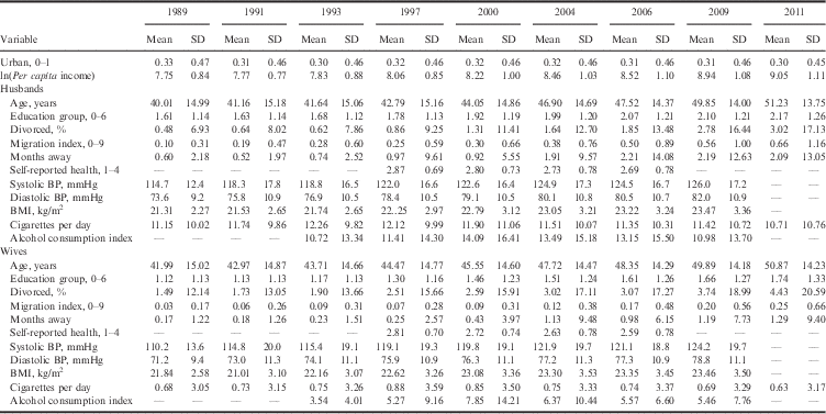
Table 1 reports the descriptive statistics for the salient variables in nine survey rounds of the CHNS; the results are presented separately for husbands and wives for comparisons. Approximately 32% of respondent households were in urban areas. At the start of the surveys in 1989, the mean annual per capita household income in 2011 prices was 3072 yuan. There was a steady increase in household incomes and mean per capita income in 2011 was 13,480 yuan, showing a 4-fold increase.
Sample means and standard deviations of variables for husbands and wives in the China Health and Nutrition Surveys, 1989–2011Footnote a

a In the unbalanced panel, data on 4324 husbands and wives were used on average in the nine survey rounds to compute the sample means.
The mean ages of husbands and wives in the household in 1989 were 40.01 and 42.0 years, respectively. The mean educational attainment for husbands in 1989 was 1.61, which was significantly higher (p<0.05) than the mean of 1.12 for wives. While the mean percentages of divorced men in the survey households increased from 0.48% to 3.02% from 1989 to 2011, the corresponding figures for women were 1.49% and 4.43%, respectively. The means of the migration index based on binary responses in 1989 and 2011 for husbands were 0.10 and 0.66, respectively. The corresponding means for wives were 0.03 and 0.25, respectively, showing that men had been away from home more frequently. Similarly, the mean numbers of months for which husbands were away from home in 1989 and 2011 were 0.60 and 2.09, respectively; the corresponding means for wives were 0.17 and 1.29, respectively. Bivariate correlations between the migration index and numbers of months that husbands and wives were away were between 0.50 and 0.60.
The mean levels of self-reported health for husbands for the ‘balanced panel’ in 1997, 2000, 2004 and 2006 were 2.87, 2.80, 2.73 and 2.69, respectively. There was a decline with age in the self-reported health of husbands and also for wives. The mean systolic and diastolic blood pressures were significantly higher for husbands in all survey rounds. By contrast, means of the BMI were similar for husbands and wives and the differences were generally not significant. There were significant differences in the smoking and alcohol consumption patterns of husbands and wives. For example, the mean numbers of cigarettes smoked daily by husbands in 1997, 2000, 2004 and 2006 were 12.12, 11.90, 11.51 and 11.35, respectively. The corresponding figures for wives were 0.88, 0.85, 0.75 and 0.74, respectively. The index of alcohol consumption was significantly higher for husbands in all survey rounds.
Husbands’ and wives’ chances of divorce
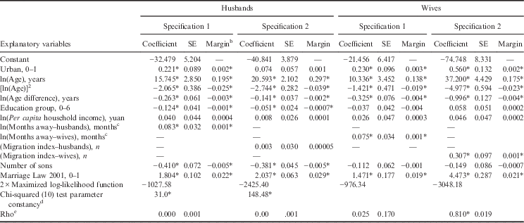
Table 2 presents the results from estimating the random effects probit models for husbands’ and wives’ chances of divorce using nine waves of CHNS data. Initially, the data were pooled for husbands and wives and the model parameters were estimated by maximum likelihood. However, likelihood ratio statistics for Specifications 1 and 2 in Table 2 were 31.0 and 148.48, respectively, rejecting the null hypotheses of parameter constancy for the two groups. Note that Specification 1 used the numbers of months that husbands and wives were away from home, whereas Specification 2 replaced this variable by the migration index based on number of times they reported being away. The ‘marginal effects’ of explanatory variables were computed at the sample means and are reported in Table 2.
Maximum likelihood estimates of random effects probit models for the chances of divorce for husbands and wives using data from nine waves of the China Health and Nutrition Surveys, 1989–2011Footnote a

a Values are maximum likelihood estimates of the coefficients and their standard errors from ‘unbalanced panels’ using data on 4324 husbands and wives.
b Marginal effects were computed at the sample means.
c Numbers of months away for husbands and wives were used in the respective models for husbands and wives; similarly for the migration index.
d Chi-squared statistics for testing if the model parameters were the same for husbands and wives.
e Rho is proportion of the variance contributed by random effects.
*p<0.05.
The main finding in Table 2 is that the chances of divorce for husbands and wives in urban areas were significantly higher than in rural areas (p<0.05). Also, there were non-linearities with respect to age; probability of divorce increased with age though at a declining rate. Moreover, age difference between couples significantly decreased the chances of divorce. This may have been due to the fact that husbands were older than their wives and such couples were less likely to divorce. Second, husbands and wives with higher education levels were significantly less likely to divorce. While the coefficients of per capita household incomes were estimated with positive signs, they were not statistically different from zero.
Third, in Specification 1, the numbers of months that husbands and wives were away from home increased their respective chances of divorce; the marginal effects for husbands and wives were approximately 0.001, indicating small increases with migration durations. The migration index based on dichotomous responses was significant only in the model for wives. Fourth, the number of sons was estimated with a negative and significant coefficient in the model for husbands indicating that men with sons were less likely to divorce; this coefficient was not statistically significant in the models for wives (see Discussion).
Fifth, the indicator variable for the Marriage Law amendment of 2001 was estimated with positive coefficients that were significant in all models. By reducing the economic burden for divorced women, the amendment increased the chances of divorce among couples. Sixth, the proportion of residual variance explained by the random effects was estimated to be close to zero in the models for husbands indicating a ‘boundary solution’; this may have been due to serial correlation in the general errors (v it values in equation (2); see below). Finally, the estimated coefficients in Table 2 did not change noticeably when missing observations on explanatory variables were imputed using an algorithm in Stata.
Husbands’ and wives’ self-reported health
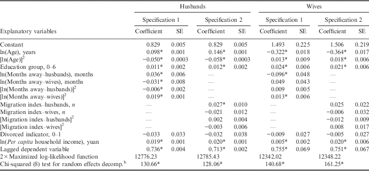
Table 3 presents the results from estimating dynamic random effects models for self-reported health of husbands and wives. Specifications 1 and 2 included, respectively, the number of months that husbands and wives were away from home and the migration index. Coefficients of individuals’ age and its square were estimated with opposite signs for husbands and wives and were statistically significant. Second, in Specification 1 for men, there were non-linearities with respect to numbers of months that husbands and wives spent away from home. Coefficient of husband’s time spent away was positive, whereas its square was estimated with a negative coefficient. By contrast, coefficient of wives’ time spent away in Specification 1 was negative, while its square was estimated with a positive coefficient; all coefficients were statistically significant. Because self-reported health status ranged from 1 to 4, the points of inflexion with respect to months away were not computed and are illustrated below for blood pressures.
Maximum likelihood estimates of dynamic random effects models for self-reported health of husbands and wives using four time observations from the China Health and Nutrition Surveys, 1997–2006Footnote a

a Slope coefficients and standard errors are reported for 3622 husbands and wives in the balanced panel; dynamic models were estimated by maximum likelihood. Higher values of self-reported health reflect better health status.
b Chi-squared (8) statistics for testing validity of the simple random effects decomposition in equation (2).
*p<0.05.
Third, in Specification 1 for wives, the coefficient of husbands’ time spent away from home was negatively and significantly associated with self-reported health. While the coefficient of months that wives were away was not a significant predictor of their self-reported health in Specification 1, its square was estimated with a positive and significant coefficient. In contrast to these findings, the coefficient of migration index was significant only in Specification 2 for husbands; coefficients of this variable and its square were not statistically significant in the remaining models in Table 3.
Fourth, coefficients of the indicator variables for whether husbands and wives divorced during 1997–2006 were estimated with negative signs but were not statistically different from zero. Thus, divorce did not have a significant impact on self-reported health status. Fifth, coefficients of per capita household incomes were estimated with positive signs and were statistically significant in all models in Table 3. Also, coefficients of the lagged dependent variables were in the neighbourhood of 0.75. Thus, the long-run effects of explanatory variables on self-reported health status were four times as large in magnitude. For example, while the short-run impact of per capita household income on husbands’ self-reported health in Specification 1 was 0.02, the long-run impact was 0.08. Lastly, likelihood ratio statistics indicated that the data for husbands and wives should not be pooled. Moreover, the simple random effects model in equation (2) was rejected using likelihood ratio statistics reported in Table 3. The errors affecting the model for self-reported health were likely to be serially correlated, and the maximum likelihood estimation methods tackled such problems.
Husbands’ and wives’ blood pressures
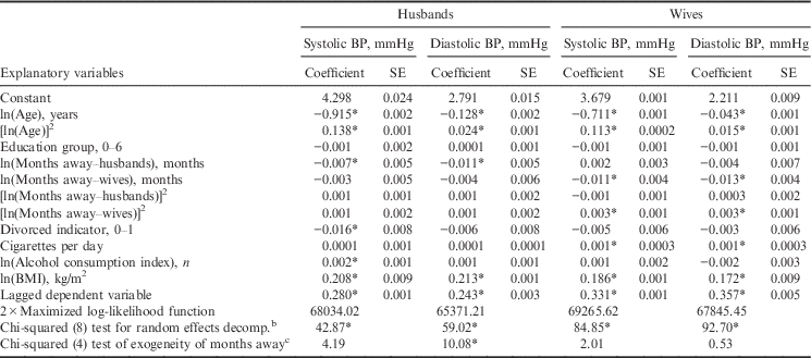
Table 4 presents the results from models for systolic and diastolic blood pressures of husbands and wives. There were non-linearities apparent with respect to age in systolic and diastolic blood pressures. For example, derivatives of husbands’ and wives’ systolic blood pressures were zero at ages 33.71 and 23.25 years, respectively. Thus, wives started experiencing increases in systolic blood pressure at earlier ages. Similarly, the point of inflexion of diastolic blood pressure with respect to age was lower for wives.
Maximum likelihood estimates of dynamic random effects models for systolic and diastolic blood pressures of husbands and wives using four time observations from the China Health and Nutrition Surveys, 1997–2006Footnote a

a Slope coefficients and standard errors are reported for 3662 husbands and wives in the balanced panel; dynamic models were estimated by maximum likelihood.
b Chi-squared (8) statistics for testing validity of the simple random effects decomposition in equation (2).
c Test for null hypothesis that husbands’ (wives’) months away were correlated with random effects using deviations from the time means of explanatory variables as instrumental variables.
*p<0.05.
Second, the numbers of months husbands were away from home were negatively and significantly associated with their systolic and diastolic blood pressures; the coefficient of the square of this variable was not statistically different from zero. The numbers of months that wives were away from home were not significant predictors of husbands’ blood pressures. These findings contrast with the significant associations between husbands’ self-reported health and number of months their wives were away and its square in Table 3. Further, in the models for wives’ systolic and diastolic blood pressures, numbers of months that wives were away were estimated with significant negative coefficients, whereas its square had positive and significant coefficients. Thus, wives’ blood pressure levels declined with the durations away from home and the inflexion points were reached at 6.25 and 8.73 months, respectively, for systolic and diastolic blood pressures.
Third, the coefficients of indicator variable for divorce during 1997–2006 were estimated with negative signs in the models for systolic and diastolic blood pressures of husbands and wives. However, the coefficient was statistically different from zero only in the model for husbands’ systolic blood pressure. These findings suggest that divorce did not have adverse effects for individuals’ health reflected in blood pressures thereby supporting the results from models for self-reported health in Table 3. The negative and significant effect of divorce for husbands’ systolic blood pressure provided some support for the third hypothesis that divorce might have lowered domestic tension for couples in tense marriages.
Fourth, coefficients of numbers of cigarettes smoked were positive in the models for systolic and diastolic blood pressures of husbands and wives. However, the coefficients were statistically different from zero only in the models for wives. These results suggest that despite fewer wives smoking cigarettes, women were more likely to be adversely affected by smoking. Furthermore, the index of alcohol consumption was positively and significantly associated with husbands’ systolic blood pressure; wives’ alcohol consumption index was not significantly associated. Fifth, the BMIs of husbands and wives were positively and significantly associated with their systolic and diastolic blood pressures. The short-run elasticities of systolic blood pressure with respect to BMI for husbands and wives were 0.21 and 0.19, respectively; the corresponding long-run elasticities were 0.29 and 0.27, respectively.
Lastly, the null hypotheses that the random effects affecting the model for systolic and diastolic blood pressures of husbands (wives) were correlated with the number of months for which husbands (wives) were away from home were tested in linear versions of the models using likelihood ratio test statistics. The test statistics for the systolic blood pressure of husbands and wives in Table 4 were 4.19 and 2.01, respectively, thereby not rejecting the null hypotheses. The test statistics in the model for diastolic blood pressures of husbands and wives were 10.08 and 0.53, respectively. The null hypothesis was rejected for men’s diastolic blood pressure indicating that health might have played a role in determining the months for which husbands were away from home. The estimated model parameters were similar in the two models where the number of months was treated as uncorrelated with the random effects and where it was assumed to be correlated.
Discussion
This paper presents comprehensive analyses of nine waves of longitudinal data from the China Health and Nutrition Surveys during 1989–2011, focusing on the effects of internal migration on the chances of marital dissolution and for health and well-being indicators. Previous analyses have not postulated dynamic formulations for individuals’ self-reported health and blood pressures. First, the numbers of months that husbands and wives spent away from home significantly increased their respective chances of marital dissolution. This may have been partly due to greater socializing opportunities in urban areas. The periods for which the spouses of the migrants were away were not significant predictors of marital dissolution. This was presumably because of the different effects of explanatory variables for husbands and wives and also because the parameters were estimated using ‘unbalanced panels’. If, for example, ‘balanced panel’ data were analysed for couples who were initially married and may have divorced before the next time period, then the durations for which husbands and wives were away might have had similar effects on the chances of divorce. To understand the effects of migration on family dynamics, it would be useful to compile data on numbers of months that husbands and wives spend away from home and on their hours of labour supply to assess their work efforts.
Second, the results in Table 2 show that there was son preference among husbands; the inability to have more children under the one-child policy increased the chances of marital dissolution. For example, of the 113 men who re-married in the sample, 66 had only daughters, i.e. 58.4% of divorced men with only daughters re-married. The corresponding figure for women was 44.5% and the difference was statistically significant. Thus, the recent relaxation of the one-child policy in China may not significantly increase the ratio of girls to boys if men without sons re-marry with the expectation of producing a male child. Third, in view of the fact that the divorce rates were below 5% even in 2011, it is likely that divorce occurred mainly in extenuating circumstances such as in tense and abusive marriages. The Marriage Law amendment of 2001 indicator variable was invariably estimated with positive and significant coefficients in Table 2 indicating the benefits of the amendment for women’s rights.
Fourth, dynamic random effects models for husbands’ and wives’ self-reported heath provided useful insights. The coefficient of the indicator variable for whether the individual divorced during 1997–2006 was not statistically different from zero indicating that divorce did not lower self-reported health. Fifth, because self-reported health is likely to reflect multiple dimensions, the models for blood pressures provided substantive insights into the effects of migration durations. For example, the models for wives’ systolic and diastolic blood pressures in Table 4 showed significant effects of the numbers of months away from home; wives’ systolic and diastolic blood pressures increased if they were away for longer than 6.25 and 8.73 months, respectively. Thus, family-friendly leave policies for migrant workers are likely to enhance their health status. Furthermore, the significant negative effect of divorce on husbands’ systolic blood pressure indicated that divorce might have lowered the tension for men in tense marriages. It would therefore be prudent not to extol the benefits of marriage for health in China since divorce seems a sensible option for irreconcilable couples.
Finally, exogeneity hypotheses for number of months that husbands and wives were away from home could not be rejected using likelihood ratio tests in the models for husbands’ systolic blood pressure and wives’ systolic and diastolic blood pressures. The null hypothesis was rejected in the model for husbands’ diastolic blood pressure indicating that men with lower diastolic blood pressure may have been able to spend more time working away from home. These findings suggest the importance of health status for migrants’ labour supply. It would be helpful for migrants with their hukou in rural China to have access to health care in places of employment to enhance their health status and labour productivity.
Acknowledgments
This paper extends the findings from a chapter in Xiayun Tan’s PhD dissertation. The revisions of the paper have benefited from the helpful comments of a reviewer and the Editor.