
I. INTRODUCTION
Graphene has become a topic of intense research in recent years due to the unique electronic, optical, and mechanical properties it possesses. Although being transparent in the visible region, the collective oscillation of charge carriers of graphene in the terahertz regime enables supporting surface plasmon polaritons (SPPs), confining the light into subwavelength dimensions. Reference Grigorenko, Polini and Novoselov1 The plasmonic efficiency of graphene is considerably higher than that of noble metals in the visible light range because of lower loss, Reference Jablan, Buljan and Soljačić2 higher confinement factors, Reference Woessner, Lundeberg, Gao, Principi, Alonso-González, Carrega, Watanabe, Taniguchi, Vignale, Polini, Hone, Hillenbrand and Koppens3 and minimal out-of-plane scattering of SPPs. Reference Inampudi and Mosallaei4 Moreover, the plasmonic modes of graphene can be tuned by adjusting its chemical potential through external stimuli such as gate-biasing Reference Wang, Zhang, Tian, Girit, Zettl, Crommie and Shen5 and intense magnetic fields. Reference Zhang, Jiang, Small, Purewal, Tan, Fazlollahi, Chudow, Jaszczak, Stormer and Kim6 On account of these features, graphene provides a great platform for optoelectronic applications as an alternative to other plasmonic materials. It has been extensively exploited for a variety of optical applications such as cloaking, Reference Chen and Alù7 solar cells, Reference Miao, Tongay, Petterson, Berke, Rinzler, Appleton and Hebard8 imaging devices, Reference Inampudi, Cheng and Mosallaei9–Reference Forouzmand, Bernety and Yakovlev11 optical antennas, Reference Cheng, Jafar-Zanjani and Mosallaei12,Reference Jafar-Zanjani, Cheng and Mosallaei13 and metasurfaces. Reference Cheng, Wang, Mosallaei and Kaxiras14,Reference Li, Yao, Xia, Shen, Tian and Liu15
Meanwhile, graphene, being only one atom thick, offers unique mechanical properties such as very low mass density (1.5–2 g/cm3), high elastic strength (∼130 GPa), Reference Lee, Wei, Kysar and Hone16 exceptionally stiff in-plane Young’s modulus (∼1 TPa), Reference Tsoukleri, Parthenios, Papagelis, Jalil, Ferrari, Geim, Novoselov and Galiotis17 strong adhesion, and flexibility. Reference Jiang, Wang and Li18–Reference Bunch and Dunn20 These properties can be harnessed in nanomechanical devices such as for high-sensitivity force/mass detectors Reference Chen, Rosenblatt, Bolotin, Kalb, Kim, Kymissis, Stormer, Heinz and Hone21 and tunable mechanical oscillators. Reference Chen, Lee, Deshpande, Lee, Lekas, Shepard and Hone22,Reference Barton, Storch, Adiga, Sakakibara, Cipriany, Ilic, Wang, Ong, McEuen, Parpia and Craighead23
Recently, motivated by its unique optical and mechanical properties, graphene has been explored for optomechanical applications through mechanical actuation of graphene sheets using optical forces. Reference Mousavi, Rakich and Wang24–Reference Zhang, Shen, Koschny and Soukoulis28 Following the pioneer work by Ashkin, Reference Ashkin29 the use of optical forces has been investigated for manipulating and trapping microscopic objects Reference Shvedov, Rode, Izdebskaya, Desyatnikov, Krolikowski and Kivshar30 as well as pressurizing and deforming thin-film structures. Reference Soo, Ji, Jae and Sang31 In this context, the major challenge is the notoriously weak nature of optical forces. As such, several research efforts have been put into identifying the routes for enhancing the optical forces by leveraging enhanced light–matter interactions without the need to increase the optical power. Reference Woolf, Loncar and Capasso32–Reference Salary and Mosallaei40
Optical forces can be categorized into two different types based on their origin, namely, radiation pressure and gradient forces. Reference Salary and Mosallaei40 Radiation pressure is a result of exchange of linear momentum between a photon (momentum hω/c) and the object upon scattering or absorption of light. Thus, the transverse optical force exerted on planar surface illuminated by an optical power P is F = P/c in case of total absorption and F = 2P/c in case of total reflection. Reference Rodriguez, McCauley, Hui, Woolf, Iwase, Capasso, Loncar and Johnson35 The gradient forces are due to the evanescent bonding between light waves and can arise from the in homogeneities in light intensity created by the structured light illumination or evanescent interaction between localized optical modes. Reference Woolf, Loncar and Capasso32–Reference Rodriguez, McCauley, Hui, Woolf, Iwase, Capasso, Loncar and Johnson35
Generally, there exists two optical force enhancement mechanisms. The first mechanism is exploiting Fabry–Perot resonances excited in layered structures. The Fabry–Perot will increase the reflectivity from the object which leads to enhancement of radiation pressure for a given optical power. Such enhanced forces have been observed in the Fabry–Perot cavities formed between a suspended graphene above a substrate with high reflectivity which can lift the graphene away into a series of equilibrium heights above the substrate. Reference Mousavi, Rakich and Wang24 The second mechanism relies on the excitation of guided modes in a layered structure which enables resonant increase in the field intensity gradient accompanied by a significant enhancement of gradient optical forces. This effect has been exploited in plasmonic waveguides formed by two coupled parallel plasmonic slabs such as gold and silicon carbide for inducing large optical forces. Reference Woolf, Loncar and Capasso32,Reference Li, Lawandy and Zia33 In this case, the sign of the interaction is controlled by the relative phase of the guided modes in the waveguides and can lead to repulsive or attractive forces corresponding to symmetric and asymmetric modes. More recently, the same phenomenon has been demonstrated between two parallel graphene sheets or nanoribbons. Reference Salary, Inampudi, Zhang, Tadmor and Mosallaei25–Reference Zhang, Shen, Koschny and Soukoulis28 It has been observed that the induced optical forces in graphene waveguides are considerably larger (∼3 orders of magnitude) comparing to the plasmonic metal counterparts which is attributed to the lower loss and higher SPP confinement in graphene layers. Furthermore, moving from a three-dimensional structure to a two-dimensional (2D) sheet is expected to magnify the effect of the force in terms of the resulting deformation and accelerations. Reference Salary, Inampudi, Zhang, Tadmor and Mosallaei25
The 2D layers of graphene can be integrated into a multilayer stack (vertical 2D heterostructure). Reference Yu, Li, Zhou, Chen, Wang, Huang and Duan41,Reference Batrakov, Kuzhir, Maksimenko, Paddubskaya, Voronovich, Lambin, Kaplas and Svirko42 The resulting 2D structures provide access to a spectrum of guided modes enriching the optomechanical phenomena and offering a new route for tailoring optical forces and mechanical states in the graphene systems. In this article, we study the optomechanical interactions in layered stacking of graphene sheets and resolve different mechanical states of such systems. We demonstrate the dependence of the induced optical forces to the interlayer spacing and the chemical potential of the sheets. Our results can be of great benefit in designing new optomechanical platforms using graphene layers for a variety of applications such as all-optical tunable filters, switches, modulators, and actuators. The rest of this article is organized as follows. In Sec. II, we briefly discuss the theoretical framework for calculation of guided modes in layered graphene systems and the corresponding optical forces, which is based on a combination of the scattering matrix approach and Maxwell stress tensor method. In Sec. III, the optomechanical modes in coupled multilayer systems of graphene sheets are characterized, and the results are discussed. The conclusion is drawn in Sec. IV.
II. METHODS
In this work, we use an approach based on scattering matrix technique Reference Inampudi, Nazari, Forouzmand and Mosallaei43 to characterize the eignemodes and obtain the corresponding electromagnetic fields in a multilayer stack of 2D sheets. Following the calculation of electromagnetic fields in each layer, we obtain the optical pressure exerted on graphene sheets based on Maxwell stress tensor formulation. Reference Kemp, Grzegorczyk and Kong44
A. Scattering matrix approach
Consider a vertical multilayer stack of graphene sheets suspended in free-space with the l-th layer having the surface conductivity of σ
l
and sitting at z = z
l
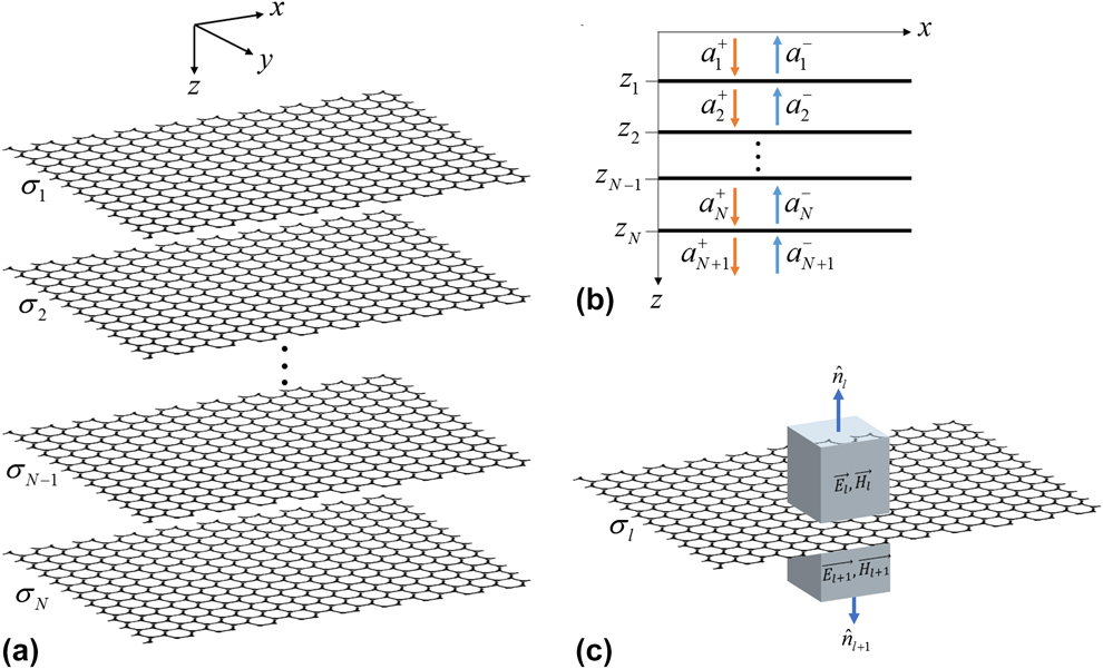
as shown in Fig. 1(a). We assume that the structure is infinitely extended in the x–y plane which is a fair assumption when the dimensions of the sheets are large compared with the wavelength. The electromagnetic fields in such a layered structure can be expressed as a combination of transverse electric (TE) and transverse magnetic (TM) modes. Here, we only consider TM modes which enable surface plasmon excitation in the near- and mid-infrared regimes. In this case, the total electric and magnetic field components associated with each layer, represented as
 ${\vec{E}_l}$
and
 ${\vec{H}_l}$
, can be written as integrals of modal components propagating in the forward (+z) and backward (−z) directions
Reference Inampudi, Nazari, Forouzmand and Mosallaei43
:
 $${\vec{E}_l} = \int_{ - \infty }^\infty {\int_{ - \infty }^\infty {\left[ {{a^{\left( l \right) + }}{{\vec{E}}^{\left( l \right) + }}{\Phi ^{\left( l \right) + }} + {a^{\left( l \right) - }}{{\vec{E}}^{\left( l \right) - }}{\Phi ^{\left( l \right) - }}} \right]} } {\rm{d}}{k_x}{\rm{d}}{k_y}\quad ,$$
 $${\vec{H}_l} = \int_{ - \infty }^\infty {\int_{ - \infty }^\infty {\left[ {{a^{\left( l \right) + }}{{\vec{H}}^{\left( l \right) + }}{\Phi ^{\left( l \right) + }} + {a^{\left( l \right) - }}{{\vec{H}}^{\left( l \right) - }}{\Phi ^{\left( l \right) - }}} \right]} } {\rm{d}}{k_x}{\rm{d}}{k_y}\quad .$$
(a) The schematic of a multilayer graphene stack suspended in free space. (b) The modal spectrum in the layered structure. (c) The integration path chosen for evaluating the flux of Maxwell stress tensor to calculate the optical force on a graphene sheet.

The modal spectrum in the layered structure is shown schematically in Fig. 1(b). Each mode is characterized by transverse wavevector components {k
x
, k
y
} that are conserved in each layer. The quantities a
(l)± are unknown amplitudes corresponding to the modes propagating in the l-th layer;
 ${\vec{E}^{\left( l \right) \pm }}$
and
 ${\vec{H}^{\left( l \right) \pm }}$
denote electric and magnetic field modal profiles in the l-th layer, respectively; and
 ${\Phi ^{\left( l \right) \pm }} = \exp \left( {i{k_x}x + i{k_y}y \pm ik_z^{\left( l \right)}z} \right)$
represent the phase factors of the modes in the l-th layer. In all the above quantities, the (+) sign denotes the modes traveling in the forward direction and the (−) sign represents the modes traveling in the backward direction. The modal field profiles in each layer can be expressed analytically as:
 $$\vec{E}_p^{\left( l \right) \pm } = {{\left\{ { \mp {{k_z^{\left( l \right)}{k_x}} \over {{\varepsilon _{\left( l \right)}}}}, \mp {{k_z^{\left( l \right)}{k_y}} \over {{\varepsilon _{\left( l \right)}}}},{{k_\rho ^2} \over {{\varepsilon _{\left( l \right)}}}}} \right\}} / {{k_0}{k_\rho }}}\quad ,$$
 $$\vec{H}_p^{\left( l \right) \pm } = {{\left\{ {{k_y}, - {k_x},0} \right\}} / {{k_\rho }\quad ,}}$$
where k
0 = ω/c,
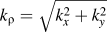 ${k_\rho } = \sqrt {k_x^2 + k_y^2}$
, and
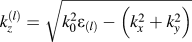 $k_z^{\left( l \right)} = \sqrt {k_0^2{\varepsilon _{\left( l \right)}} - \left( {k_x^2 + k_y^2} \right)}$
.
For each mode, only two of the amplitudes a (l)± in the layered structure are independent and the rest of the amplitudes can be related to each other through the scattering matrix equations enforcing the boundary conditions. The scattering matrix equation associated with the l-th interface can be expressed as:
 $$\left[ {\matrix{ {{a^{\left( l \right) - }}} \cr {{a^{\left( {l + 1} \right) + }}} \cr} } \right] = \left[ {\matrix{ {{\Phi ^{\left( l \right) + }}} 0 \cr 0 {{\Phi ^{\left( {l + 1} \right) - }}} \cr} } \right]\left[ {\matrix{ {{r^{\left( l \right) + }}} {{t^{\left( l \right) - }}} \cr {{t^{\left( l \right) + }}} {{r^{\left( l \right) - }}} \cr} } \right]\left[ {\matrix{ {{\Phi ^{\left( l \right) + }}} 0 \cr 0 {{\Phi ^{\left( {l + 1} \right) - }}} \cr} } \right]\left[ {\matrix{ {{a^{\left( l \right) + }}} \cr {{a^{\left( {l + 1} \right) - }}} \cr} } \right]\quad ,$$
where Φ(l)± are calculated at z = z l , and the reflection/transmission coefficients can be calculated as:
 $${r^{\left( l \right) + }} = {{k_z^{\left( l \right)}{\varepsilon _{\left( {l + 1} \right)}} - k_z^{\left( {l + 1} \right)}{\varepsilon _{\left( l \right)}} + k_z^{\left( l \right)}k_z^{\left( {l + 1} \right)}{\sigma _{\left( l \right)}}{\eta _0}} \over D}\quad ,$$
 $${r^{\left( l \right) - }} = {{k_z^{\left( {l + 1} \right)}{\varepsilon _{\left( l \right)}} - k_z^{\left( l \right)}{\varepsilon _{\left( {l + 1} \right)}} + k_z^{\left( l \right)}k_z^{\left( {l + 1} \right)}{\sigma _{\left( l \right)}}{\eta _0}} \over D}\quad ,$$
 $${t^{\left( l \right) + }} = {{2k_z^{\left( l \right)}{\varepsilon _{\left( {l + 1} \right)}}} \over D}\quad ,$$
 $${t^{\left( l \right) - }} = {{2k_z^{\left( {l + 1} \right)}{\varepsilon _{\left( l \right)}}} \over D}\quad ,$$
where η0 is the wave impedance of free-space and
 $$D = k_z^{\left( l \right)}{\varepsilon _{\left( {l + 1} \right)}} + k_z^{\left( {l + 1} \right)}{\varepsilon _{\left( l \right)}} + k_z^{\left( l \right)}k_z^{\left( {l + 1} \right)}{\sigma _{\left( l \right)}}{\eta _0}\quad .$$
As such, the relation between the fields in any two layers can be obtained through multiplication of consecutive scattering matrices which can yield the total reflection and transmission of the layered system.
The singular solutions of the system (poles of the reflection coefficient) correspond to the zero incident fields
 $\left( {a_1^ + = 0,\quad a_{N + 1}^ - = 0} \right)$
and non-zero scattered field
 $\left( {a_1^ - \ne 0,\quad a_{N + 1}^ + \ne 0} \right)$
which characterize the guided modes of the multilayer stack.
The conductivity of graphene in the THz regime can be expressed by a Drude model as Reference Inampudi, Nazari, Forouzmand and Mosallaei43 :
 $$\sigma \left( \omega \right) = {{{e^2}{v_{\rm{f}}}} \over {{\varepsilon _0}c\pi \hbar }}{{\sqrt {\pi {n_{\rm{s}}}} } \over {{1 / \tau } - i\omega }}\quad ,$$
where v f is the Fermi velocity, τ is the relaxation time, and n s denotes the surface carrier concentration. The Fermi velocity and relation time are chosen as v f = 106 m/s and τ = 500 fs, based on the experimentally obtained values. Reference Woessner, Lundeberg, Gao, Principi, Alonso-González, Carrega, Watanabe, Taniguchi, Vignale, Polini, Hone, Hillenbrand and Koppens3 The surface carrier concentration can be tuned in the range of 1016–1018 m−2 by using external stimuli. Reference Efetov and Kim45 In this work n s = 6.37 × 10¹⁶ m−2 is chosen in accordance with Woessner et al., Reference Woessner, Lundeberg, Gao, Principi, Alonso-González, Carrega, Watanabe, Taniguchi, Vignale, Polini, Hone, Hillenbrand and Koppens3 unless specified otherwise.
B. Maxwell stress tensor method
Once the electromagnetic fields in each layer are calculated, the time-averaged optical force exerted on each graphene sheet can be calculated by evaluating the flux of Maxwell stress tensor as Reference Kemp, Grzegorczyk and Kong44 :
 $${\vec{F}_l} = - {1 \over 2}{\mathop{\rm Re}\nolimits} \left\{ {\oint_{{S_l}} {{\rm{d}}S\left[ {\hat{n}.\overline{\overline T} \left( {\vec{r}} \right)} \right]} } \right\}\quad ,$$
where S l is the integration path enclosing the surface of l-th graphene sheet. The complex Maxwell stress tensor is expressed in terms of the electromagnetic fields as:
 $$\overline{\overline T} \left( {\vec{r}} \right) = {1 \over 2}\left( {\vec{D} \cdot {{\vec{E}}^ * } + {{\vec{B}}^ * } \cdot \vec{H}} \right)\overline{\overline I} - \vec{D}{\vec{E}^ * } - {\vec{B}^ * }\vec{H}\quad ,$$
where
 $\overline{\overline I}$
is the 3 × 3 identity matrix and asterisk (*) denotes the complex conjugate. By choosing the integration path around the infinitesimal segments of the graphene sheet as shown in Fig. 1(c), we are able to calculate the force per unit area or pressure in terms of the electromagnetic fields at the interface in the below and above layers of the graphene sheet:
 $${\vec{F}_l} = {1 \over 2}{\mathop{\rm Re}\nolimits} \left\{ {\hat{z} \cdot \overline{\overline T} \left( {z = {z_l}^ - } \right) - \hat{z} \cdot \overline{\overline T} \left( {z = {z_l}^ + } \right)} \right\}\quad ,$$
where:
 $$\eqalign{ \hat{z} \cdot \overline{\overline T} \left( {z = {z_l}^{ + , - }} \right) = \hat{z}\left[ {{{{\varepsilon _{l + 1,l}}} \over 2}\left( {{{\left| {{E_x}\left( {z = {z_l}^{ + , - }} \right)} \right|}^2} + {{\left| {{E_y}\left( {z = {z_l}^{ + , - }} \right)} \right|}^2} - {{\left| {{E_z}\left( {z = {z_l}^{ + , - }} \right)} \right|}^2}} \right)} \right. \cr \left. { - {{{\mu _{l + 1,l}}} \over 2}\left( {{{\left| {{H_x}\left( {z = {z_l}^{ + , - }} \right)} \right|}^2} + {{\left| {{H_y}\left( {z = {z_l}^{ + , - }} \right)} \right|}^2} - {{\left| {{H_z}\left( {z = {z_l}^{ + , - }} \right)} \right|}^2}} \right)} \right] \cr + \hat{x}\left[ { - {\varepsilon _{l + 1,l}}{E_z}\left( {z = {z_l}^{ + , - }} \right)E_x^ * \left( {z = {z_l}^{ + , - }} \right) - {\mu _{l + 1,l}}{H_z}\left( {z = {z_l}^{ + , - }} \right)H_x^ * \left( {z = {z_l}^{ + , - }} \right)} \right] \cr + \hat{y}\left[ { - {\varepsilon _{l + 1,l}}{E_z}\left( {z = {z_l}^{ + , - }} \right)E_y^ * \left( {z = {z_l}^{ + , - }} \right) - {\mu _{l + 1,l}}{H_z}\left( {z = {z_l}^{ + , - }} \right)H_y^ * \left( {z = {z_l}^{ + , - }} \right)} \right]\quad . \cr}$$
As such, the knowledge of the electromagnetic fields in the layered system can give us the optical pressure exerted on each graphene sheet.
III. RESULTS
In this section, we characterize the eigenmodes of layered graphene systems and demonstrate mechanical states corresponding to each mode. There are two schemes to excite coupled resonances on the graphene sheets depending on whether the incident power comes in the form of external radiation or a guided mode. In the former case, near-field coupling is achieved by a sharpened metallic tip or tapering metal aperture above the sheets. Such sources can be modeled by a dipole, exciting all the evanescent modal spectrum. In the latter technique, a specific evanescent mode can be excited by diffraction from a grating, coupling to a prism, or another waveguide. This excitation scheme offers the opportunity to selectively couple to one of the eigenmodes of the layered system and gives a better control over the mechanical state of the graphene sheets.
Reference Salary, Inampudi, Zhang, Tadmor and Mosallaei25
Here, we focus on the guided mode excitation. The eigenmodes of the layered system are obtained based on the scattering matrix approach. To obtain the mode profile and the exerted optical forces on the graphene sheets corresponding to each mode, the guided mode is excited from the side and propagated parallel to the graphene sheets through a mode-matching technique.
Reference Inampudi and Mosallaei4
Referring to the coordinate system shown in Fig. 1(a), the TM-guided modes are launched along the y-axis from the side which can exert a transverse optical force F
z
to the sheets. Each guided mode is characterized by the field components {H
y
, E
x
, E
z
} and satisfies the dispersion relation
 $k_0^2 = k_x^2 - k_z^2$
.
As implied by Eqs. (14) and (15), the optical pressure is linearly proportional to the field intensity or input optical power. The optical power flowing in the propagation direction of a guided mode in a layered system can be obtained, per unit width of the sheets as Reference Salary, Inampudi, Zhang, Tadmor and Mosallaei25 :
 $$\eqalign{\displaylines{ P = {{{P_z}} \over W} = {1 \over 2}{\mathop{\rm Re}\nolimits} \left\{ {\int_{ - \infty }^{ + \infty } {\vec{E} \times {{\vec{H}}^ * }{\rm{d}}z} } \right\} }\cr {= {\mathop{\rm Re}\nolimits} \left\{ {{{{k_z}} \over {\omega {\varepsilon _0}}}} \right\}\int_0^{ + \infty } {{{\left| {{H_y}} \right|}^2}{\rm{d}}z} \quad . \cr}$$
In the following, all the results are presented assuming the optical power flowing in the propagation direction per unit width distributed along the layered system of graphene sheets is 1 mW/μm.
To characterize the optomechanical modes of a layered system according to the mode profile, we define the real part of the TE field component E x as mode profile which is continuous across the interfaces and matches the charge distribution across the sheets which determines the repulsive/attractive nature of the optical force. Reference Woolf, Loncar and Capasso32
A. Two-layer graphene systems
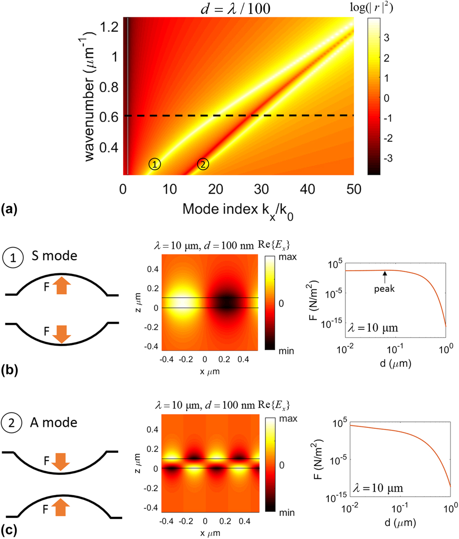
We start by the simplest structure consisted of two parallel graphene sheets. Figure 2(a) shows the dispersion curve of SPP modes of two coupled graphene sheets separated by a distance of d = λ/100. The dispersion curves are represented by plotting the intensity of reflection coefficient of the layered system in logarithmic scale (log(|r|2)) in (k 0, k x ) space. Two coupled modes can be identified for this system. For the large wavenumbers (short wavelengths) the modes are degenerate. Increasing the wavelength breaks the degeneracy of the SPP modes, and the eigenvalues of the propagation constant of the modes (k SPP) become well separated. It should be noted that k SPP also depends on the separation distance of the graphene sheets. When the separation between the layers is not small enough compared with the wavelength, the coupling between the sheets is negligible and the modes become degenerate. Bringing the sheets closer, leads to stronger coupling between the sheets and breaks degeneracy of the modes.
(a) The dispersion curves of a two-layer graphene system with a separation distance of d = λ/100. The dashed line corresponds to the excitation wavelength of λ = 10 μm. (b) and (c) The mechanical states, mode profiles, and dependence of induced pressure on the separation distance between the sheets, corresponding to each guided mode. The solid lines in the nearfield plots denote the graphene sheets. The order of the modes is shown in circles. The first mode is a symmetric mode denoted by “S” and the second mode is an asymmetric mode denoted by “A”.
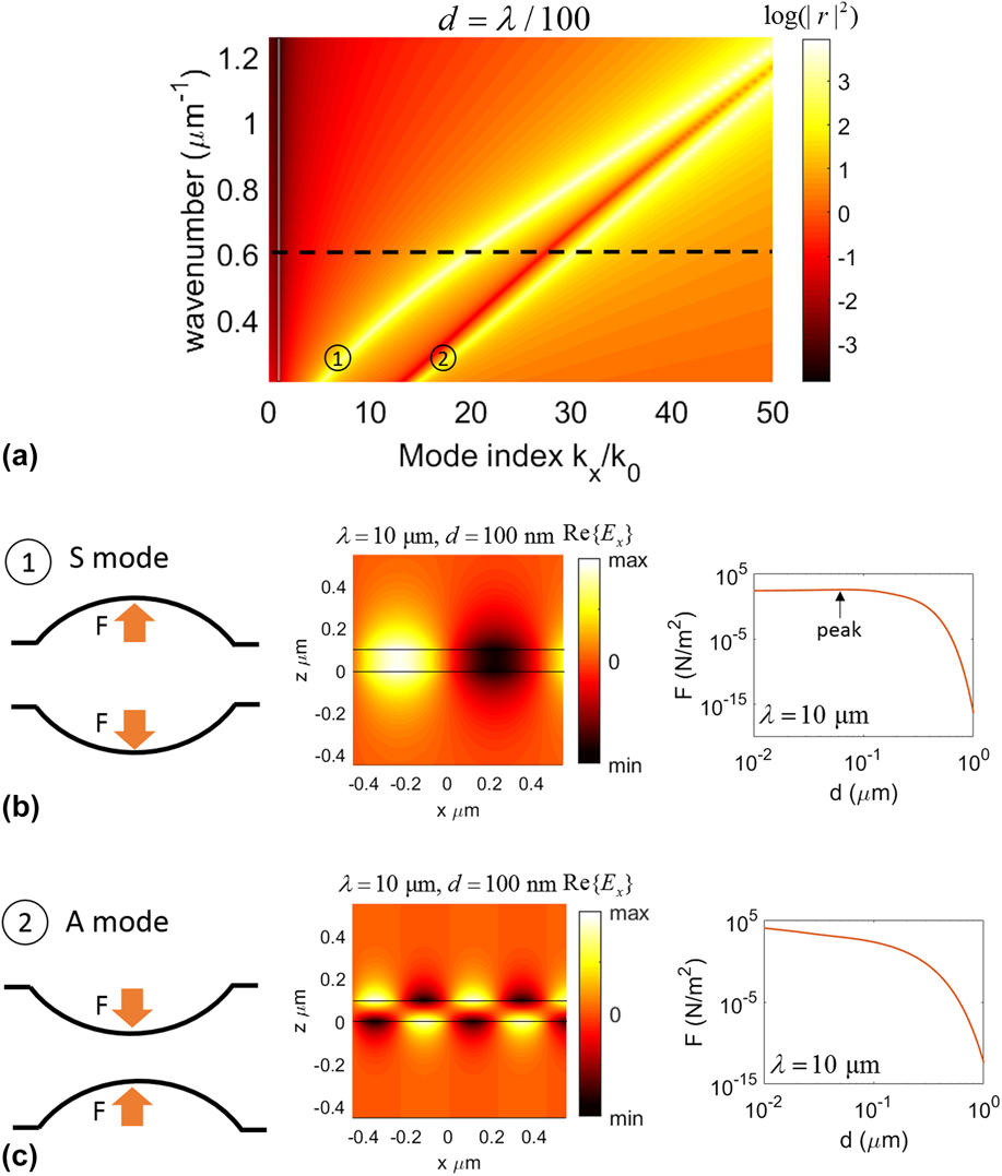
Figures 2(b) and 2(c) show the mode profiles and mechanical states corresponding to the guided modes as well as the dependence of the induced optical pressure magnitudes on the gap distance between the graphene layers at the excitation wavelength of λ = 10 μm. The corresponding wavenumber to this wavelength is denoted by the dashed line in the dispersion diagram [Fig. 2(a)]. It should be noted that in the dispersion plots only the real part of propagation constant k x is considered, while the presented mode profiles and optical forces are calculated using complex-valued wavevectors. The solid lines in the mode profile plots denote the location of the graphene sheets.
As it can be seen, for the first mode E x has an even parity, whereas in the second mode, it has an odd parity. The modes with even and odd parities are referred to as symmetric and asymmetric modes, respectively. Reference Salary, Inampudi, Zhang, Tadmor and Mosallaei25 These modes are characterized with repulsive and attractive forces between the sheets as shown by the mechanical states in Fig. 2. The relative phase of the mode profiles provides an intuition into the repulsive/attractive nature of the induced optical forces as it follows the charge distribution across the graphene sheets. In the symmetric mode, E x is in-phase across the two sheets resulting into a repulsive force, whereas in the asymmetric mode, E x is out-of-phase across the sheets inducing an attractive force between them.
The dependence of the attractive and repulsive pressures on the separation distance between the sheets can be studied in two coupling regimes. For the small separation distances (strong coupling regime), the asymmetric mode produces significantly larger pressures than the symmetric counterpart. This can be justified by observing that the asymmetric mode is settled further from the light line (k x /k 0 = 1) in the dispersion diagram implying a stronger localization of SPPs which leads to a much larger field gradient and optical force as well. In this regime, the attractive force shows an exponential dependence to the separation distance, whereas the repulsive force is weakly related to the gap distance. For large separation distances (weak-coupling regime), the pressures arising from the symmetric and asymmetric modes have nearly equivalent magnitudes and both show an exponential dependence on the separation distance. Moreover, it can be noticed that the repulsive force induced by the symmetric mode shows an increasing trend in the strong coupling regime reaching a maximum before going into the weak coupling regime (denoted by the arrow), whereas the attractive force which resulted from the asymmetric mode exhibits a monotonic decreasing trend with increasing separation distance.
The induced optical forces can deform the graphene sheets and give rise to concave or convex blisters with a height of several nanometers. Reference Salary, Inampudi, Zhang, Tadmor and Mosallaei25,Reference Xu, Shi, Liu, Wang and Zhang26,Reference Zhang, Shen, Koschny and Soukoulis28 The height of the blisters depends on the optical pressure magnitude as well as dimensions of mechanically clamped graphene sheets; with larger dimensions leading to larger deflections. Reference Salary, Inampudi, Zhang, Tadmor and Mosallaei25
B. Three-layer graphene systems
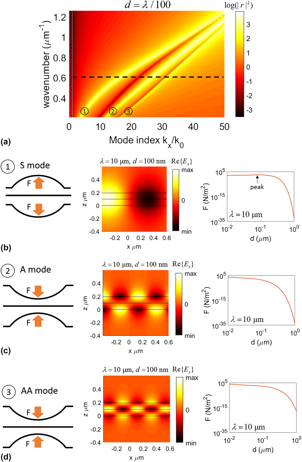
Next, we proceed into a three-layer system. To bring out the essential physics, we consider the separation distance between all layers is the same. Figure 3(a) shows the dispersion curve of SPP modes corresponding to the three-layer system for a gap distance of d = λ/100. One can clearly identify three guided modes from the dispersion diagram which approach degeneracy by increasing the wavenumber (shortening the wavelength).
(a) The dispersion curve of a three-layer graphene system with an equal spacing of d = λ/100. The dashed line corresponds to the excitation wavelength of λ = 10 μm. (b)–(d) The mechanical states, mode profiles, and dependence of induced pressure on the separation distance between the sheets, corresponding to each guided mode. The order of the modes is shown in circles.
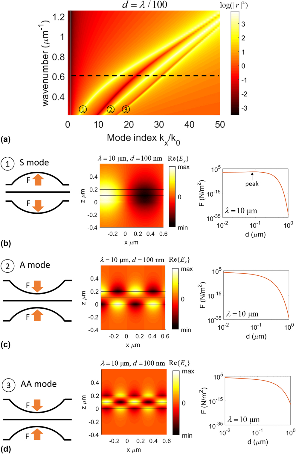
Figures 3(b)–3(d) show the mode profiles and mechanical states corresponding to the guided modes as well as the dependence of the induced optical pressure magnitudes on the interlayer spacing at the excitation wavelength of λ = 10 μm (denoted by the dashed line in the dispersion diagram). Because of the symmetry of the system with respect to excitation (injection of guided mode from the side), the middle layer experiences no optical pressure and remains flat. The profiles of the first and second guided modes closely resemble those of the symmetric and asymmetric modes in a two-layer system, whereas the third guided mode can be viewed as a combination of two asymmetric modes between the consecutive pairs of graphene sheets. Denoting symmetric mode by “S” and asymmetric mode by “A”, the excited guided modes in the three-layer system can be named according to the mode profile in order as: “S”, “A”, and “AA”. The mechanical states of the A and AA modes are the same, whereas the induced optical force by the AA mode is slightly stronger due to the settlement of the mode further away from the light line. Moreover, the magnitudes of the repulsive and attractive forces arising from the symmetric and asymmetric modes are considerably weaker than those of a two-layer system due to the placement of the modes closer to the light line and weaker field gradient. The gap dependence of the repulsive and attractive forces exhibits a similar behavior to that in a two-layer system, with two weak and strong coupling regimes being identified.
C. Four-layer graphene systems
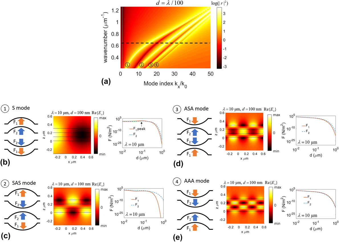
Moving to a four-layer system increases the number of guided modes to four providing access to new mechanical states for the graphene sheets. The dispersion diagram of a four-layer system with equal spacing of d = λ/100 is demonstrated in Fig. 4(a). Four guided modes can be identified which approach degeneracy by increasing the wavenumber. The dispersion diagram also shows the closer settlement of the modes together as the mode indices increase. The mode profiles of each guided mode and the corresponding mechanical states are shown in Figs. 4(b)–4(e) alongside the magnitude of induced optical pressures on each sheet, at the excitation wavelength of λ = 10 μm. In this system, there are two different values for the acting pressure on the graphene sheets which are shown by arrows of different colors.
(a) The dispersion curve of a four-layer graphene system with an equal spacing of d = λ/100. The dashed line corresponds to the excitation wavelength of λ = 10 μm. (b)–(e) The mechanical states, mode profiles, and dependence of induced pressure on the separation distance between the sheets, corresponding to each guided mode. The order of the modes is shown in circles.
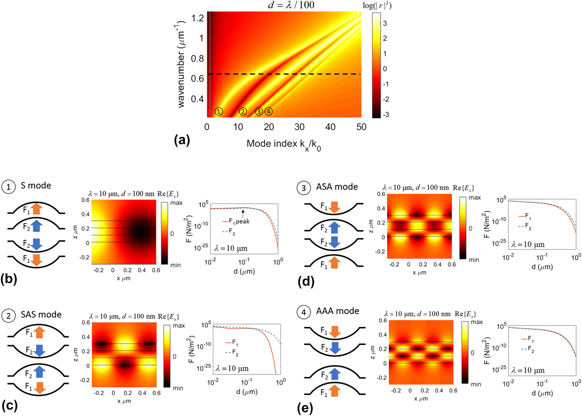
The lowest order mode has a symmetric profile similar to the previous systems, whereas the rest of the modes can be viewed as different combinations of symmetric and asymmetric modes between consecutive pairs of graphene sheets. The four guided modes in the layered system can be named according to their profile in order as: “S”, “SAS”, “ASA”, and “AAA”. The mechanical states corresponding to each mode can be intuitively characterized by observing the relative phase gradient of the field between consecutive pairs of graphene sheets. The gap dependence of the repulsive force arising from the symmetric mode is similar to that in two- and three-layer systems while the force is considerably weaker especially in the weak-coupling regime due to the closer settlement of the mode with respect to the light line. The behavior of attractive forces resulting from AAA and ASA modes with respect to the interlayer spacing follows the same behavior of the attractive force in a two-layer system. The forces arising from the SAS mode show a more complicated behavior with respect to the separation gap, whereas the acting force on the top and bottom layers of the system is significantly diminished in the weak coupling regime.
D. Five-layer graphene systems
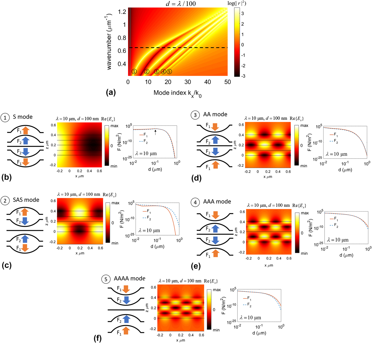
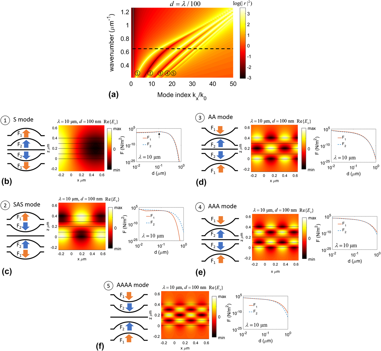
Finally, we consider a five-layer system. The dispersion diagram of such system with equal spacing of d = λ/100 is demonstrated in Fig. 5(a) exhibiting five guided modes being degenerate for large wavenumbers. As the number of modes increases, the separation between modes decreases while the modes with higher indexes approach degeneracy as they are settled close together. The field profiles of each guided mode and the corresponding mechanical states are shown in Figs. 5(b)–5(f) alongside the magnitude of induced optical pressures on each sheet at the excitation wavelength of λ = 10 μm. Similar to the three-layer system, due to the symmetry of the system with respect to excitation and odd number of layers, the middle layer experiences no optical pressure and remains flat. In consistency with the observations made in previous layered systems, the lowest order mode corresponds to a symmetric mode which results in repulsion of all the sheets from the center. The five guided modes in the layered system can be named according to their profile in order as: “S”, “SAS”, “AA”, “AAA”, and “AAAA”. The mechanical states of the AA and AAA modes are the same with the AAA mode inducing slightly larger optical forces due to further distance from the light line and stronger field gradient. The gap dependencies of the arising optical forces closely follow the same behavior in a four-layered system.
(a) The dispersion curve of a five-layer graphene system with an equal spacing of d = λ/100. The dashed line corresponds to the excitation wavelength of λ = 10 μm. (b)–(f) The mechanical states, mode profiles, and dependence of induced pressure on the separation distance between the sheets, corresponding to each guided mode. The order of the modes is shown in circles.
E. Summary
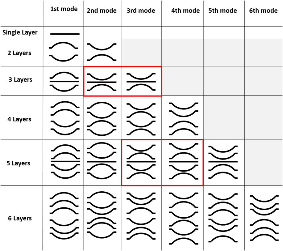
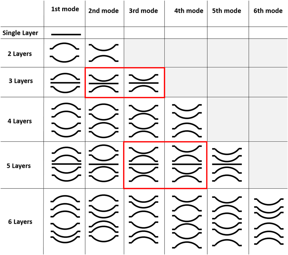
To summarize our observations, the mechanical states corresponding to the excited guided modes in the multilayer stack of graphene sheets up to 6 layers are demonstrated in Fig. 6. The lowest order mode (or fundamental mode) in all layered systems corresponds to a symmetric mode where all the sheets are repulsed from the center. Moreover, the highest order mode in all the systems corresponds to excitation of an asymmetric mode between each consecutive pair of graphene sheets wherein the mechanical state is attraction of all layers toward the center. The mechanical states of layered systems with odd number of layers 2k + 1 is shown to be similar to the states in the system with 2k number of layers, except that the middle layer remains flat and does not experience any optical force due to symmetry with respect to excitation. Moreover, the systems with odd number of layers exhibit a repeated mechanical state in two consecutive modes (shown by the red cells). It should be noted that in the case of external excitation using a dipole source, the middle sheet in the layered system with odd number of layers can also experience an optical force due to the discontinuity of energy across the sheet. In this case, the repulsive/attractive nature of this force depends on the wavelength of the excitation and the cut-off wavevector for the excitation of evanescent modes on the sheet. Reference Salary, Inampudi, Zhang, Tadmor and Mosallaei25 The advantage of multilayer graphene stack can be clearly seen as it provides access to additional guided modes and mechanical states which has the potential for extending the graphene-related optomechanical applications.
The mechanical states corresponding to the guided modes in layered graphene systems. The lowest order mode corresponds to the state wherein all the sheets are repulsed from the center, whereas the highest order mode corresponds to the states in which all the sheets are attracted toward the center.
F. Active tuning
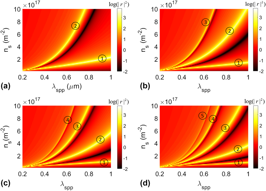
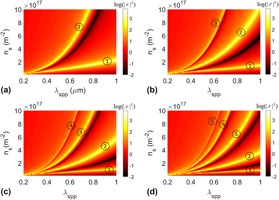
As mentioned in the beginning, the surface carrier concentration of graphene sheets can be tuned in the range of 1016–1018 m−2 through gate-biasing which can yield a variation of 1 order of magnitude in the conductivity. This is a valuable asset offered by graphene which makes it an ideal candidate for tunable optoelectronic and optomechanical applications. For excitation of guided mode in a layered system, a one-dimensional diffraction grating may be used. In this case, the SPP wavelength is determined by the periodicity of the grating λSPP = P. As such, the mechanical state of the layered system is tied to the excited optomechanical mode with a constant SPP wavelength. In this regard, gate-tunability of graphene can be used to adjust the excited optomechanical mode at a certain excitation wavelength which enables the transition between different mechanical states of the system in real-time.
To demonstrate this concept, the dependence of SPP wavelength of optomechanical modes to the surface carrier concentration is shown in Fig. 7 for stack of graphene sheets with different numbers of layers separated by a distance of d = 100 nm at the excitation wavelength λ = 10 μm. The results clearly show that by changing the surface carrier concentration of graphene sheets, it is possible to couple into different optomechanical modes and consequently different mechanical states for a fixed SPP wavelength which is pre-determined by the periodicity of the diffraction grating.
Active tuning of the guided modes propagation wavelength in (a) two-, (b) three-, (c) four-, and (d) five-layer systems of graphene sheets by changing the surface carrier concentration using gate-biasing. This offers a significant advantage for transition between different mechanical states of the system in real-time.
IV. CONCLUSION
In conclusion, we have shown the enhancement of optical forces acting on graphene sheets by evanescently coupled guided resonances. In particular, we have demonstrated that the use of multilayer stack of graphene sheets in micro- or nanosystems adds many degrees of freedom and possibilities leading to interesting optomechanical effects. Various layered systems of graphene sheets have been investigated and the corresponding optomechanical modes and states in each system are characterized rigorously. The behavior of induced optical forces has been studied as a function of interlayer separation in the system. Moreover, it has been shown that the gate-tunability of graphene can be used to switch between different mechanical states of the system in real-time. The presented results and analysis in this article provide key physical insights into the optomechanical phenomena in 2D heterostructures and can be used as guidance for the design of new optomechanical platforms for a variety of applications.
ACKNOWLEDGMENT
The authors acknowledge the support of the Army Research Office (W911NF-14-0247) under the Multidisciplinary University Research Initiatives program.