1 Introduction
Although the shock wave reflection phenomenon was discovered over a century ago (Mach Reference Mach1878), this is still an active research area within the shock wave community. In general, when a planar shock wave meets a sharp, compressive and straight solid corner, the resulting shock reflection configurations can be divided into two categories, regular reflection and irregular reflection, depending on the incident shock wave Mach number,
 $M_{s}$
, reflection wedge angle,
 $\unicode[STIX]{x1D703}_{w}$
, and gas specific heat ratio,
 $\unicode[STIX]{x1D6FE}$
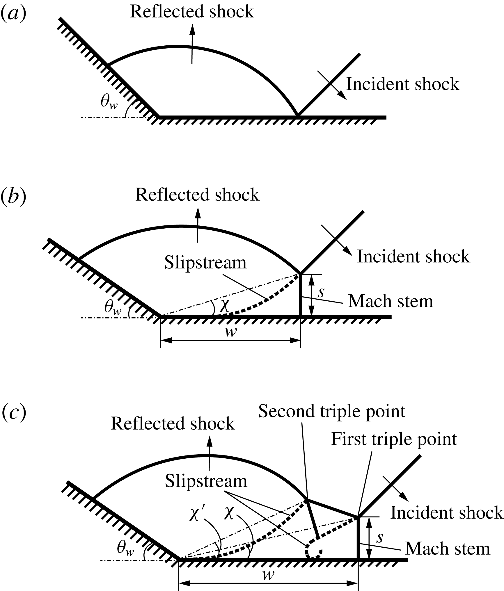
. Figure 1 shows two types of reflection patterns, regular and irregular reflections, where two kinds of irregular reflections, single-Mach reflection and double-Mach reflection, are presented (Ben-Dor & Takayama Reference Ben-Dor and Takayama1992; Ben-Dor Reference Ben-Dor2007). In figure 1,
 $w$
and
 $s$
denote the horizontal and vertical displacements of the triple points,
 $\unicode[STIX]{x1D712}$
denotes the first triple point trajectory angle and
 $\unicode[STIX]{x1D712}^{\prime }$
denotes the second triple point trajectory angle.
Illustration of two types of shock wave reflection off solid wedges, regular and irregular reflections, where two kinds of irregular reflections are shown. (a) Regular reflection; (b) irregular reflection: single-Mach reflection; (c) irregular reflection: double-Mach reflection.

Shock reflection patterns can be analysed in terms of the transition status and the reflection configuration. The transition status can be quantified using the transition angle, which determines when the reflection configuration transforms from irregular to regular. The reflection configuration can be described using the triple point trajectories. Using numerical methods, a high level of resolution can nowadays be achieved and can facilitate analysis of transition status and reflection configuration. Further, in shock wave experiments, the maximally achievable Mach number regimes can be limited due to the experimental set-up, while in simulations, such limitation does not exist. Thus, numerical simulations provide a practical approach to investigate shock wave reflection phenomena.
Various experimental visualization techniques have been performed in shock tube set-ups to determine the transition angle using either high temporal imaging or spatial imaging (Geva, Ram & Sadot Reference Geva, Ram and Sadot1990; Mouton Reference Mouton2006; Skews & Kleine Reference Skews and Kleine2010; Naidoo & Skews Reference Naidoo and Skews2011; Skews & Blitterswijk Reference Skews and Blitterswijk2011; Kleine et al. Reference Kleine, Timofeev, Hakkaki-Fard and Sadot2014; Ram, Geva & Sadot Reference Ram, Geva and Sadot2015). Technological advances of high temporal imaging equipment have made these systems readily available to many researchers. However, photographs from high-speed cameras often result in relatively low resolution due to high frame rates. Therefore, high temporal imaging can be used to understand succinct details of the entire process, but high spatial imaging will ultimately be required to provide accurate information (Versluis Reference Versluis2013). Nevertheless, studies to determine the transition angle using a combination of both high temporal and high spatial imaging are still lacking. Accordingly, in the current study, schlieren visualization with both high spatial and high temporal resolution are used to find the transition angles.
1.1 Shock reflection off a solid wedge
Although much attention has been given to establishing a transition criterion from regular to irregular reflections, work is still ongoing because of unsatisfactory comparison between numerical and experimental findings with theoretical solutions. Theoretical solutions are based on inviscid Euler analysis, while in experiments researchers must deal with viscosity and surface roughness of the reflecting surface. One widely used transition criterion for regular to irregular reflection is the detachment criterion, originally proposed by von Neumann (Reference von Neumann1943a ,Reference von Neumann b ). The detachment criterion (von Neumann Reference von Neumann1943a ) is an analytic solution of the transition angle for shock reflection off solid wedges in inviscid flow. The detachment criterion predicts that transition from regular to irregular reflection occurs when the maximum flow deflection angle across the reflected shock is achieved and the regular reflection is no longer possible. The detachment criterion states that in steady flow, the flow velocities ahead of the incident shock and behind the reflected shock remain parallel while the flow deflection by the reflected shock wave is maximal.
In shock wave reflection configurations of pseudo-steady cases, the appearance of Mach stems and slipstreams can be an important feature to distinguish between regular and irregular reflection. Usually, at small wedge angles, the reflection configurations remain irregular, where Mach stems and slipstreams are clearly seen. While approaching the transition condition by, for example, increasing the inclination angle of the wedge, the length of the Mach stem decreases as the triple point moves closer to the reflecting surface. As the inclination angle is increased to a certain angle, the reflection configuration transitions from irregular to regular reflection. The critical
 $\unicode[STIX]{x1D703}_{w}$
at the transition status between irregular to regular reflection is referred to as the transition angle.
Shock wave reflection over solid wedges has been investigated previously by numerous research groups (Mach Reference Mach1878; von Neumann Reference von Neumann1943a
,Reference von Neumann
b
; Hornung, Oertel & Sandeman Reference Hornung, Oertel and Sandeman1979; Hornung & Robinson Reference Hornung and Robinson1982; Hornung & Taylor Reference Hornung and Taylor1982; Ben-Dor et al.
Reference Ben-Dor, Mazor, Takayama and Igra1987; Onodera & Takayama Reference Onodera and Takayama1990; Sasoh, Takayama & Saito Reference Sasoh, Takayama and Saito1992; Skews Reference Skews2005). Hornung & Taylor (Reference Hornung and Taylor1982) experimentally explored the influence of viscosity on the transition from regular to Mach reflection of strong shock waves (
 $M_{s}=5.5$
). Argon was used to avoid real gas effects, and results showed that in pseudo-steady flows viscosity plays an important role such that the transition angle was affected by up to
 $7^{\circ }$
compared to the case with no viscosity.
One major difference between a solid and a water wedge is that, compared to solid wedges, the surface of a water wedge can be treated as perfectly smooth. However, the surface roughness for a solid wedge may be hard to quantify due to uncertainties in measurements. To quantify the effect of surface roughness, Ben-Dor et al. (Reference Ben-Dor, Mazor, Takayama and Igra1987) proposed a boundary-layer displacement thickness model for predicting regular to Mach reflection transition. The model is specified for incident shock Mach numbers in the range of
 $1<M_{s}<2$
, and surface roughness heights up to 2 mm. Results showed that the flow behind the reflection point must be parallel to the average slope of the displaced surface. Onodera & Takayama (Reference Onodera and Takayama1990) used both numerical and experimental methods to study the effect of slit wedges on shock wave transition. Incident Mach numbers ranged from 1.07 to 3.03, and slit wedges with perforation ratios 0.34 and 0.4 were used. Perforation ratio is defined as the ratio of the perforated and overall surface area. Results showed that for stronger shock waves and a perforation ratio of 0.4, the transition angle was decreased by approximately
 $10^{\circ }$
as compared with the detachment criterion. The numerical results agreed well with experimental results. More recently, Skews (Reference Skews2005) experimentally extended this study to a wider range of plate geometries. It was found that the plate thickness had a negligible influence on the results for the tested parameter range.
Shock wave reflection off curved surfaces have also been an area of interest. Kleine et al. (Reference Kleine, Timofeev, Hakkaki-Fard and Sadot2014) experimentally and numerically investigated the influence of the Reynolds number on the triple point trajectories where a planar shock wave is reflected by cylindrical surfaces. Results showed that the delay of the transition between regular reflection (RR) and Mach reflection (MR) due to viscous effects is low under high Reynolds numbers. More recently, Soni et al. (Reference Soni, Hadjadj, Chaudhuri and Ben-Dor2017) performed numerical simulations to study the wave configurations related to the shock reflection over double-concave cylindrical surfaces. The study covered different incident shock Mach numbers as well as geometrical parameters of the reflectors, such as the radii of curvature and the initial wedge angles. Noticeable differences can be found between the shock patterns over the two adjacent reflectors of the same shape, where the shock reflection off the second reflector is strongly dependent on how fast the diffracted shock reaches the incident shock wave.
1.2 Triple point trajectories
The reflection configurations of single-Mach reflection and double-Mach reflection can be quantified by tracking the triple point trajectories. For single-Mach reflection, based on the assumptions that the shock wave configuration is self-similar and the triple point trajectories are straight lines emanating from the compressive corner, an analytic formulation (Law Reference Law1970; Ben-Dor Reference Ben-Dor1978; Ben-Dor & Glass Reference Ben-Dor and Glass1979, Reference Ben-Dor and Glass1980) was developed to describe the motion of the triple point trajectory angle, which is illustrated by
 $\unicode[STIX]{x1D712}$
in figure 1(b). Assumptions include a straight Mach stem normal to the wedge surface and uniform inviscid flow behind incident shock wave, reflected shock wave and Mach stem. The method to solve for the triple point trajectory angle in single-Mach reflection also applies for the first triple point in the case of a double-Mach reflection,
 $\unicode[STIX]{x1D712}$
in figure 1(c).
For the second triple point trajectory angle, denoted
 $\unicode[STIX]{x1D712}^{\prime }$
in figure 1(c), Ben-Dor (Reference Ben-Dor1980, Reference Ben-Dor1981) formulated an analytic solution to describe the relative motion of the second triple point in terms of the first triple point. They also concluded that the triple point trajectory angle of the second triple point should be always greater than the first one. Later, Li & Ben-Dor (Reference Li and Ben-Dor1995) proposed a new analytic model to predict the second triple point trajectory of a double-Mach reflection. The new model improved the prediction tremendously by replacing the Law–Glass assumption by models accounting for the interaction of the shock wave reflection and the shock induced flow deflection processes.
1.3 Shock interaction with liquid
Both experiments and numerical simulations of a planar shock wave interaction with a liquid droplet have been performed by Igra & Takayama (Reference Igra and Takayama2001a
,Reference Igra and Takayama
b
). They proposed a numerical scheme to achieve a sharp interface between the gas and liquid phase. Tait’s equation of state was employed for water with
 $n=7.415$
and
 $B=296.3$
MPa. With that scheme, shock wave interaction with a cylindrical water column was modelled and good agreement was shown compared with experimental interferogram results. More recently, Meng & Colonius (Reference Meng and Colonius2015) have numerically modelled the early stage of the breakup of water cylinders in the flow behind normal shock waves. The simulations were performed in a two-dimensional domain with symmetric boundary conditions, where the stiffened gas equation of state was used to model both gases and liquids. Numerical schlieren images were compared with previous experimental findings (Igra & Takayama Reference Igra and Takayama2001a
), and agreement was shown regarding the breakup process of the cylinders. In particular, the water cylinder was first compressed in the streamwise direction and then extended in its spanwise dimension.
Planar shock wave reflection over water wedges has been experimentally studied by Takayama & Ben-Dor (Reference Takayama and Ben-Dor1989). In their study, experiments were conducted using an inclined shock tube that could be tilted from a horizontal to a vertical direction with an accuracy of
 $0.1^{\circ }$
. Four different types of reflection configurations were observed: regular reflection, single-Mach reflection, transitional-Mach reflection and double-Mach reflection. Measurements of the transition angles showed good agreement with the detachment criterion for the incident shock wave Mach number in the range
 $M_{s}>1.47$
, and poor agreement for
 $M_{s}<1.47$
. The theory of irregular reflection from von Neumann (Reference von Neumann1943a
), also called three-shock theory, showed good agreement for strong shocks, i.e.
 $M_{s}>1.47$
(Colella & Henderson Reference Colella and Henderson1990), but for weak shocks, the three-shock theory showed that the Mach reflection is physically impossible for
 $M_{s}<1.035$
. The discrepancy between the three-shock theory and experimental results was referred to as the von Neumann paradox (Birkhoff Reference Birkhoff1950). Colella & Henderson (Reference Colella and Henderson1990) experimentally and numerically showed that Mach reflection was still possible for weak shocks. It was later confirmed later by Baskar, Coulouvrat & Marchiano (Reference Baskar, Coulouvrat and Marchiano2007), Marchiano et al. (Reference Marchiano, Coulouvrat, Baskar and Thomas2007), Karzova et al. (Reference Karzova, Khokhlova, Salze, Ollivier and Blanc-Benon2015) and Desjouy et al. (Reference Desjouy, Ollivier, Marsden, Karzova and Blanc-Benon2016) that irregular reflection and establishment of Mach stem could occur even for very weak shocks, i.e.
 $1.0001<M_{s}<1.01$
. Additionally, one likely reason for the poor agreement was that the detachment criterion assumed uniform flow states behind reflected shock wave and Mach stem, while this assumption was incorrect when subsonic flow regions were involved. However, apart from the study of Takayama & Ben-Dor (Reference Takayama and Ben-Dor1989), shock reflections over liquid surfaces remain largely unexplored. This may be the result of challenges associated with performing experiments on liquid boundaries, and performing numerical simulations featuring multiphase phenomena with a deforming free surface. To investigate shock wave reflections at an air–water interface, previous research analytically calculated the energy exchange during shock reflection off an air–water interface, and results showed that nearly all of the incident energy is reflected back due to the impedance mismatch between the air and water (Sakurai Reference Sakurai1974; Henderson et al.
Reference Henderson, Ma, Sakurai and Takayama1990). Borisov, Kogarko & Lyubimov (Reference Borisov, Kogarko and Lyubimov1965) first proposed the existence of shock wave refraction when a shock wave is sliding over a water layer, and meanwhile a precursor shock is formed in the air. Later, the refraction phenomenon was confirmed experimentally by Teodorczyk & Shepherd (Reference Teodorczyk and Shepherd2012). More recently, Rodriguez et al. (Reference Rodriguez, Jourdan, Marty, Allou and Parisse2016) experimentally studied shock waves sliding over a horizontal free water layer. Two incident shock Mach numbers,
 $M_{s}=1.11$
and 1.43, were examined and the incident shock wave was vertical compared to the water surface. Results show that the transmitted shock wave in the water is ahead of the shock wave in the air. Further, the observed compression wave in the water travels at the same speed as the shock wave in the air, which is slower than the speed of sound in water. Thus, the propagation of the compression wave is driven by the shock wave in the air.
1.4 Equation of state
To numerically model water, two kinds of equations of state are typically used; (i) Tait’s equation of state and (ii) a stiffened gas equation of state. Tait’s equation of state, which is designed to describe the compressibility of water, has the form
 $$\begin{eqnarray}\frac{p+B(s)}{p_{0}+B(s)}=\left(\frac{\unicode[STIX]{x1D70C}}{\unicode[STIX]{x1D70C}_{0}}\right)^{n},\end{eqnarray}$$
where subscript 0 refers to ambient conditions,
 $s$
denotes entropy,
 $p$
pressure and
 $\unicode[STIX]{x1D70C}$
density. Some researchers state that
 $B(s)$
and
 $n$
can be treated as constants for pressures up to
 $10^{4}$
MPa (Kedrinskii Reference Kedrinskii2005). Therefore,
 $B$
and
 $n$
are chosen such that density,
 $\unicode[STIX]{x1D70C}_{0}$
, and speed of sound,
 $a_{0}$
, are properly estimated through
 $$\begin{eqnarray}B=\unicode[STIX]{x1D70C}_{0}{a_{0}}^{2}/n,\quad a_{0}=\sqrt{\frac{\unicode[STIX]{x1D6FE}(p_{\infty }+p)}{\unicode[STIX]{x1D70C}}}.\end{eqnarray}$$
The following numerical values are most commonly used in the Tait’s equation of state,
 $B=296.3$
, 304.7 and 321.4 MPa, and
 $n=7.415$
, 7.15 and 7 (Cole Reference Cole1948; Ridah Reference Ridah1988; Igra & Takayama Reference Igra and Takayama2001a
,Reference Igra and Takayama
b
). A detailed examination of equations and charts for shock waves in water has been produced by Ridah (Reference Ridah1988), who used
 $n=7$
and
 $B=321.4$
MPa resulting in
 $a_{0}=1500~\text{m}~\text{s}^{-1}$
.
The stiffened gas equation of state takes the form
 $$\begin{eqnarray}p=(\unicode[STIX]{x1D6FE}-1)\unicode[STIX]{x1D70C}e-\unicode[STIX]{x1D6FE}p_{\infty },\end{eqnarray}$$
where
 $e$
is the specific total energy and
 $\unicode[STIX]{x1D6FE}$
and
 $p_{\infty }$
are two empirically determined constants. When
 $p_{\infty }=0$
, the stiffened gas equation of state reverts to the perfect gas equation of state. Assuming a constant specific heat at constant volume,
 $c_{v}$
, the internal energy in the stiffened gas model reads (Flåtten, Morin & Munkefjord Reference Flåtten, Morin and Munkefjord2011)
 $$\begin{eqnarray}e=c_{v}T+\frac{p_{\infty }}{\unicode[STIX]{x1D70C}},\end{eqnarray}$$
which allows expressing (1.3) in terms of the temperature as
 $$\begin{eqnarray}p+p_{\infty }=(\unicode[STIX]{x1D6FE}-1)\unicode[STIX]{x1D70C}c_{v}T.\end{eqnarray}$$
The two constants are most often set to
 $p_{\infty }=600$
and 300 MPa,
 $\unicode[STIX]{x1D6FE}=4.4$
, 5.5 and 7.0 (Grove & Menikoff Reference Grove and Menikoff1990; Saurel & Abqrall Reference Saurel and Abgrall1999; Shyue Reference Shyue1999). Jolgam et al. (Reference Jolgam, Ballil, Nowakowski and Nicolleau2012) used a few test problems to verify the performance of a proposed Eulerian numerical method simulating multiphase flows, air and water, while simultaneously comparing the computational cost of different equations of state. Both stiffened gas and van der Waals equation of state were used for air, while stiffened gas and Tait’s equation of state were utilized for water. Three test problems consisting of a water–air shock tube, a gas–air shock tube and a water faucet test, were considered. Results showed that the van der Waals equation of state needed more time steps and central processing unit (CPU) time than the stiffened gas equation of state to obtain the solution, while stiffened gas (with
 $\unicode[STIX]{x1D6FE}=4.4$
and
 $p_{\infty }=600$
MPa) and Tait’s equation of state (with
 $n=7.15$
and
 $B=331$
MPa) for water needed approximately the same number of time steps and the same CPU time. Moreover, in their study, the stiffened gas equation of state for water was defined using constants
 $\unicode[STIX]{x1D6FE}=4.4$
and
 $p_{\infty }=600$
MPa, while Tait’s equation of state was defined with
 $n=7.15$
and
 $B=331$
MPa.
In this study, an inviscid shock-capturing multiphase solver is used to simulate shock wave behaviour at air–water interfaces in a two-dimensional domain. Six different incident shock Mach numbers,
 $M_{s}=1.2$
, 1.38, 1.52, 2, 3 and 4, are used in the simulations and three different shock Mach numbers,
 $M_{s}=1.20$
, 1.38 and 1.52, are investigated in the experiments. Shock reflection solutions from water wedges are compared with those from solid wedges. In particular, transition angles from regular to irregular reflection for both water and solid wedges were obtained for a range of incident shock Mach numbers. Further, in order to quantify the reflection configuration, the trajectories of triple points in both single-Mach reflection and double-Mach reflection were measured. Finally, the results from the numerical simulations were compared to experimental data using schlieren visualization.
2 Numerical approach
A two-dimensional flow field was considered, where for both solid and water wedge cases the wedge surface was impacted by a planar shock wave.
2.1 Governing equations
The set of used governing equations is based on a multicomponent model that employs the phase volume fractions
 $\unicode[STIX]{x1D6FC}^{i}$
with
 $\sum _{i=1}^{m}\unicode[STIX]{x1D6FC}^{i}=1$
. Mixture quantities are given as
 $$\begin{eqnarray}\unicode[STIX]{x1D70C}=\mathop{\sum }_{i=1}^{m}\unicode[STIX]{x1D6FC}^{i}\unicode[STIX]{x1D70C}^{i},\quad \unicode[STIX]{x1D70C}\boldsymbol{u}=\mathop{\sum }_{i=1}^{m}\unicode[STIX]{x1D6FC}^{i}\unicode[STIX]{x1D70C}^{i}\boldsymbol{u}^{i},\quad \unicode[STIX]{x1D70C}e=\mathop{\sum }_{i=1}^{m}\unicode[STIX]{x1D6FC}^{i}\unicode[STIX]{x1D70C}^{i}e^{i}.\end{eqnarray}$$
In this description, multiple fluids are represented as mostly separated phases that can be described by a single set of two-dimensional inviscid Euler equations
 $$\begin{eqnarray}\displaystyle & \unicode[STIX]{x2202}_{t}\unicode[STIX]{x1D70C}+\unicode[STIX]{x1D735}\boldsymbol{\cdot }(\unicode[STIX]{x1D70C}\boldsymbol{u})=0, & \displaystyle\end{eqnarray}$$
 $$\begin{eqnarray}\displaystyle & \unicode[STIX]{x2202}_{t}(\unicode[STIX]{x1D70C}\boldsymbol{u})+\unicode[STIX]{x1D735}\boldsymbol{\cdot }(\unicode[STIX]{x1D70C}\boldsymbol{u}\otimes \boldsymbol{u})+\unicode[STIX]{x1D735}p=0, & \displaystyle\end{eqnarray}$$
 $$\begin{eqnarray}\displaystyle & \unicode[STIX]{x2202}_{t}(\unicode[STIX]{x1D70C}E)+\unicode[STIX]{x1D735}\boldsymbol{\cdot }((\unicode[STIX]{x1D70C}E+p)\boldsymbol{u})=0, & \displaystyle\end{eqnarray}$$
which represent the conservation of mixture mass, mixture moment and total energy without any body forces. Here,
 $\boldsymbol{u}$
is the velocity vector and
 $E=e+(1/2)\boldsymbol{u}^{\text{T}}\boldsymbol{u}$
the specific total energy. Applying a stiffened gas equation of state
 $$\begin{eqnarray}p^{i}=(\unicode[STIX]{x1D6FE}^{i}-1)\unicode[STIX]{x1D70C}^{i}e^{i}-\unicode[STIX]{x1D6FE}^{i}p_{\infty }^{i}=(\unicode[STIX]{x1D6FE}^{i}-1)\unicode[STIX]{x1D70C}^{i}c_{v}^{i}T^{i}-p_{\infty }^{i},\end{eqnarray}$$
the total hydrodynamic pressure
 $p$
and
 $p_{\infty }$
of the mixture are given as
 $$\begin{eqnarray}\frac{p}{\unicode[STIX]{x1D6FE}-1}=\mathop{\sum }_{i=1}^{m}\frac{\unicode[STIX]{x1D6FC}^{i}p^{i}}{\unicode[STIX]{x1D6FE}^{i}-1},\quad \frac{\unicode[STIX]{x1D6FE}p_{\infty }}{\unicode[STIX]{x1D6FE}-1}=\mathop{\sum }_{i=1}^{m}\frac{\unicode[STIX]{x1D6FC}^{i}\unicode[STIX]{x1D6FE}^{i}p_{\infty }^{i}}{\unicode[STIX]{x1D6FE}^{i}-1}.\end{eqnarray}$$
Instead of using propagation equations of
 $\unicode[STIX]{x1D6FC}^{i}$
to distinguish the components, the approach of Shyue (Reference Shyue1998) has been adopted to supplement equations (2.2)–(2.4) with the two advection equations
 $$\begin{eqnarray}\displaystyle & \displaystyle \frac{\unicode[STIX]{x2202}}{\unicode[STIX]{x2202}t}\left(\frac{1}{\unicode[STIX]{x1D6FE}-1}\right)+\boldsymbol{u}\boldsymbol{\cdot }\unicode[STIX]{x1D735}\left(\frac{1}{\unicode[STIX]{x1D6FE}-1}\right)=0, & \displaystyle\end{eqnarray}$$
 $$\begin{eqnarray}\displaystyle & \displaystyle \frac{\unicode[STIX]{x2202}}{\unicode[STIX]{x2202}t}\left(\frac{\unicode[STIX]{x1D6FE}p_{\infty }}{\unicode[STIX]{x1D6FE}-1}\right)+\boldsymbol{u}\boldsymbol{\cdot }\unicode[STIX]{x1D735}\left(\frac{\unicode[STIX]{x1D6FE}p_{\infty }}{\unicode[STIX]{x1D6FE}-1}\right)=0. & \displaystyle\end{eqnarray}$$
Although this description is applicable only to two-component systems, i.e.
 $m=2$
, the benefit is that the direct utilization of (2.7), (2.8) in the governing equations and therefore direct discretization together with (2.2)–(2.4) is the simplest remedy (Shyue Reference Shyue2006) to the otherwise intrinsic problem of non-physical numerical pressure oscillations at interfaces with vastly different parameters
 $\unicode[STIX]{x1D6FE}^{i}$
and
 $p_{\infty }^{i}$
(Abgrall & Karni Reference Abgrall and Karni2001). Here, the parameters for water were defined as
 $\unicode[STIX]{x1D6FE}^{W}=7.0$
and
 $p_{\infty }^{W}=300$
MPa (Grove & Menikoff Reference Grove and Menikoff1990; Shyue Reference Shyue1999), resulting in an ambient speed of sound of
 $a_{0}=1452~\text{m}~\text{s}^{-1}$
and
 $\unicode[STIX]{x1D6FE}^{A}=1.4$
and
 $p_{\infty }^{A}=0$
for air.
2.2 Numerical method
A time-explicit finite volume approach is used to discretize the governing equations with the second-order accurate wave propagation method (LeVeque Reference LeVeque2002). This method is designed for schemes in flux-difference splitting form and can handle the conservative equations (2.2)–(2.4) with an approximate Riemann solver as well as the non-conservative advection equations (2.7) and (2.8). In order to cope with realistic density differences across the air–water interface, the Harten–Lax–van Leer with contact (HLLC) scheme by Toro, Spruce & Speares (Reference Toro, Spruce and Speares1994) is used as approximate Riemann solver. An extended version of the HLLC scheme, tailored for the above set of governing equations for two-phase flow and smoothly incorporated into the wave propagation approach had been specially derived (Deiterding, Cirak & Mauch Reference Deiterding, Cirak, Mauch, Hartmann, Meister, Schäfer and Turek2009). Thanks to the robustness of the HLLC approach, the subsequent computations could use the accurate densities
 $\unicode[STIX]{x1D70C}^{W}=997~\text{kg}~\text{m}^{-3}$
and
 $\unicode[STIX]{x1D70C}^{A}=1.18~\text{kg}~\text{m}^{-3}$
.
In order to enable technically relevant computations, the sketched finite volume method has been incorporated into the Cartesian adaptive mesh refinement solver system AMROC V2.0 (Deiterding Reference Deiterding2011) within the freely available fluid–structure coupling software Virtual Test Facility (Deiterding et al. Reference Deiterding, Radovitzky, Mauch, Noels, Cummings and Meiron2006). The consideration of geometrically complex boundaries in AMROC is achieved by a generic and discretization-independent level set technique. Based on signed distance information stored in the level set function, reflective wall boundary conditions are constructed by inter- and extrapolation operations in cells adjacent to the boundary, but deemed outside of the fluid domain, before the Cartesian discretization is employed to compute the next time step (Deiterding Reference Deiterding2009). Block-based mesh refinement is applied and regenerated consecutively at run time to mitigate inaccuracies from the boundary approximation as well as to capture essential flow features, like shock waves and material interfaces with increased resolution (Deiterding Reference Deiterding2011). Time step refinement by the same factor as the spatial refinement ensures that the stability condition of the explicit finite volume scheme is in principle satisfied on all refinement levels.
Validation simulations for the sketched dynamically adaptive two-phase HLLC method are provided by Perotti et al. (Reference Perotti, Deiterding, Inaba, Shepherd and Ortiz2013), where elastic deformations of tubes from shock waves in water have been analysed meticulously. Further verification and validation simulations for water hammer and underwater explosion driven plastic deformation and rupture of metallic plates with two-phase flow and empirical cavitation modelling are given by Cirak, Deiterding & Mauch (Reference Cirak, Deiterding and Mauch2007) and Deiterding et al. (Reference Deiterding, Cirak, Mauch, Hartmann, Meister, Schäfer and Turek2009).
2.3 Simulation set-up
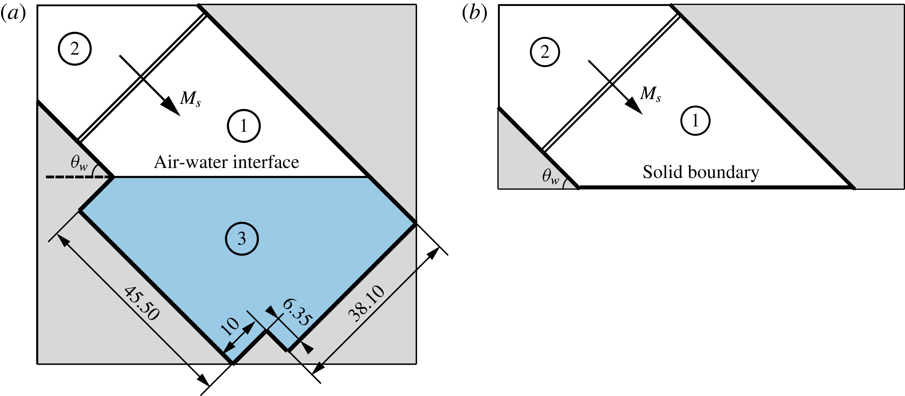
The simulation time for each case is chosen such that the incident shock wave has enough time to impact the air–water interface and reach the corner formed by the wedge and the outer solid boundary and reflect back. During this time period, the displacement of fluid particles due to gravity is negligible. The geometrical set-up for the water and solid wedge cases is shown in figures 2(a) and 2(b), respectively. The rectangular outer frames represent the boundaries of the computational domains, while the oblique thick lines denote the boundary of the test section. In figure 2(a), the shape of the geometrical set-up is chosen to match an experimental set-up to enable comparison of experimental and numerical results. Results from shock reflection off a liquid wedge were compared to those off a solid wedge. The inclination angle of the wedge is denoted
 $\unicode[STIX]{x1D703}_{w}$
, see figure 2(a,b). The boundary condition of the upper left corner of the computational domain was set-up as a constant inlet flow while the rest of the boundaries were modelled as rigid walls.
Set-up for numerical simulations of shock wave reflection off (a) a water wedge and (b) a solid wedge. Regions 1 and 2 and are filled with air while region 3 is filled with water. Dimensions in mm, not to scale.

Cartesian grids were applied to the whole computational domain. For all the simulations, adaptive mesh refinement (AMR) was applied during the simulation. The dynamic mesh refinement was based on the scaled gradients of pressure, density and volume fraction
 $\unicode[STIX]{x1D6FC}_{i}$
as well as of the level set representing the rigid boundaries. Three AMR levels were chosen and a refinement factor of 2 was used. A coarse background grid of cell size
 $100\times 100~\unicode[STIX]{x03BC}\text{m}^{2}$
was created so after mesh refinement, the smallest effective cell size was
 $25\times 25~\unicode[STIX]{x03BC}\text{m}^{2}$
.
Initial conditions ahead of the incident shock wave, denoted region 1 in both figures 2(a) and 2(b), were set-up with standard atmospheric conditions:
 $p_{1}=1.013\times 10^{5}$
Pa,
 $\unicode[STIX]{x1D70C}_{1}=1.18~\text{kg}~\text{m}^{-3}$
and
 $T_{1}=25\,^{\circ }\text{C}$
. The conditions behind the incident shock wave, region 2 in figure 2, were determined using normal shock relations. Region 3 shown in figure 2(a) was filled with water at atmospheric pressure and room temperature, same as region 1. The resulting density of water is
 $\unicode[STIX]{x1D70C}_{3}=997~\text{kg}~\text{m}^{-3}$
. All the simulations assumed inviscid flow and the solid wedge surface to be rigid and smooth.
Each simulation of a shock reflecting off a water wedge took approximately 25 CPU hours using a single core of 3.20 GHz Intel(R) Core(TM) i7-3930K CPU, but only 11 CPU hours for shock reflection off a solid wedge.
The transition angle measured through the simulations fell into a range with uncertainty of
 $1^{\circ }$
because the inclination wedge angle was increased by increments of
 $1^{\circ }$
after each run.
2.4 Constraints of the numerical simulation
Without the presence of viscosity, the shock reflection patterns are affected in two ways. (i) For irregular shock reflection, viscosity delays the establishment of the Mach stem. Kleine et al. (Reference Kleine, Timofeev, Hakkaki-Fard and Sadot2014) confirmed that the Reynolds number mainly affects the initial establishment of the Mach stem and only to a lesser degree its subsequent growth. Thus, in terms of shock patterns, the Mach stem is established earlier without viscosity, but the triple point trajectory angle is not much affected. (ii) Viscosity decreases the transition angle, and therefore simulation results in this study are compared with experiments, shock reflection over the solid wedge cases and the analytical solution under the same inviscid assumption.
The entire computational domain was meshed using a Cartesian grid. Because of the nature of the Cartesian grid, when a shock wave, air–water interface or physical boundary is not aligned with the grid, assignment of the initial conditions to the corresponding cells results in a sawtooth-shaped discontinuity or boundary, which leads to an addition of artificial roughness. Although the artificial roughness can be reduced by refining the grid size, it is never eliminated as long as the Cartesian mesh is used. The same grid effect can be found in the work of Soni et al. (Reference Soni, Hadjadj, Chaudhuri and Ben-Dor2017). The artificial roughness may delay the establishment of the Mach stem and therefore affect transition angles. Thus, a convergence test using six different mesh sizes, i.e.
 $200~\unicode[STIX]{x03BC}\text{m}$
,
 $100~\unicode[STIX]{x03BC}\text{m}$
,
 $50~\unicode[STIX]{x03BC}\text{m}$
,
 $30~\unicode[STIX]{x03BC}\text{m}$
,
 $25~\unicode[STIX]{x03BC}\text{m}$
and
 $15~\unicode[STIX]{x03BC}\text{m}$
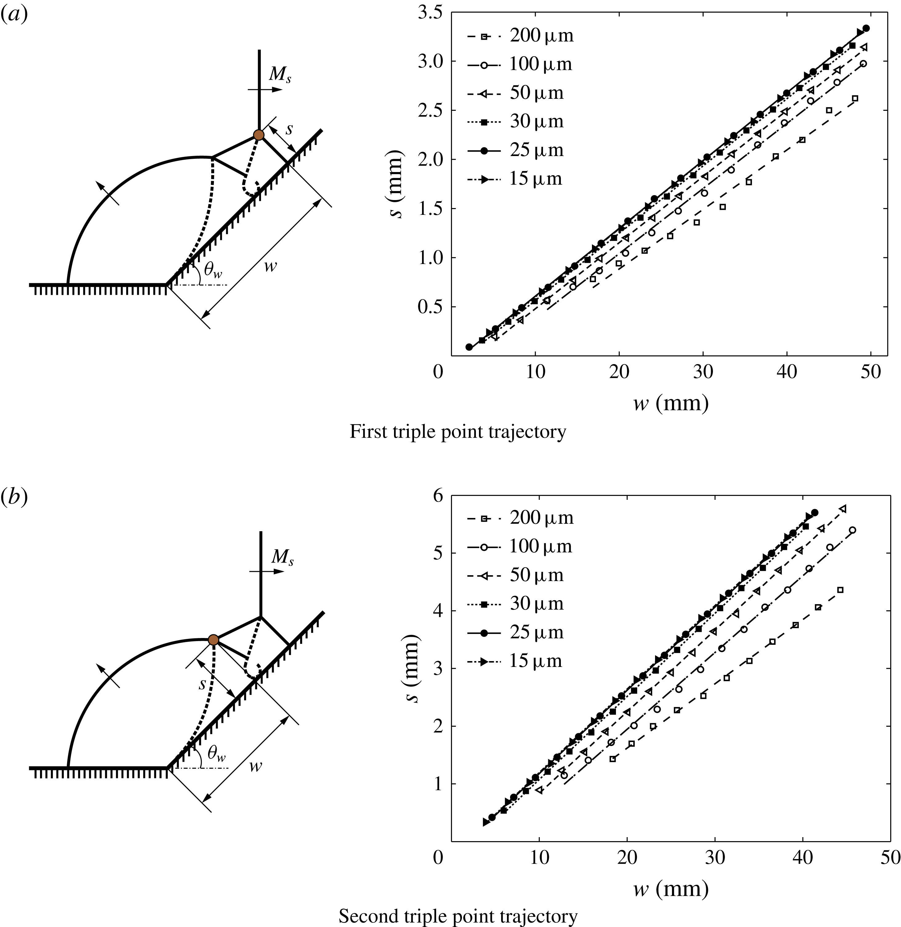
, with regard to the triple point trajectories is conducted for the solid wedge case with
 $M_{s}=3$
and
 $\unicode[STIX]{x1D703}_{w}=45^{\circ }$
, as shown in figure 3. The convergence study is used to prove that results of triple point trajectories are independent of grid size and the mesh is refined enough. In the convergence study, the angle formed between the wedge surface and the Cartesian grid is
 $45^{\circ }$
. Results obtained from grid sizes
 $25~\unicode[STIX]{x03BC}\text{m}$
and
 $15~\unicode[STIX]{x03BC}\text{m}$
show negligible difference. Therefore, the grid size,
 $25~\unicode[STIX]{x03BC}\text{m}$
, is determined to be refined enough to capture the initiation of the Mach stem and this grid size is used in all the other shock wave reflection simulations.
Mach stem heights
 $s$
versus displacement in the horizontal direction
 $w$
for the (a) first triple point and (b) second triple point at
 $M_{s}=3$
and
 $\unicode[STIX]{x1D703}_{w}=45^{\circ }$
solid wedge. Results obtained with different grid sizes.

The liquid surface tension is not considered in the simulations. However, the lack of surface tension does not affect the shock reflection patterns and corresponding results, since the deformation of the interface is negligible during the simulated time.
Due to the nature of the shock-capturing scheme, shock waves and interfaces are diffusive and spread over several grid cells. Therefore, the mixture regions near the air–water interface do not indicate the molecular mixing of the two-phase flow, but are because of the non-physical numerical diffusion.
3 Experimental approach
Experiments are performed using an adjustable, inclined shock tube and schlieren visualization with either high spatial or high temporal resolution.
3.1 Details of the shock tube
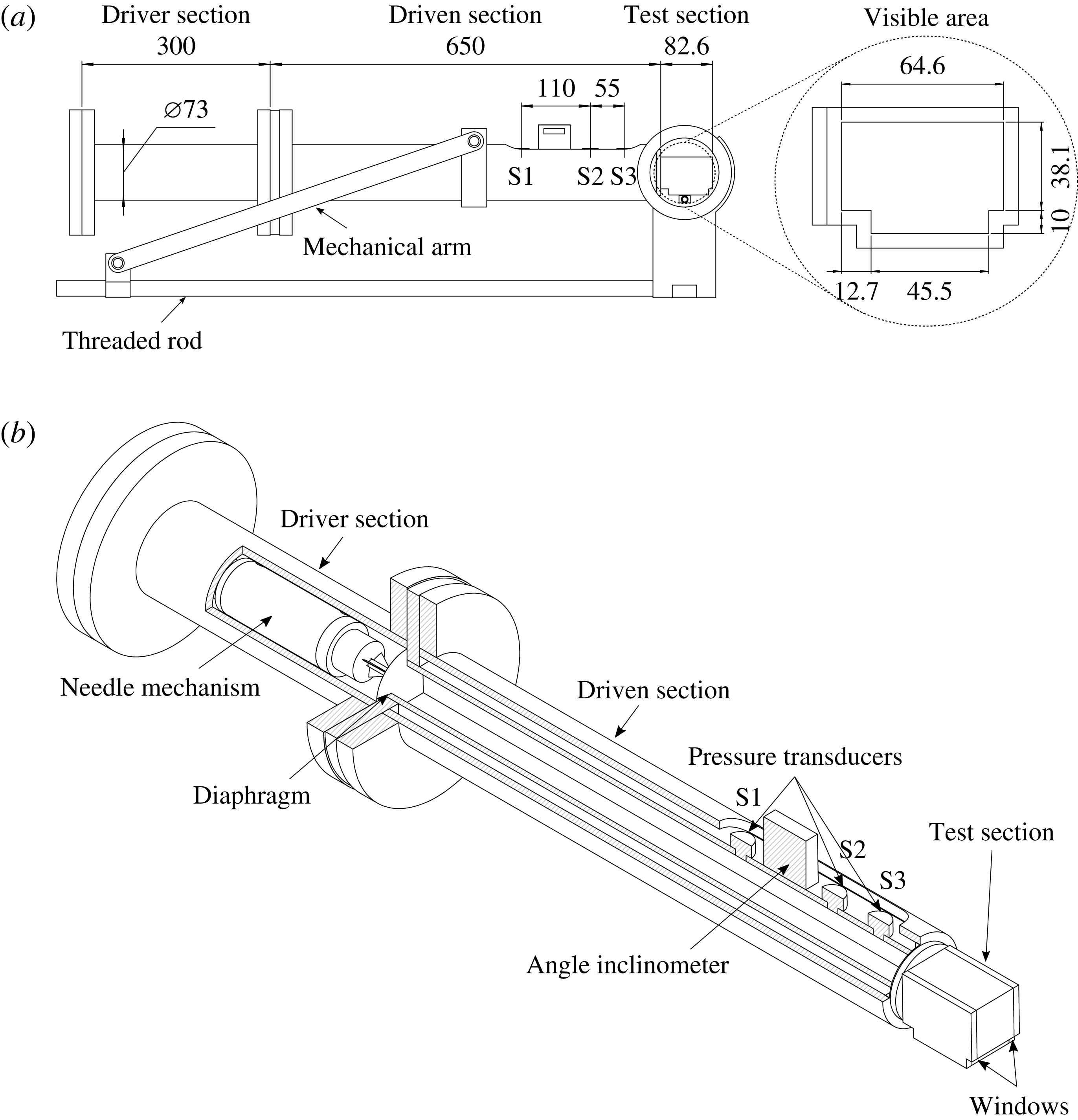
The experimental set-up uses an inclined shock tube for which the inclination angle can be adjusted, as shown in figure 4(a). The shock tube was designed to study shock wave reflection off solid and liquid wedges, and as such the inclination angle of the shock tube can be adjusted in the range
 $0^{\circ }<\unicode[STIX]{x1D703}_{w}<90^{\circ }$
. The angle of the shock tube is controlled by moving a support arm along an Acme threaded rod, which travels 6.4 mm per rotation and the angle is measured by an inclinometer (Wixey WR365,
 $\pm 0.1^{\circ }$
accuracy). The shock tube consists of a driver section, a driven section with square interior sides and a test section. The driver section of the inclined shock tube is 300 mm long and has a 73 mm diameter circular cross-section. The driven section and the test section both have square 38.1 mm inner sides. The length of the driven section is approximately 17 times longer than the side of the test section to ensure that the shock is planar upon arriving in the test section (Bleakney, Weimer & Fletcher Reference Bleakney, Weimer and Fletcher1949). A diaphragm is located between the driver and driven sections, and a shock wave can be generated after the diaphragm rupture by a needle mechanism in the driver section (Jeon et al.
Reference Jeon, Gross, Estabrook, Koumlis, Wan, Khanolkar, Tao, Mensching, Lesnick and Eliasson2015). Three different thicknesses of moisture-resistant polyester film (12.7, 25.4 and
 $50.8~\unicode[STIX]{x03BC}\text{m}$
thickness,
 $\pm$
10 % tolerance) were used as diaphragm materials to perform experiments featuring driver pressures of 138, 310 and 586 kPa (20, 45 and 85 psi), respectively. The test section was designed as a ‘T’ shape to minimize the meniscus between the water surface and the solid wall of the test section. The windows of the test section were made of 12.7 mm thick Plexiglas. In the test section, two different types of reflecting surfaces are considered: water and solid wedges. Tap water is used at room temperature (300 K). The solid wedges are made of polycarbonate (Makrolon®GP sheet) with 10 different angles (from
 $40^{\circ }$
to
 $50^{\circ }$
) and care is taken to ensure that the reflecting surface of the polycarbonate sheet has a surface roughness similar to glass.
Schematic description of inclined shock tube: (a) side and cross-view of the inclined shock tube. Dimensions in mm; (b) detailed cut view of the inclined shock tube.

All experiments were conducted with air as test gas at atmospheric pressure (101 kPa) and room temperature (300 K). The shock Mach number was measured using three pressure transducers (S1 and S3: PCB 113B21, S2: PCB 113B31) placed in the driven section ahead of the test section, as shown in figure 4(b). The incident shock Mach number was determined using the elapsed time between the shock passing the three pressure transducers. The shock Mach numbers were measured with a standard deviation within
 $\pm$
0.70 % and a measurement uncertainty less than
 $\pm$
0.80 % in each experiment. After the pressure signals were recorded by the oscilloscope, a low pass Fourier filter was used to remove all frequencies above 100 kHz for data recorded by S1 and S3, and 80 kHz for data recorded by S2. The cutoff frequency was chosen such that it is below the natural frequency of the pressure transducer, which is 500 kHz for S1 and S3 and 400 kHz for S2.
3.2 Visualization set-up
For this study, schlieren visualization with both high spatial and high temporal resolution is used to compensate the respective drawbacks of the two techniques. Both methods are set-up to avoid motion blur (Versluis Reference Versluis2013), which can be expressed as
 $$\begin{eqnarray}v\times \unicode[STIX]{x0394}t\leqslant \frac{P}{M_{im}},\end{eqnarray}$$
when
 $v$
is an object’s speed,
 $\unicode[STIX]{x0394}t$
is the exposure time of the camera or the light source,
 $P$
is the size of one pixel and
 $M_{im}$
is the image magnification factor. These two methods are summarized in table 1 and explained in detail in the following two subsections. To obtain quantitative data from the images, optical distortions resulting from the visualization system are corrected using the control point tool box in MATLAB (Delpino Gonzales & Eliasson Reference Delpino Gonzales and Eliasson2015).
Summary of camera settings.

Typically, the thickness of the shock wave is of the order of the mean free path of the gas, which at standard atmospheric conditions results in 200 nm shock thickness (Fox, McDonald & Pritchard Reference Fox, McDonald and Pritchard1985). In practice, the thickness of the dark band representing the shock wave that is obtained by using schlieren photography can be affected by several factors such as the strength of the shock wave, a non-parallel incident light angle and shadowgraph effects. In this experiment, when using the Phantom V711 camera, the thickness of the dark band was approximately equal to 1 pixel (
 $450~\unicode[STIX]{x03BC}\text{m}$
). However, when using the Nikon D90, it was approximately 10 pixels (
 $270~\unicode[STIX]{x03BC}\text{m}$
), similar to previous results (Ram et al.
Reference Ram, Geva and Sadot2015).
3.2.1 Schlieren visualization with high temporal resolution
High temporal resolution was obtained using a z-folded schlieren set-up (Wang & Eliasson Reference Wang and Eliasson2012) with a high-speed camera (Phantom V711) and a high-power light-emitting diode (Cree XLamp, XP-G2 LEDs, Cool white). Schlieren visualization was used instead of shadowgraph to avoid any inherent ambiguity from the shadow images. The knife edge was placed vertically such that the schlieren images, which usually had a 50 % cutoff, satisfied both resolution and sensitivity (Settles Reference Settles2012). The high-speed camera was equipped with a 50 mm focal length lens (Nikkor 50 mm
 $f$
/1.4 lens) to increase the frame rate since higher frame rates can be achieved by reducing the resolution. For this study,
 $176\times 96$
pixels and 200 000 frames per second with a minimum exposure time of 294 ns were used. Precise triggering, with
 $\pm 20$
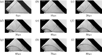
ns timing accuracy of the high-speed camera, was achieved by an output trigger signal sent from the pressure transducer, S1, to the high-speed camera. The signals from the pressure transducers were collected by a signal conditioner (PCB Piezotronics 482C), and recorded by a digital oscilloscope (LeCroy, Wave Surfer 24Xs-A). Figure 5 illustrates schlieren visualization with high temporal resolution, showing RR reflecting off the water with
 $M_{s}=1.52$
and
 $47^{\circ }$
deflection angle.
A series of schlieren photographs using a Phantom V711 camera showing shock reflection off a water surface at
 $M_{s}=1.52$
and
 $\unicode[STIX]{x1D703}_{w}=47^{\circ }$
resulting in regular reflection.

3.2.2 Schlieren visualization with high spatial resolution
Schlieren visualization with high spatial single-frame photographs were obtained using a digital-single lens reflex (DSLR) camera, a flash lamp (Nanolite KL-L Blitzlampe, High-speed Photo-system,
 $\pm 10$
ns timing accuracy) with an 18 ns duration and a flash lamp driver (high-speed photo-system). A Nikon D90 SLR camera was equipped with a 200 mm lens (AF Micro-Nikkor 200 mm
 $f$
/4 D IF-ED) to produce high spatial resolution images of
 $4288\times 2838$
pixels. The exposure time of the camera was set to 2.5 s, manually, in a dark room setting. The timing of the flash lamp was controlled by a delay generator (BNC Model 575,
 $\pm 0.8$
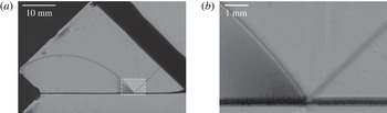
ns trigger accuracy) operated in single pulse shot mode with different delay times. The trigger signal was sent from pressure transducer S1 and collected by the signal conditioner. Figure 6 represents schlieren visualization with high spatial resolution. Figure 6(a,b) shows a regular reflection configuration over water.
Schlieren photographs using a Nikon D90 camera showing (a) regular reflection off a water surface for
 $M_{s}=1.38$
and
 $\unicode[STIX]{x1D703}_{w}=45^{\circ }$
and (b) a magnified image of the reflecting surface highlighted by the dashed rectangle in (a).

3.3 Experimental procedure
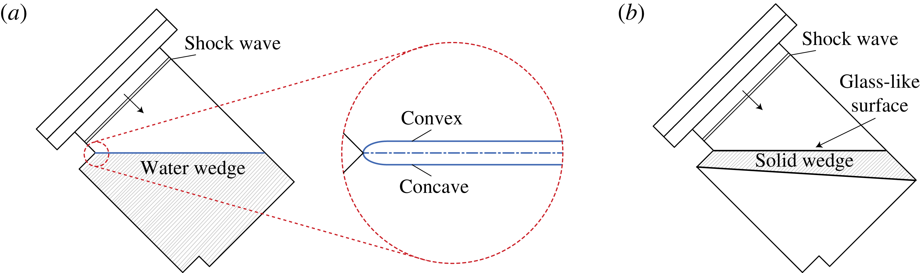
The water in the test section was changed every time in between experiments. A hydrophobic coating (Rain-X, SOPUS Products) was used on the windows of the test section to minimize the wetting condition and to clean the windows. There exists a small angle between the solid and the tangent line to the liquid surface, a contact angle, in the test section due to the liquid surface tension, as shown in figure 7(a). Since the purpose of this study was to find transition angles, it was necessary to observe whether a Mach stem is present above the liquid surface. If a concave meniscus occurs, the free surface cannot be visualized. As such, the curvature of the liquid was maintained to be slightly convex by filling the test section with liquid from the bottom (Takayama & Ben-Dor Reference Takayama and Ben-Dor1989). Figure 7(b) shows the side view of the test section with a solid wedge inserted.
Side view of the test section showing a schematic description: (a) a water wedge; (b) a solid wedge.

4 Results and analysis
The first set of simulations for each Mach number was initialized such that the reflection configuration was irregular. Therefore, a wedge angle of
 $25^{\circ }$
was chosen for the initial configuration. Then, the inclination angle was increased by steps of
 $1^{\circ }$
to determine at which angle the Mach stem and slipstream disappear and regular reflection occurs.
4.1 Validation of the experimental methodology
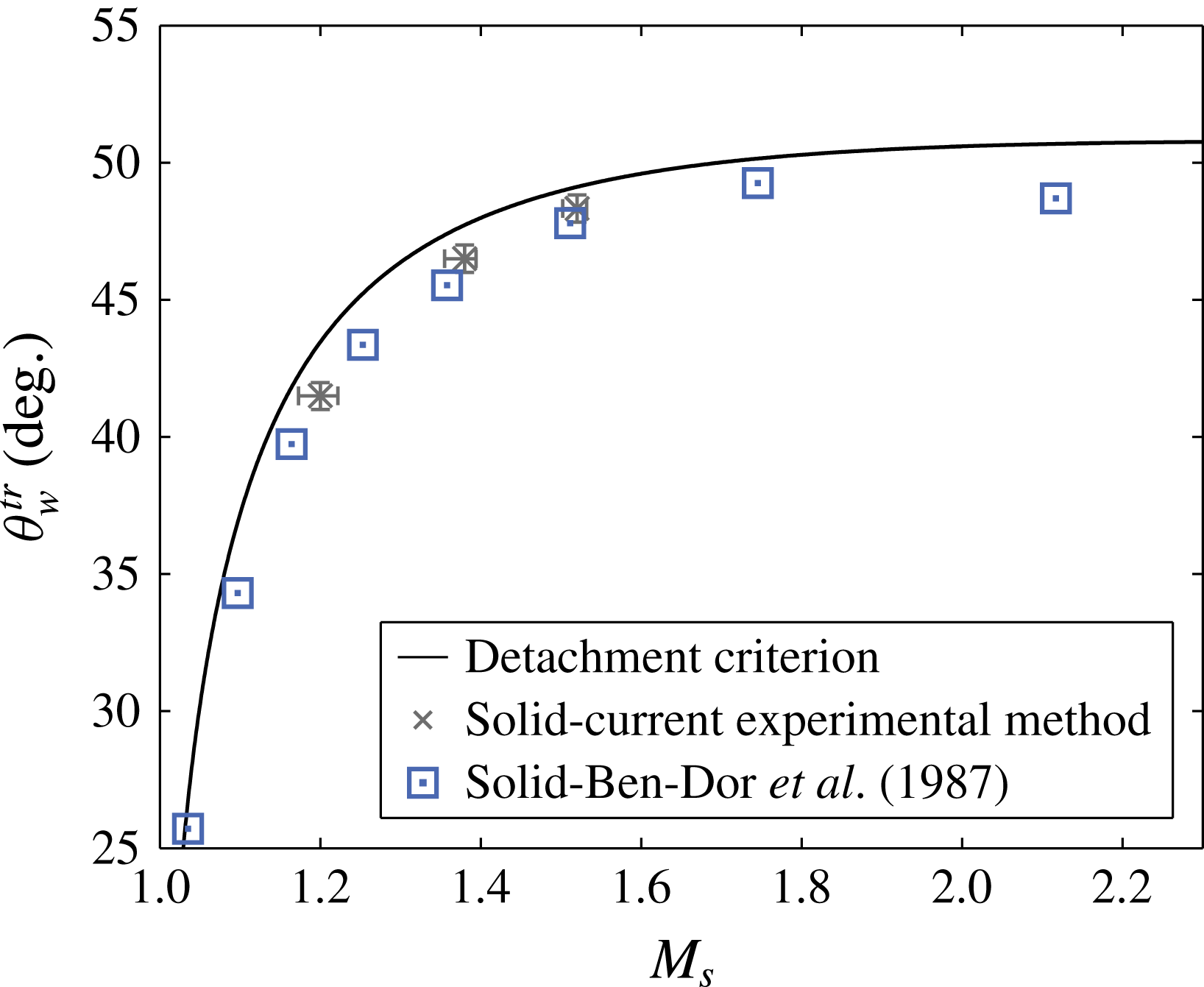
The experimental results obtained using the experimental method from the solid surface are validated against the previous experimental data. Figure 8 shows a comparison of the current experimental study and the previous experimental results (Ben-Dor et al. Reference Ben-Dor, Mazor, Takayama and Igra1987). A comparison to the previous data was made in terms of the transition angle for hydraulically smooth surface case. As it can be seen, a good agreement has been found for the transition angles. Therefore, based on the comparison between the previous and current results, the methodology in this study is able to ensure confidence in the accuracy for finding transition angles.
The transition angle measured by experimental method versus the incident shock Mach number compared to the previous results (Ben-Dor et al. Reference Ben-Dor, Mazor, Takayama and Igra1987). The size of the marker size represents the uncertainty of the previous study.

4.2 Comparison with experimental results
A direct comparison between schlieren visualizations obtained in the simulation and experiment with
 $M_{s}=1.38$
and
 $\unicode[STIX]{x1D703}_{w}=43^{\circ }$
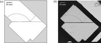
is shown in figure 9. Single-Mach reflection with a short Mach stem was observed in the simulation, while regular reflection was observed in the experiment. In the experiment, the thickness of the dark band representing the shock wave and the air–water interface that are obtained by using schlieren photography can be affected by several factors such as the strength of the shock wave, a non-parallel incident light angle and shadowgraph effects. Therefore, the dark band, especially, the air–water interface, looked thicker in the experiment than the simulation. If a Mach stem existed in these experiments, it could be covered by the air–water interface. However, the schlieren visualization for the simulation agrees well with regard to the incident and reflected shock wave locations of that for the experiment.
Comparison of schlieren visualizations for
 $M_{s}=1.38$
and
 $\unicode[STIX]{x1D703}_{w}=43^{\circ }$
for (a) simulation and (b) experiment.

4.3
 $RR\leftrightarrow IR$
transition angles

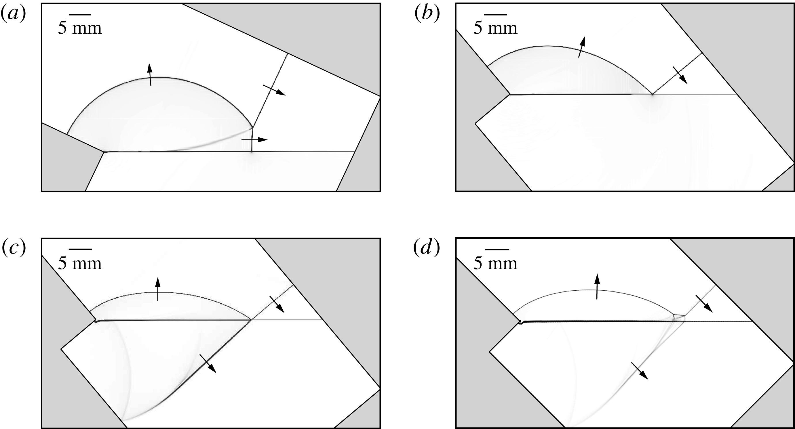
Schlieren images from simulations of different shock reflection configurations at different incident Mach numbers are shown in figure 10. Figure 10(a) shows the single-Mach reflection formed under Mach number
 $M_{s}=1.52$
and inclination wedge angle
 $\unicode[STIX]{x1D703}_{w}=25^{\circ }$
. Figure 10(b) shows the regular reflection formed using Mach number
 $M_{s}=1.52$
and wedge angle
 $\unicode[STIX]{x1D703}_{w}=50^{\circ }$
. Figure 10(c) shows the regular reflection formed under Mach number
 $M_{s}=4.0$
and wedge angle
 $\unicode[STIX]{x1D703}_{w}=50^{\circ }$
. The Mach number is much stronger than that used in figure 10(a,b). When the shock wave in air with Mach number
 $M_{s}=3$
or 4 impacts onto the water surface, the impact velocity is of the order of the speed of sound in water, and therefore a shock wave forms in the water and continues to propagate downstream, which is visualized in figure 10(c,d). Distortion of the water surface can be observed for strong incident shock cases (
 $M_{s}=3$
and 4). As shown in figure 10(c,d), the water surface near the wedge corner just started to deform, but the deformation is slow compared to the motion of shock wave. When the shock wave in air is weaker, the impact velocity is lower than the speed of sound in water, and thus no shock penetrates into the water region in the cases of figure 10(a,b). In previous experiments with shock wave reflection off water wedges done by Takayama & Ben-Dor (Reference Takayama and Ben-Dor1989), spherical shock waves that transmitted into a water medium were indeed observed for incident shock Mach numbers 2.33 and 2.30. For lower shock Mach numbers,
 $M_{s}=1.52$
, no spherical shock was observed. Figure 10(d) shows the more complex double-Mach reflection, with an incident Mach number
 $M_{s}=4.0$
and wedge angle
 $\unicode[STIX]{x1D703}_{w}=45^{\circ }$
.
Schlieren visualization showing types of different shock wave reflection configurations off a water wedge. (a) Single-Mach reflection for
 $M_{s}=1.52$
and
 $\unicode[STIX]{x1D703}_{w}=25^{\circ }$
. (b) Regular reflection for
 $M_{s}=1.52$
and
 $\unicode[STIX]{x1D703}_{w}=50^{\circ }$
. (c) Regular reflection for
 $M_{s}=4.0$
and
 $\unicode[STIX]{x1D703}_{w}=50^{\circ }$
. (d) Double-Mach reflection for
 $M_{s}=4.0$
and
 $\unicode[STIX]{x1D703}_{w}=45^{\circ }$
.

Single-Mach reflection was observed for lower Mach numbers,
 $M_{s}=1.20$
, 1.38, 1.52 and 2, while double-Mach reflection was observed for higher Mach numbers,
 $M_{s}=3$
and 4. In cases of single-Mach reflection, a Mach stem was generated right after the incident shock reached the water wedge, and the length of the Mach stem kept growing as the incident shock wave travelled further downstream. Simultaneously, a slipstream formed behind the Mach stem.
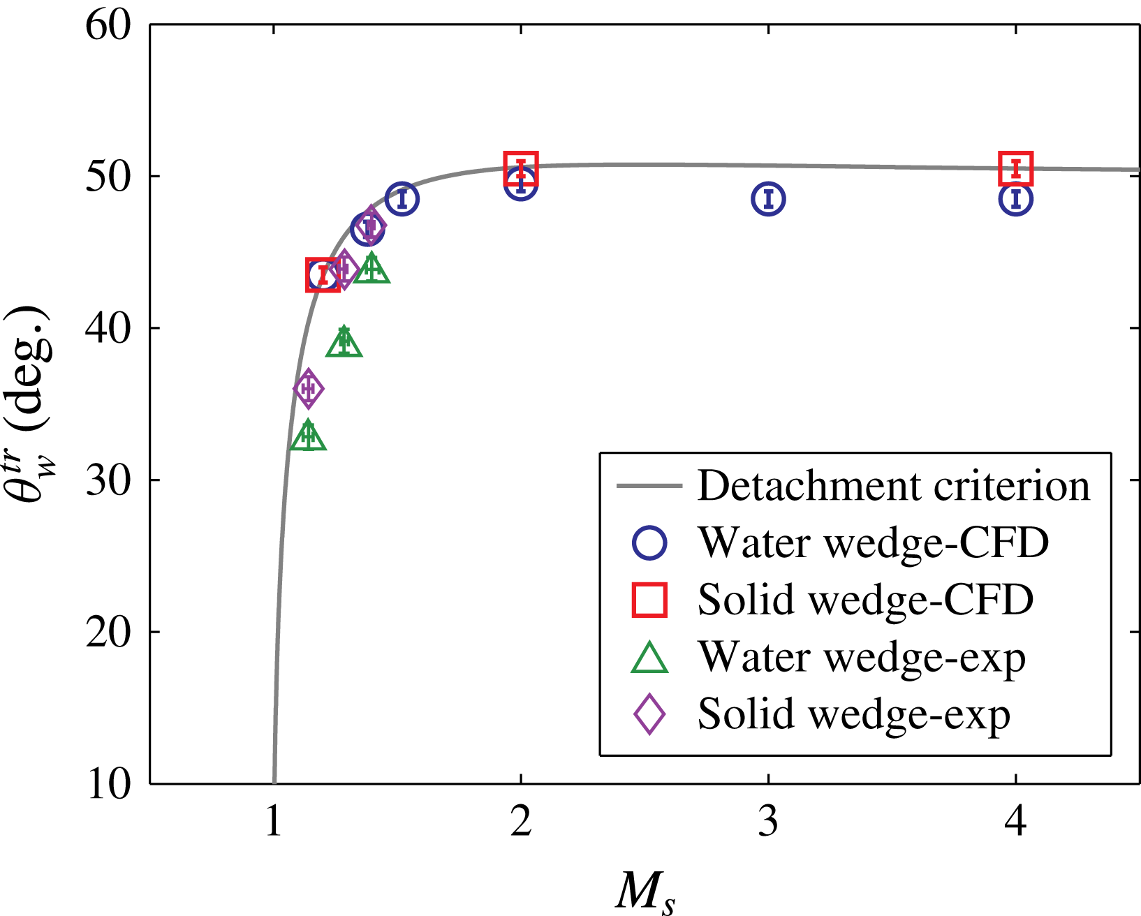
Figure 11 shows a comparison of the detachment criterion and transition angles for the water and solid wedge cases obtained from the simulations and the experiments. The difference between transition angles obtained from the simulations and those predicted by the detachment criterion is less than 5.3 %.
Transition angles for water and solid wedge cases observed from simulations and experiments for different incident shock Mach numbers. Detachment criterion (Mouton Reference Mouton2006) plotted for comparison. In the simulation, the transition angles for water wedge cases are measured for six different shock Mach numbers
 $M_{s}=1.20$
, 1.38, 1.52, 2, 3 and 4, while it is measured only for three Mach numbers
 $M_{s}=1.20$
, 2 and 4 for the case of a solid wedge. In the experiment, three different shock Mach numbers,
 $M_{s}=1.20$
, 1.38 and 1.52, are measured.

In the simulation, the transition angles for solid wedge cases agreed with the detachment criterion. However, in the experiment, the transition angles for solid wedge were measured
 $1.5^{\circ }$
lower than the detachment criterion. This is not surprising, since both the simulations of solid wedge cases and the detachment criterion assume inviscid flow and rigid smooth wedge surface and the viscous effects delay the transition from the regular reflection to the Mach reflection (Kleine et al.
Reference Kleine, Timofeev, Hakkaki-Fard and Sadot2014). The difference between the results of the water wedge cases and the detachment criterion is within
 $2.7^{\circ }$
in the simulation and
 $4.5^{\circ }$
in the experiment, which may result from the fact that part of the shock energy was absorbed by water during the reflection. The difference between the simulation and the experiments was mainly caused by the deficiency of viscous effect in the simulation and the thicker air–water interface in the experiment. Another error source for the water wedge cases comes from the use of a multicomponent treatment of the volume fractions in the governing equations, see § 2. In addition, some artificial mixing of air and water will invariably occur in cells crossed by the two-fluid interface. While the influence of this effect on the overall solution is mitigated by our use of local mesh refinement, an ad hoc treatment of the boundary between the two immiscible fluids is unavoidable. Also note that water surface tension is currently not considered in the simulations.
4.4 Comparison between water and solid wedge cases
A direct comparison of transition angles for the water and solid wedge cases for Mach numbers
 $M_{s}=1.20$
, 2 and 4 is shown in figure 11. For Mach number
 $M_{s}=1.20$
, the transition angles of water and solid wedge cases are in the same range
 $43^{\circ }<\unicode[STIX]{x1D703}_{w}<44^{\circ }$
. For Mach numbers
 $M_{s}=2$
and 4, the transition angles are in the range
 $50^{\circ }<\unicode[STIX]{x1D703}_{w}<51^{\circ }$
for solid wedge cases, which fit well for the theoretical solution; while the transition angles are in the range
 $49^{\circ }<\unicode[STIX]{x1D703}_{w}<50^{\circ }$
and
 $48^{\circ }<\unicode[STIX]{x1D703}_{w}<49^{\circ }$
respectively for water wedge cases, which are
 $0.5^{\circ }{-}1.6^{\circ }$
lower than the theoretical solution.
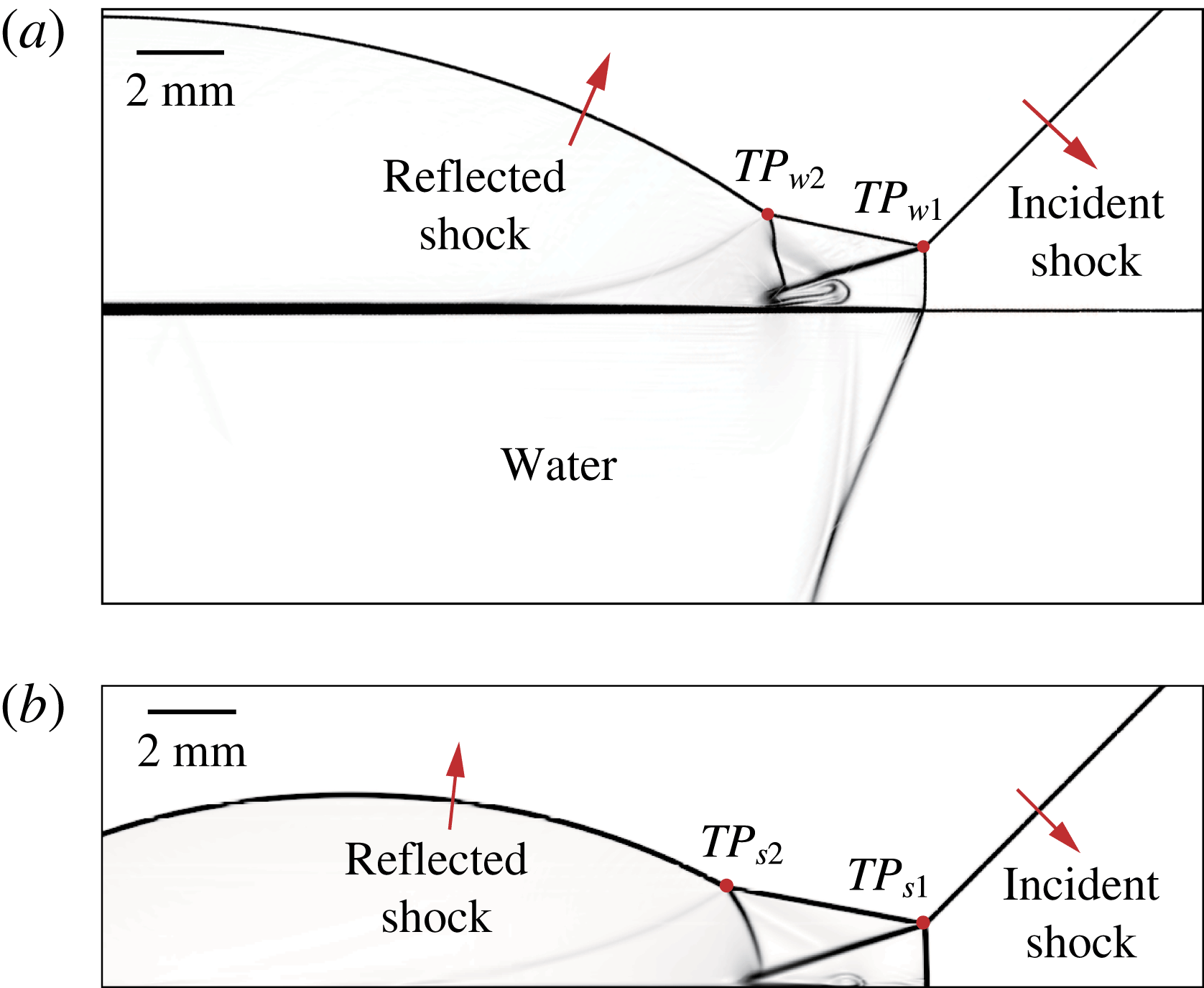
Schlieren images for the water and solid wedge cases under the same conditions,
 $M_{s}=3$
and
 $\unicode[STIX]{x1D703}_{w}=45^{\circ }$
, are shown in figure 12, where (a) shows the reflection off the water wedge at time instant
 $t=31.5~\unicode[STIX]{x03BC}\text{s}$
, and (b) shows the reflection off the solid wedge at time instant
 $t=23.5~\unicode[STIX]{x03BC}\text{s}$
. Specifically, the Mach stems of the above two cases are of the same length. Comparing figure 12(a) with 12(b) it is clear that under this condition the reflection is double-Mach type for both cases. The first and second triple points were denoted as
 $TP_{w1}$
and
 $TP_{w2}$
in the water wedge cases, and
 $TP_{s1}$
and
 $TP_{s2}$
in the solid wedge cases. The two reflection configurations above the reflecting surface have similar shape, but the distance between the two triple points are longer in the solid wedge case. The quantification of the reflection structure can be realized by measurement of the triple point trajectories, and corresponding analysis will be further discussed in § 4.5.
Schlieren visualization of shock wave reflection off (a) a water wedge at time instant
 $t=31.5~\unicode[STIX]{x03BC}\text{s}$
and (b) a solid wedge at time instant
 $t=23.5~\unicode[STIX]{x03BC}\text{s}$
, with
 $M_{s}=3$
and
 $\unicode[STIX]{x1D703}_{w}=45^{\circ }$
. The Mach stems in (a,b) are of the same length.

4.5 Triple point trajectory
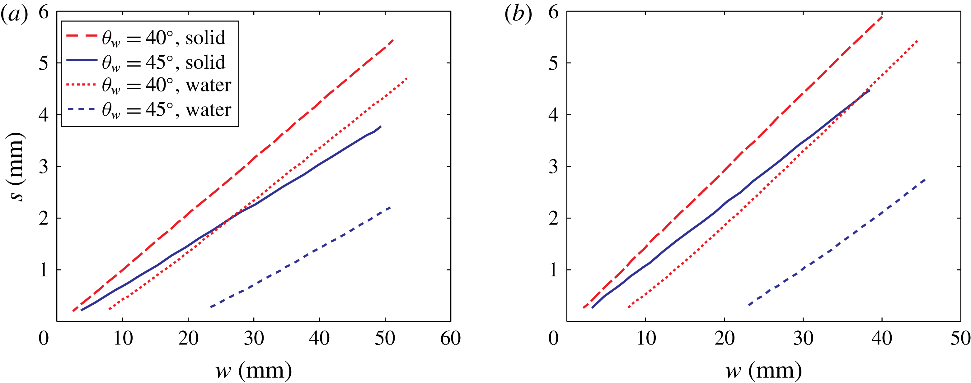
Setting the compressive corner as the origin, the displacement of the first and second triple points in the horizontal (
 $w$
) and the vertical (
 $s$
) directions with incident shock Mach number
 $M_{s}=4$
is plotted in figure 13. Two different inclination angles (
 $\unicode[STIX]{x1D703}_{w}=40^{\circ }$
and
 $45^{\circ }$
) were considered for both solid and water wedge cases. As shown in figure 13, the triple point trajectories are straight lines, which corresponds to a linear growth of the Mach stem, as previously reported by Hornung & Robinson (Reference Hornung and Robinson1982). Figure 13 also shows that
 $s$
grows faster for lower inclination angles.
The (a) first and (b) second triple point trajectories with Mach number
 $M_{s}=4$
and two different inclination angles for solid and water wedge cases.

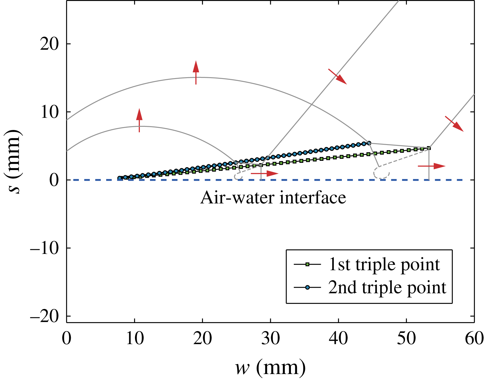
Figure 14 shows both the first and second triple point trajectories for shock reflection off water wedge with
 $M_{s}=4$
and
 $\unicode[STIX]{x1D703}_{w}=40^{\circ }$
. At each time instant, the height of the second triple point was always larger than the first triple point.
The first and second triple point trajectories for shock wave reflection off a water wedge with Mach number
 $M_{s}=4$
and inclination angle
 $\unicode[STIX]{x1D703}_{w}=40^{\circ }$
.

In the case of double-Mach reflection over the water wedge, both the first and second triple points appeared and started to rise off the surface later than in the cases of the solid wedge with the same
 $M_{s}$
and
 $\unicode[STIX]{x1D703}_{w}$
. This delay increased for higher values of
 $\unicode[STIX]{x1D703}_{w}$
. One likely reason is that, in the solid wedge cases, no deformation of the surface occurred, where all the energy was reflected at the solid surface during the impact and sustained the growth of the reflection above the solid surface. However, in the water wedge cases, although the air–water interface did not have time to deform in the simulation, part of the energy was absorbed by water during the impact, which reduced the energy reflected from the air–water interface, leading to a reduction of the available energy used to support the growth of the Mach stem. Also, vortices were observed near the water surface behind the Mach stem, shown in figure 12(a), which also consumed some of the energy. The vortices are not artefacts, but are due to the rotational flow. In figure 12, the flow behind the Mach stems are subsonic, and cannot cross the slipstream. In the reference frame of the first triple point, the velocity of the flow near the slipstream is parallel to the slipstream. When the flow reaches the water surface or the solid wedge surface, the flow velocity is forced to be altered to the direction that is parallel to the wedge surface, so rotational flow forms at the foot of the slipstream. As
 $\unicode[STIX]{x1D703}_{w}$
was increased while keeping
 $M_{s}$
as constant, the vertical component of the incident shock Mach number increased, which resulted in an increase in the energy transmitted into the water region. Due to the decrease of energy for supporting Mach stem growth, this delay increased as
 $\unicode[STIX]{x1D703}_{w}$
was increased. Though the establishment of the Mach stem is delayed for the water wedge cases, the growth of the reflection configuration is linear, which can be seen in figures 13 and 14, and therefore the shock reflection process can be described as self-similar.
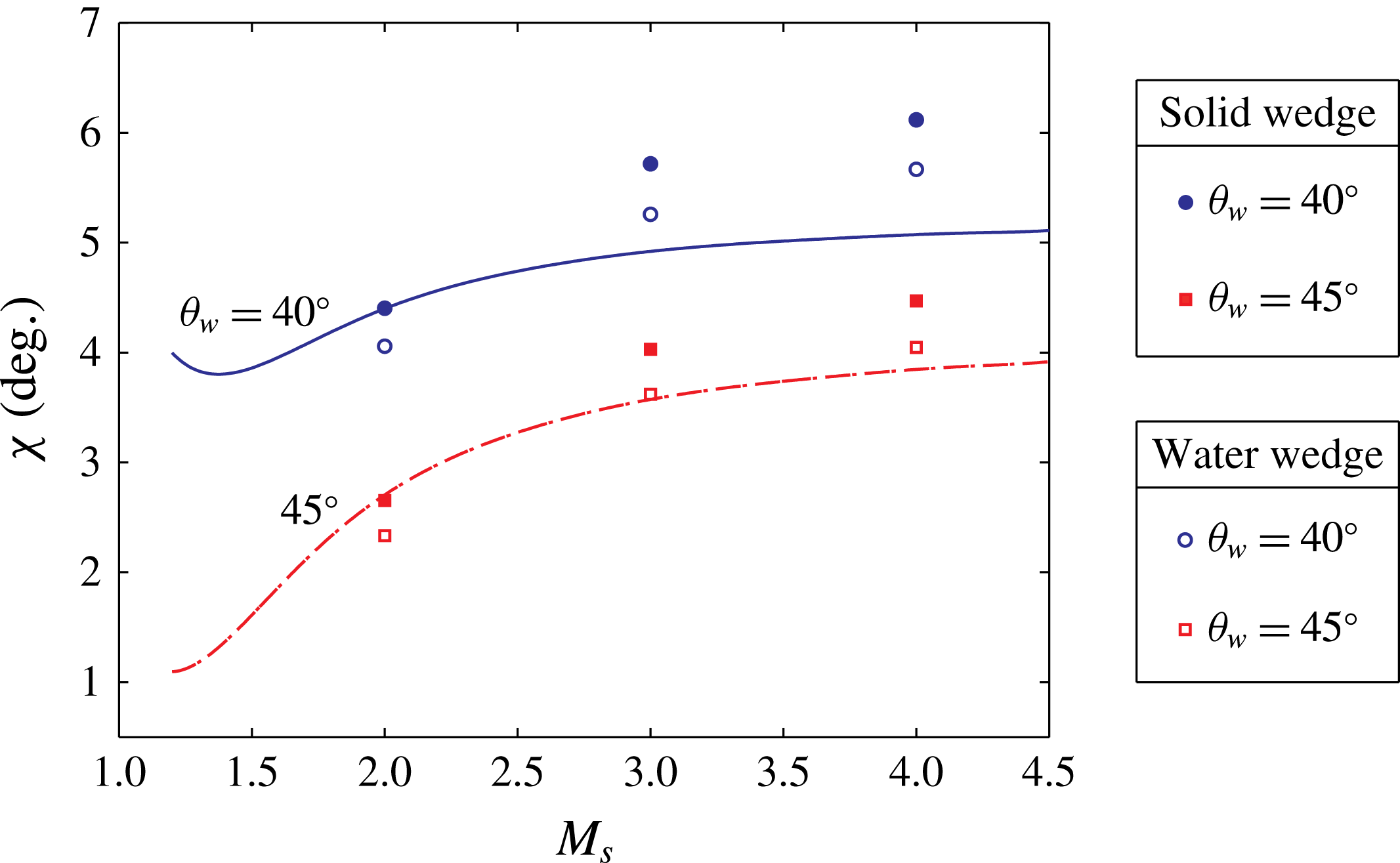
The triple point trajectory angle was calculated based on linear curve fitting of the trajectory. Figure 15 shows the measurement of the first triple point trajectory angle,
 $\unicode[STIX]{x1D712}$
, from the simulations. The analytic solution from Ben-Dor (Reference Ben-Dor1978) is plotted for comparison. For the solid wedge cases, the difference between the measurement and analytic solution is within
 $1.1^{\circ }$
. For the water wedge cases, the difference is less than
 $0.6^{\circ }$
. One likely reason for the difference between solid and water wedge cases is that energy is transmitted into the liquid but not to the solid.
The first triple point trajectory angle,
 $\unicode[STIX]{x1D712}$
, for water and solid wedge cases obtained from simulations with different
 $M_{s}$
and
 $\unicode[STIX]{x1D703}_{w}$
. Analytic solutions from Ben-Dor (Reference Ben-Dor1978) are plotted for comparison.

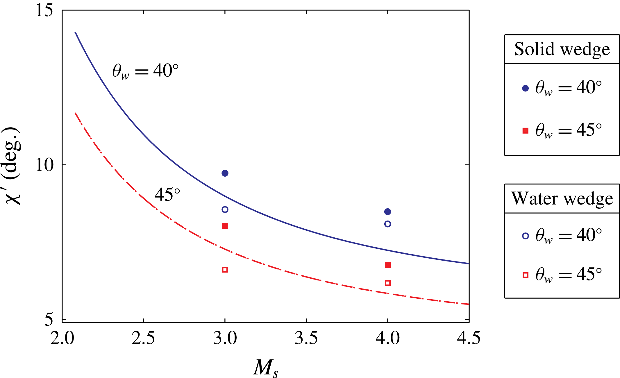
The second triple point trajectory angle,
 $\unicode[STIX]{x1D712}^{\prime }$
, for water and solid wedge cases obtained from simulations with different
 $M_{s}$
and
 $\unicode[STIX]{x1D703}_{w}$
. Analytic solutions from Ben-Dor (Reference Ben-Dor1980) are plotted for comparison.

Figure 16 shows the measurement of the second triple point trajectory angle,
 $\unicode[STIX]{x1D712}^{\prime }$
, compared with the analytic solution from Ben-Dor (Reference Ben-Dor1980). For the solid wedge cases, the agreement is within
 $1.3^{\circ }$
. For the water wedge cases, the difference is less than
 $0.9^{\circ }$
. One possible reason for the deviation is that the analytic solution assumed uniform flow behind reflected shock wave and Mach stems, while this assumption is not true in the simulated cases.
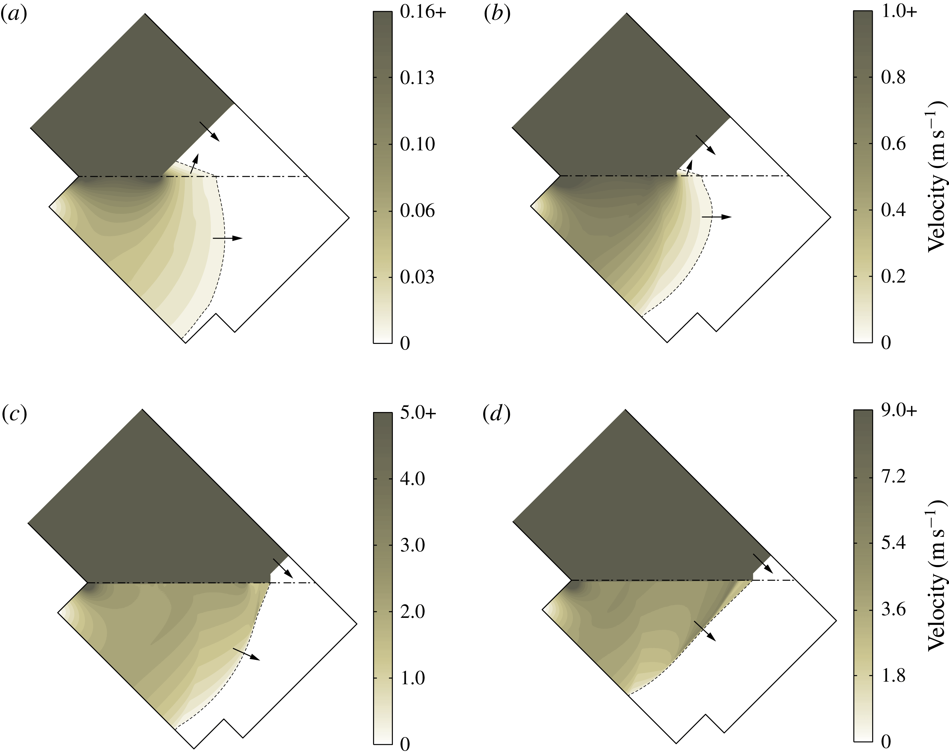
Velocity profile inside water under the incident shock Mach numbers (a)
 $M_{s}=1.2$
, (b)
 $M_{s}=2$
, (c)
 $M_{s}=3$
and (d)
 $M_{s}=4$
, and wedge angle
 $\unicode[STIX]{x1D703}_{w}=45^{\circ }$
.

4.6 Transmitted waves in water
Figure 17 shows the velocity profile of the transmitted waves in the water under four different incident shock Mach numbers from the simulation. The threshold of the visualized velocity is chosen so that more details of the flow features inside water can be captured, while the flow behind the incident shock wave and Mach stem in the air are not visualized. As shown in figure 17(a,b), the velocity change across the compression wave is smooth, thus the transmitted waves in the water are not shock waves. In particular, in the case of figure 17(a), which shows a regular reflection, the incident shock wave is striking the water surface at an angle of
 $45^{\circ }$
. The foot of the incident shock wave is sliding over the water surface with a uniform speed
 $v_{i}=587~\text{m}~\text{s}^{-1}$
. Through calculation, the speed of the compression wave in the water is approximately
 $v_{t}\approx 1122~\text{m}~\text{s}^{-1}$
, which is lower than the speed of sound in water (
 $1452~\text{m}~\text{s}^{-1}$
). In the case of figure 17(b), illustrating a single-Mach reflection, the foot of the Mach stem is traversing at the speed
 $v_{i}=1023~\text{m}~\text{s}^{-1}$
, while the speed of the compression wave in the water is
 $v_{t}\approx 1249~\text{m}~\text{s}^{-1}$
. In the above two cases, the transmitted waves in the water are weak, thus no shock wave is formed in the water. Also, the foot of the incident shock wave or Mach stem cannot catch up with the corner-generated signal travelling in the water, so a precursor wave is induced ahead of the Mach stem that passes the information from water back into the air, as previously reported by Rodriguez et al. (Reference Rodriguez, Jourdan, Marty, Allou and Parisse2016). In figure 17(c,d), different from (a) and (b), the precursor wave no longer appears. The Mach stems in (c) and (d) are moving with uniform speeds
 $v_{i}=1575~\text{m}~\text{s}^{-1}$
and
 $2109~\text{m}~\text{s}^{-1}$
respectively, which are larger than the speed of sound in water. Thus, a shock wave is formed in the water due to the superposition of the compression waves, and the shock is attached to the Mach stem at every instant.
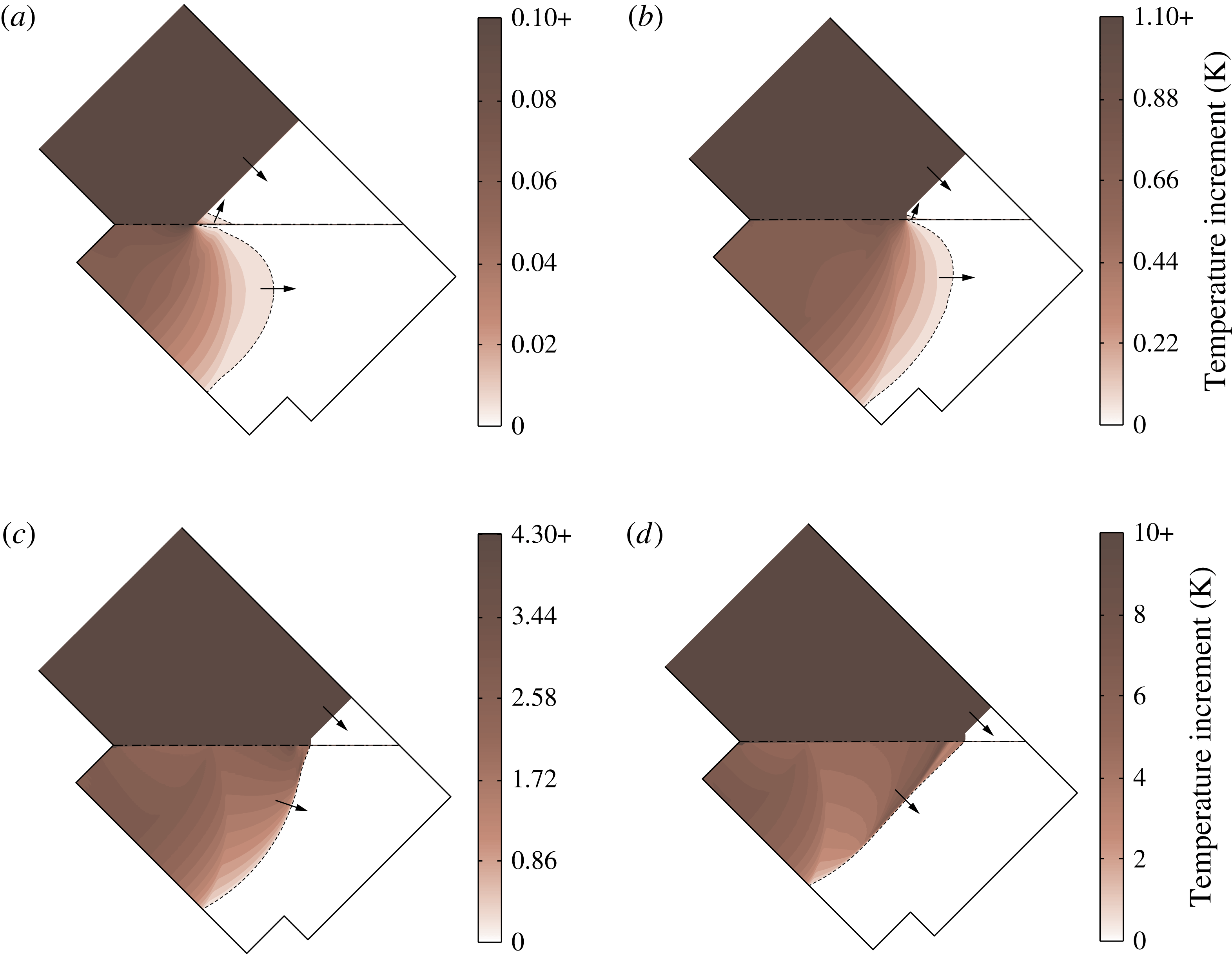
Temperature increment in the water for incident shock Mach numbers (a)
 $M_{s}=1.2$
, (b)
 $M_{s}=2$
, (c)
 $M_{s}=3$
and (d)
 $M_{s}=4$
, and wedge angle
 $\unicode[STIX]{x1D703}_{w}=45^{\circ }$
.

4.7 Temperature change in water
Figure 18 shows the temperature increments in the water for four different incident shock Mach numbers from the simulation. The temperature increment is chosen to be plotted in a certain range so that the changes in the water is clearly visualized, while the temperature field behind the incident shock wave and Mach stem above the air–water interface are not visualized. As shown in figure 18(a,b), though the corner-generated signal propagates fast inside the water, the temperature increment in the water is less than 1 K. In particular, the temperature change for the
 $M_{s}=1.2$
case is less than 0.1 K. However, in the cases of figure 18(c,d), a shock wave forms in the water, and a temperature discontinuity is observed across the shock wave. The temperature increment across the shock front in the water is approximately 3.0 K and 7.3 K respectively in figures 18(c) and 18(d).
5 Conclusions
In this work, a comprehensive numerical study of shock wave reflection off water wedge was done, supported by experimental results. Different shock wave reflection patterns, transition angles and triple point trajectory angles were studied and compared with reflection off solid wedges.
The major contributions can be summarized as follows. First, high resolution numerical simulations and experiments are performed to study shock wave reflections off water surface. The wave patterns are comprehensively investigated in terms of transition angles and triple point trajectories. Also, simulations are compared against both experimental results and theoretical solutions for the solid wedge cases. The difference between the solid and water wedge cases is analysed and physically explained. Furthermore, the transmitted waves inside the water are quantitatively studied with regard to the velocity profile and the temperature field. Results from the low and high incident shock Mach numbers are compared and two different scenarios are found.
In particular, planar shock wave reflections over water and solid wedges were numerically explored using six different shock Mach numbers,
 $M_{s}=1.2$
, 1.38, 1.52, 2, 3 and 4, and experimentally investigated using three different shock Mach numbers,
 $M_{s}=1.20$
, 1.38 and 1.52. For both solid and water wedge cases, transition angles show agreement within 5.3 % measured from simulations and 9.2 % measured from experiments comparing with the theoretical detachment criterion for a solid surface.
Moreover, comparing results of the water with solid wedge cases, the transition angle is the same for shock Mach number
 $M_{s}=1.20$
, while the difference gets larger as Mach number increases. Though the establishment of the Mach stem is earlier, the reflection configuration of the solid wedge case has a similar shape as the water wedge case. The difference in wave pattern is primarily due to the energy transmission into the water wedge, which does not exist in the solid wedge case.
The triple point locations for both water and solid wedge cases were traced in the simulation. Results showed that the triple point trajectories are linear. The first and second triple point trajectory angles,
 $\unicode[STIX]{x1D712}$
and
 $\unicode[STIX]{x1D712}^{\prime }$
, were measured and compared with the analytic solution. Close agreement, within
 $1.3^{\circ }$
and
 $0.9^{\circ }$
respectively, was found for the solid and water wedge cases.
The transmitted waves inside the water under four different Mach numbers from the simulations were visualized. Results showed that under relatively low incident shock Mach numbers,
 $M_{s}=1.2$
and 2, a precursor wave is induced that passes information from water back into the air. At relatively high Mach numbers,
 $M_{s}=3$
and 4, there is no precursor wave, but a shock wave is formed inside the water and it is attached to the Mach stem at every instant.
The temperature field in the water is visualized. For low incident shock Mach numbers,
 $M_{s}=1.2$
and 2, the temperature increment in the water is less than 1 K. For the two higher incident shock Mach numbers,
 $M_{s}=3$
and 4, the temperature difference across the shock wave in the water is approximately 3.0 K and 7.3 K, respectively.
The numerical result for the case of incident shock Mach number
 $M_{s}=1.20$
and inclination wedge angle
 $\unicode[STIX]{x1D703}_{w}=40^{\circ }$
was compared with the experimental data using schlieren visualization. Results showed good agreement in terms of shock wave configuration.
Acknowledgements
The authors wish to thank the High Performance Computing Center at University of Southern California for providing free access to computing resources. This study is supported by the National Science Foundation under grant no. CBET-1437412.